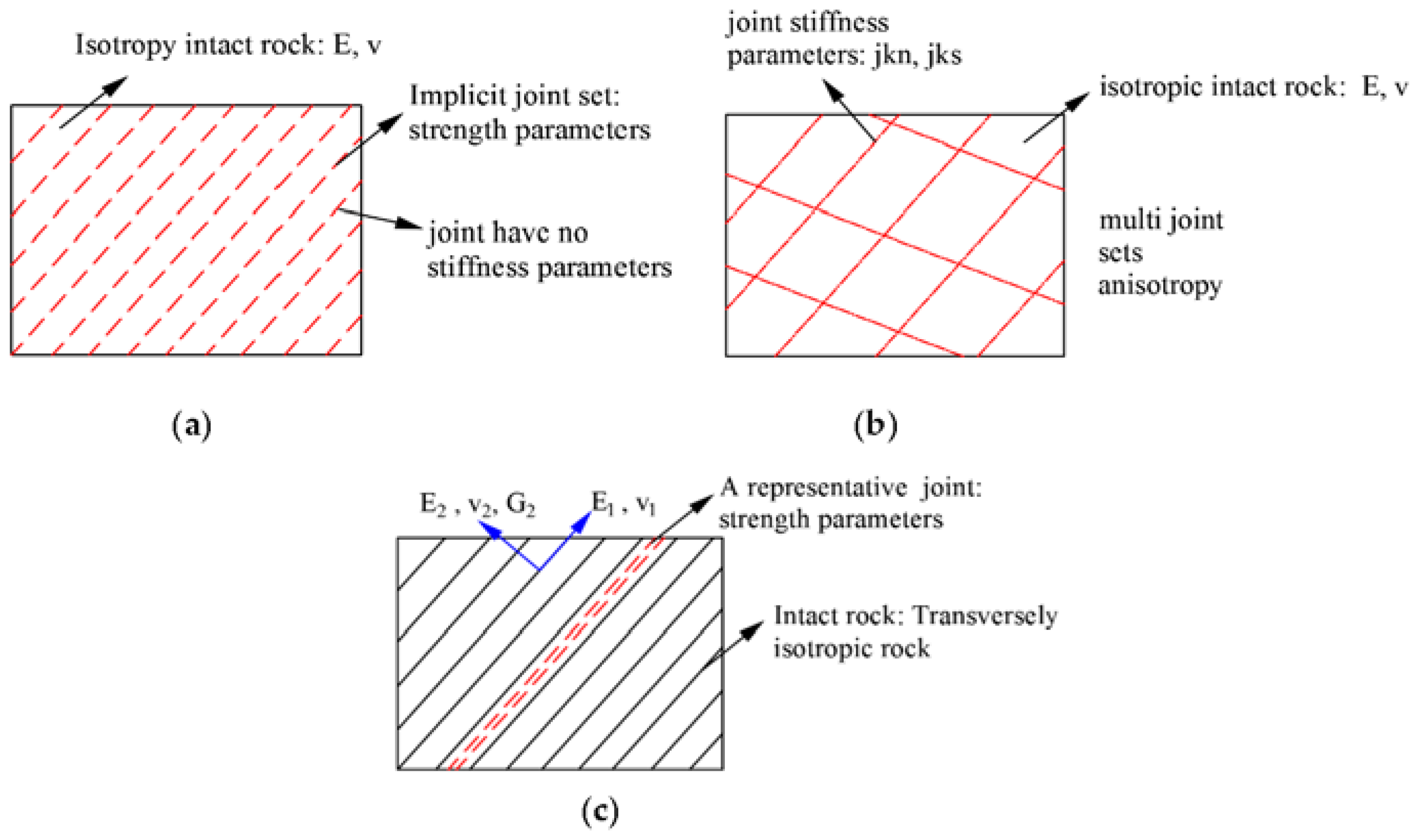
Figure 1.
Schematic for isotropic and anisotropic models: (a) ubiquitous joint model, (b) multi joint model, (c) anisotropic model with transversely isotropic rock matrix and representative joint orientation.
Figure 1.
Schematic for isotropic and anisotropic models: (a) ubiquitous joint model, (b) multi joint model, (c) anisotropic model with transversely isotropic rock matrix and representative joint orientation.
Figure 2.
Jointed rock mass containing three random joint sets.
Figure 2.
Jointed rock mass containing three random joint sets.
Figure 3.
Downgraded stiffness for the equivalent continua.
Figure 3.
Downgraded stiffness for the equivalent continua.
Figure 4.
Determination of active surfaces and definition the multi-surface regions.
Figure 4.
Determination of active surfaces and definition the multi-surface regions.
Figure 5.
Mohr-Coulomb failure criterion with tension cut-off for matrix and joint.
Figure 5.
Mohr-Coulomb failure criterion with tension cut-off for matrix and joint.
Figure 6.
Failure criterion for intact rock and joint set in combination with different stress states: (a) Position B and C, (b) Position D and E, (c) Position F and G, (d) illustration of corresponding orientations of weak planes.
Figure 6.
Failure criterion for intact rock and joint set in combination with different stress states: (a) Position B and C, (b) Position D and E, (c) Position F and G, (d) illustration of corresponding orientations of weak planes.
Figure 7.
Schematic illustration for rock mass strength anisotropy: (a) Jaeger’s curve, (b) dominant failure area for weak plane and for rock matrix.
Figure 7.
Schematic illustration for rock mass strength anisotropy: (a) Jaeger’s curve, (b) dominant failure area for weak plane and for rock matrix.
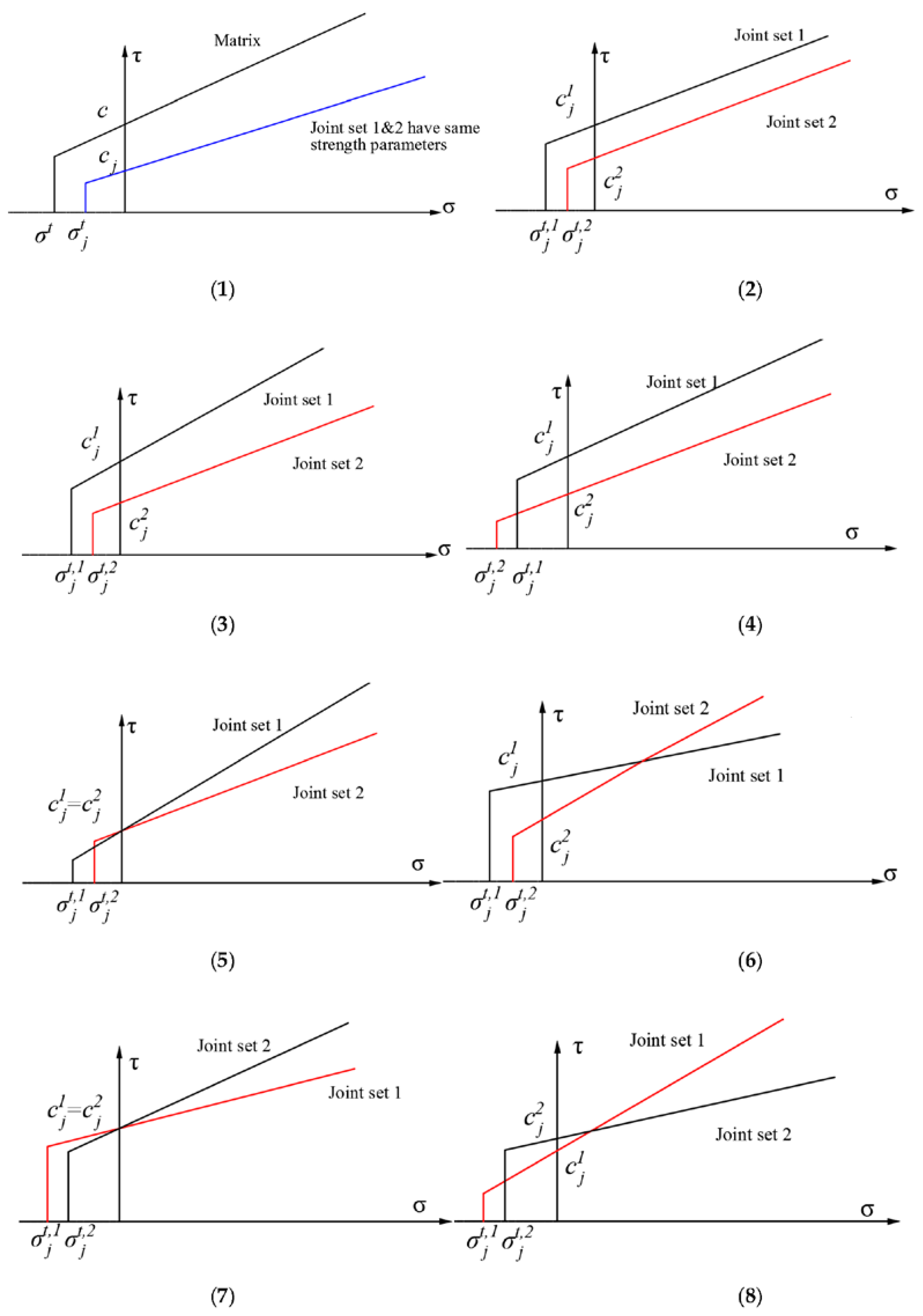
Figure 8.
Sketch of potential failure envelops for two joints sets corresponding to the constellations 1–8 in
Table 1.
Figure 8.
Sketch of potential failure envelops for two joints sets corresponding to the constellations 1–8 in
Table 1.
Figure 9.
Failure areas for weak planes and rock matrix. (a) Increasing vertical stress reached a critical state for joint set 2; (b) Critical state for rock matrix and failure areas for weak planes; (c) Failure areas for weak planes and for rock matrix.
Figure 9.
Failure areas for weak planes and rock matrix. (a) Increasing vertical stress reached a critical state for joint set 2; (b) Critical state for rock matrix and failure areas for weak planes; (c) Failure areas for weak planes and for rock matrix.
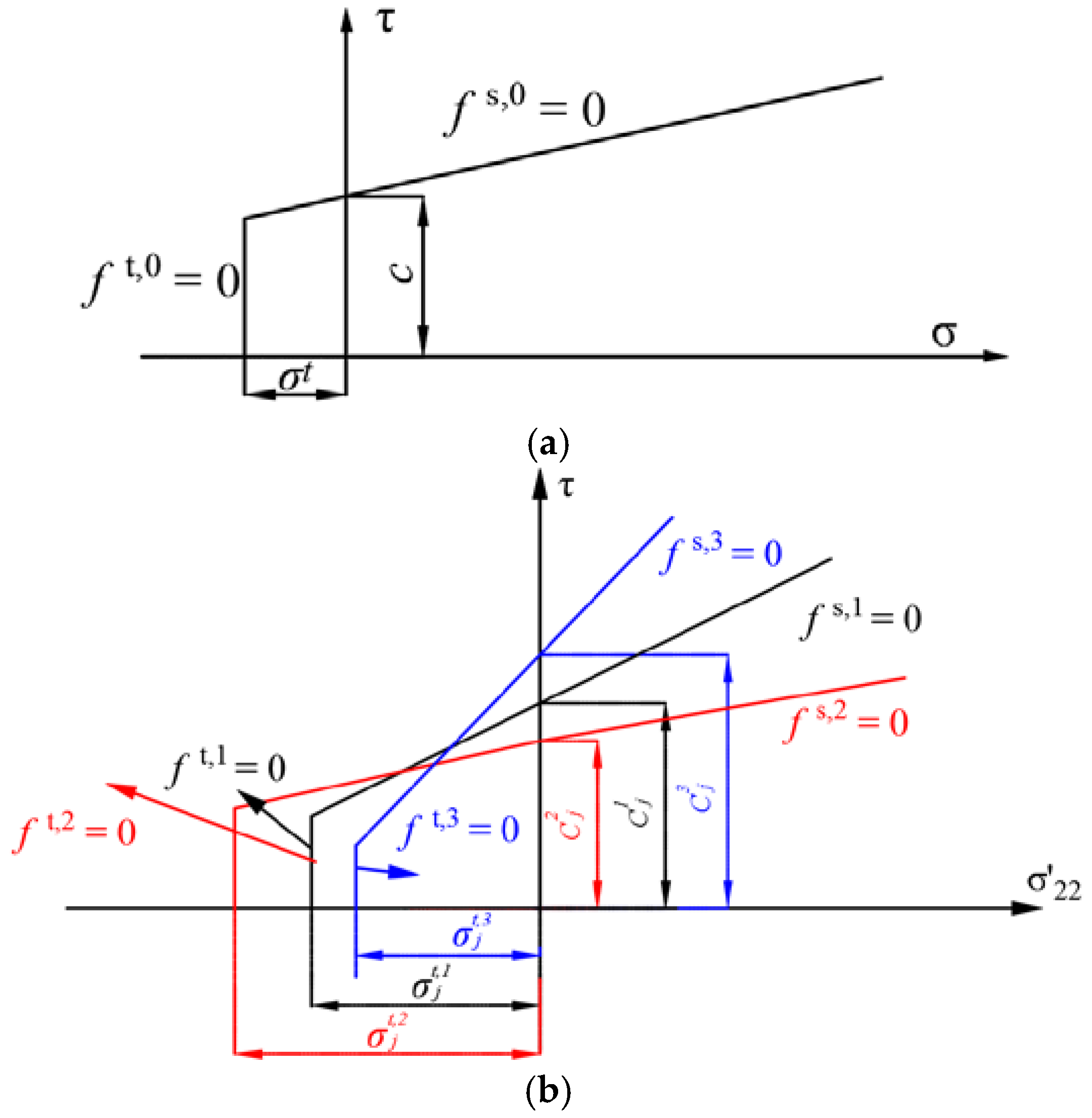
Figure 10.
Two kinds of joint failure criteria for a jointed rock mass. (
a) Joint failure criterion for constellations 1–4 (see
Table 1); (
b) Multi-stage failure criteria for joints having different parameters; (
c) Eight sections for solving the multi-surface plasticity problem.
Figure 10.
Two kinds of joint failure criteria for a jointed rock mass. (
a) Joint failure criterion for constellations 1–4 (see
Table 1); (
b) Multi-stage failure criteria for joints having different parameters; (
c) Eight sections for solving the multi-surface plasticity problem.
Figure 11.
(a) Illustration of the intact rock failure criterion; (b) Three joint failure criteria in a multi-joint model.
Figure 11.
(a) Illustration of the intact rock failure criterion; (b) Three joint failure criteria in a multi-joint model.
Figure 12.
Flowchart for equivalent continuum multi-joint model.
Figure 12.
Flowchart for equivalent continuum multi-joint model.
Figure 13.
Mohr’s circle and stress state on failure plane.
Figure 13.
Mohr’s circle and stress state on failure plane.
Figure 14.
(
a) Failure envelop for sample with two perpendicular joints under uniaxial compression (see
Table 2); (
b) Schematic of 5 sample with two perpendicular joints (A to E).
Figure 14.
(
a) Failure envelop for sample with two perpendicular joints under uniaxial compression (see
Table 2); (
b) Schematic of 5 sample with two perpendicular joints (A to E).
Figure 15.
Failure envelope for sample with different friction values (see
Table 3).
Figure 15.
Failure envelope for sample with different friction values (see
Table 3).
Figure 16.
Failure envelope for sample with different joint cohesion values (see
Table 4).
Figure 16.
Failure envelope for sample with different joint cohesion values (see
Table 4).
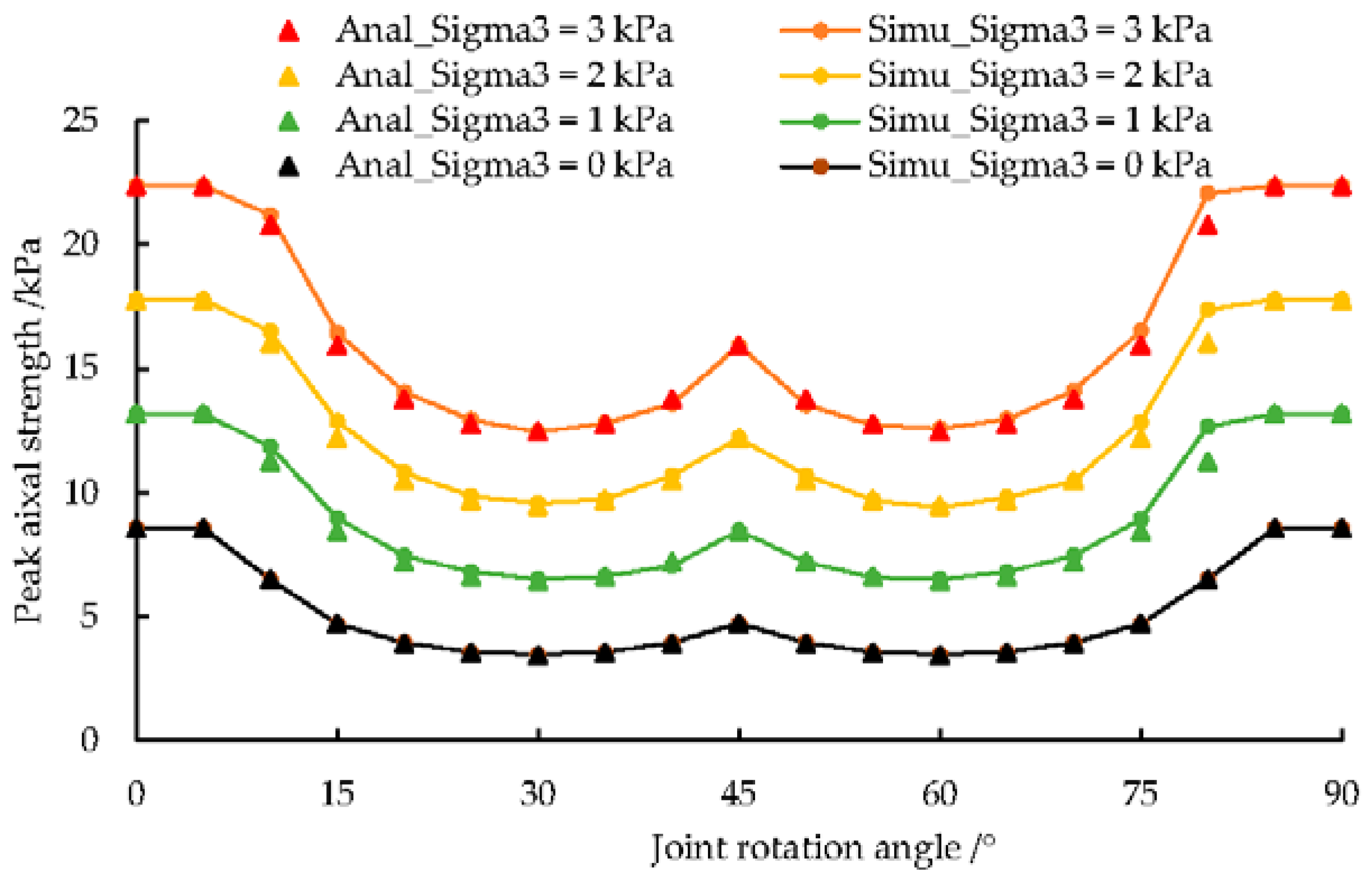
Figure 17.
Peak strength versus orientation of joint system under various confining pressures.
Figure 17.
Peak strength versus orientation of joint system under various confining pressures.
Figure 18.
(a) Schematic diagram for samples with three joints; (b) UCS for sample with three joints: multi-joint model (line) and analytical solution (triangular) versus joint set angle.
Figure 18.
(a) Schematic diagram for samples with three joints; (b) UCS for sample with three joints: multi-joint model (line) and analytical solution (triangular) versus joint set angle.
Figure 19.
Sketch of model geometry and boundary conditions.
Figure 19.
Sketch of model geometry and boundary conditions.
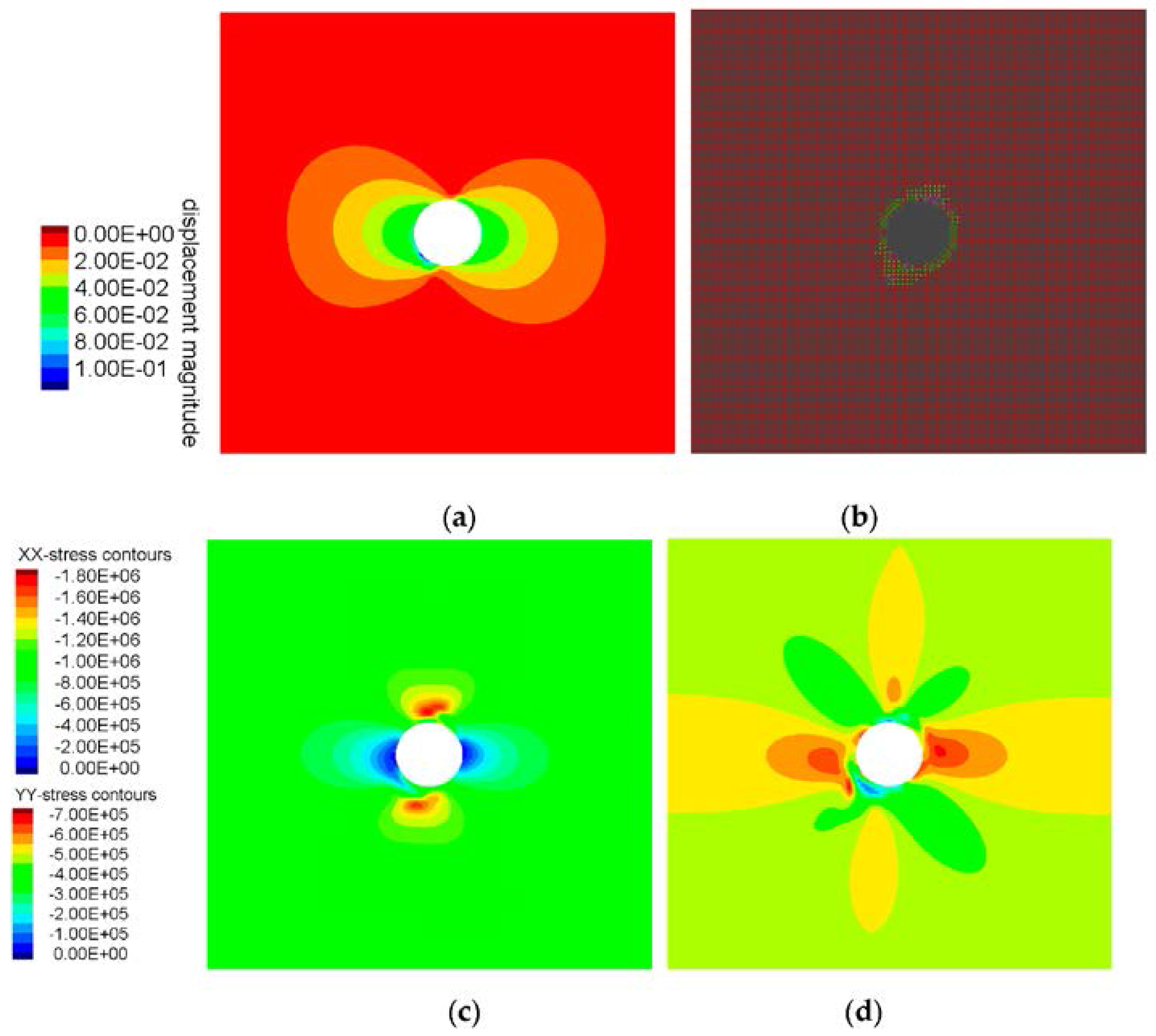
Figure 20.
Simulation results for tunnel model with joint orientation of −60° and κ = 1: (a) displacement contours [m], (b) plasticity state, (c) contour plot of horizontal stresses [Pa] and (d) contour plot of vertical stresses [Pa].
Figure 20.
Simulation results for tunnel model with joint orientation of −60° and κ = 1: (a) displacement contours [m], (b) plasticity state, (c) contour plot of horizontal stresses [Pa] and (d) contour plot of vertical stresses [Pa].
Figure 21.
Simulation results for tunnel model with joint orientation of −60° and κ = 2: (a) displacement contours [m], (b) plasticity state, (c) contour plot of horizontal stresses [Pa] and (d) contour plot of vertical stresses [Pa].
Figure 21.
Simulation results for tunnel model with joint orientation of −60° and κ = 2: (a) displacement contours [m], (b) plasticity state, (c) contour plot of horizontal stresses [Pa] and (d) contour plot of vertical stresses [Pa].
Figure 22.
Simulation results for tunnel model with joint orientation of −60° and κ = 0.5: (a) displacement contours [m], (b) plasticity state, (c) contour plot of horizontal stresses [Pa] and (d) contour plot of vertical stresses [Pa].
Figure 22.
Simulation results for tunnel model with joint orientation of −60° and κ = 0.5: (a) displacement contours [m], (b) plasticity state, (c) contour plot of horizontal stresses [Pa] and (d) contour plot of vertical stresses [Pa].
Figure 23.
Simulation results for tunnel model with two joint sets (45° and −45°) and κ = 1: (a) displacement contours [m], (b) plasticity state, (c) contour plot of horizontal stresses [Pa] and (d) contour plot of vertical stresses [Pa].
Figure 23.
Simulation results for tunnel model with two joint sets (45° and −45°) and κ = 1: (a) displacement contours [m], (b) plasticity state, (c) contour plot of horizontal stresses [Pa] and (d) contour plot of vertical stresses [Pa].
Figure 24.
Simulation results for tunnel model with two joint sets (45° and −45°) and κ = 2: (a) displacement contours [m], (b) plasticity state, (c) contour plot of horizontal stresses [Pa] and (d) contour plot of vertical stresses [Pa].
Figure 24.
Simulation results for tunnel model with two joint sets (45° and −45°) and κ = 2: (a) displacement contours [m], (b) plasticity state, (c) contour plot of horizontal stresses [Pa] and (d) contour plot of vertical stresses [Pa].
Figure 25.
Simulation results for tunnel model with two joint sets (45° and −45°) and κ = 0.5: (a) displacement contours [m], (b) plasticity state, (c) contour plot of horizontal stresses [Pa] and (d) contour plot of vertical stresses [Pa].
Figure 25.
Simulation results for tunnel model with two joint sets (45° and −45°) and κ = 0.5: (a) displacement contours [m], (b) plasticity state, (c) contour plot of horizontal stresses [Pa] and (d) contour plot of vertical stresses [Pa].
Table 1.
Selected possible joint strength parameter combinations for two joints (MC model).
Table 1.
Selected possible joint strength parameter combinations for two joints (MC model).
| Constellation | Joint Cohesion (cj) | Joint Friction Angle (ϕj) | Joint Tension (σtj) |
|---|
| 1 | | | |
| 2 | | | |
| 3 | | | |
| 4 | | | |
| 5 | | | |
| 6 | | | |
| 7 | | | |
| 8 | | | |
Table 2.
Mechanical properties of the jointed rock mass.
Table 2.
Mechanical properties of the jointed rock mass.
| Material Parameters | Intact Rock | Joint 1 | Joint 2 |
|---|
| Density | 1810 kg/m³ | - | - |
| Young’s modulus (E) | 20.03 MPa | - | - |
| Poisson’s ratio (ν) | 0.24 | - | - |
| Cohesion (c) | 2 kPa | - | - |
| Friction angle (ϕ) | 40° | - | - |
| Dilation angle (ψ) | 0° | - | - |
| Joint cohesion (cj) | - | 1 kPa | 1 kPa |
| Joint friction angle (ϕj) | - | 30° | 30° |
| Joint tensile strength | - | 2 kPa | 2 kPa |
| Joint angle | - | α | α + 90° |
Table 3.
Mechanical properties of jointed rock mass (different joint friction angle).
Table 3.
Mechanical properties of jointed rock mass (different joint friction angle).
| Material Parameters | Primary Joint | Secondary Joint |
|---|
| Joint cohesion (cj) | 1 kPa | 1 kPa |
| Joint friction angle (ϕj) | 10° | 40° |
| Joint tensile strength | 2 kPa | 2 kPa |
| Joint angle | α + 90° | α |
Table 4.
Mechanical properties of jointed rock mass (different joint cohesion).
Table 4.
Mechanical properties of jointed rock mass (different joint cohesion).
| Material Parameters | Primary Joint | Secondary Joint |
|---|
| Joint cohesion (cj) | 0.5 kPa | 1 kPa |
| Joint friction angle (ϕj) | 30° | 30° |
| Joint tensile strength | 2 kPa | 2 kPa |
| Joint angle | α + 90° | α |
Table 5.
Parameters for rock mass.
Table 5.
Parameters for rock mass.
| E [GPa] | ν | ρ [kg/m3] | c [MPa] | Ψ [°] | ϕ [°] | Σt [MPa] | ϕj [°] | cj [MPa] | [MPa] |
|---|
| 0.2 | 0.23 | 1810 | 1 | 10 | 21.2 | 0.1 | 32.8 | 0.1 | 0.05 |
Table 6.
Stress and joint constellations for tunnel model.
Table 6.
Stress and joint constellations for tunnel model.
| Stress Ratio | Joint Orientation |
|---|
| No Joint | −60 | 45/−45 |
|---|
| κ = 1 | σxx = κσyy = σzz |
| κ = 2 | σxx = κσyy = σzz |
| κ = 0.5 | σxx = κσyy = σzz |


