Precise Analysis on Mutual Inductance Variation in Dynamic Wireless Charging of Electric Vehicle

 ,
, 
Abstract
:1. Introduction
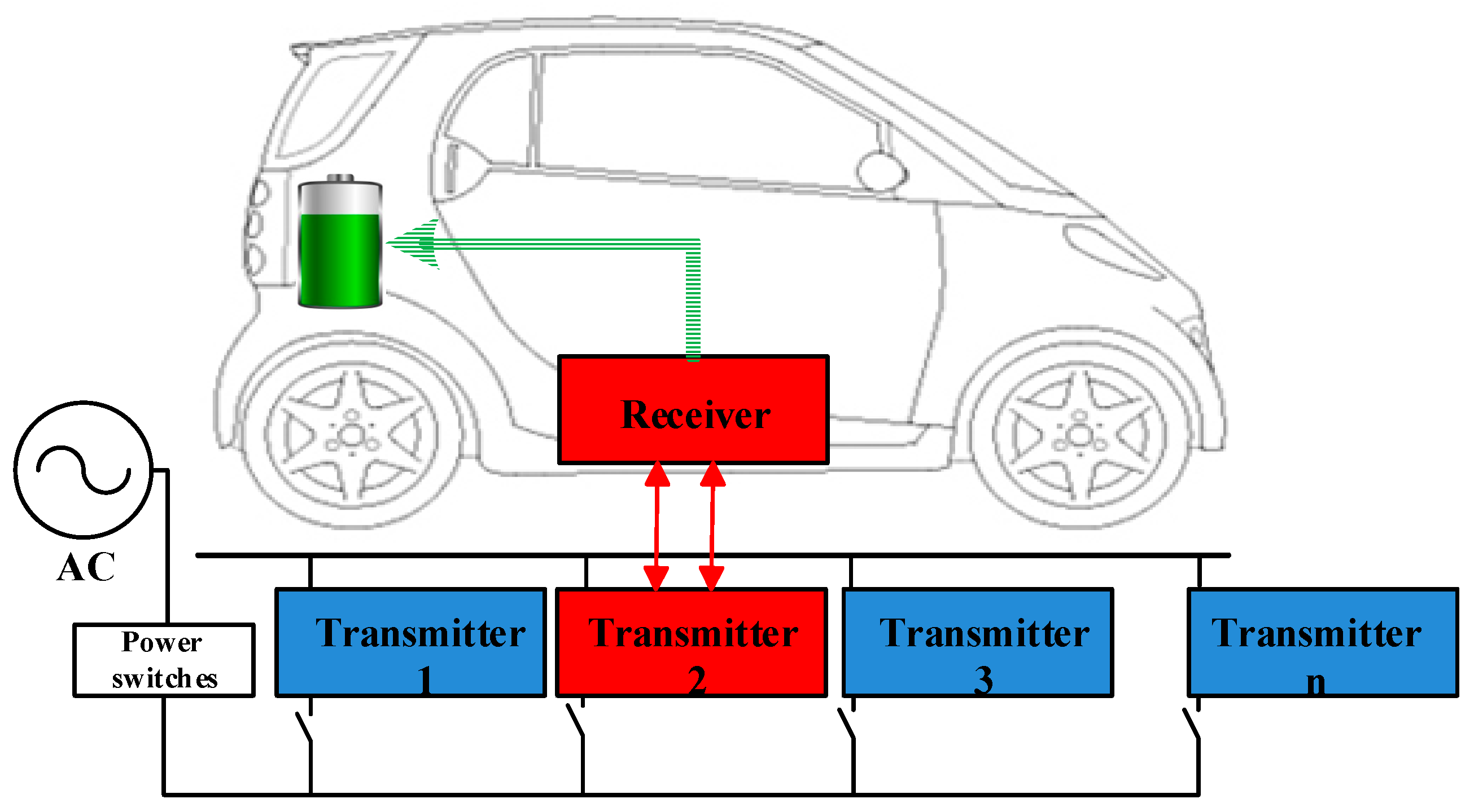
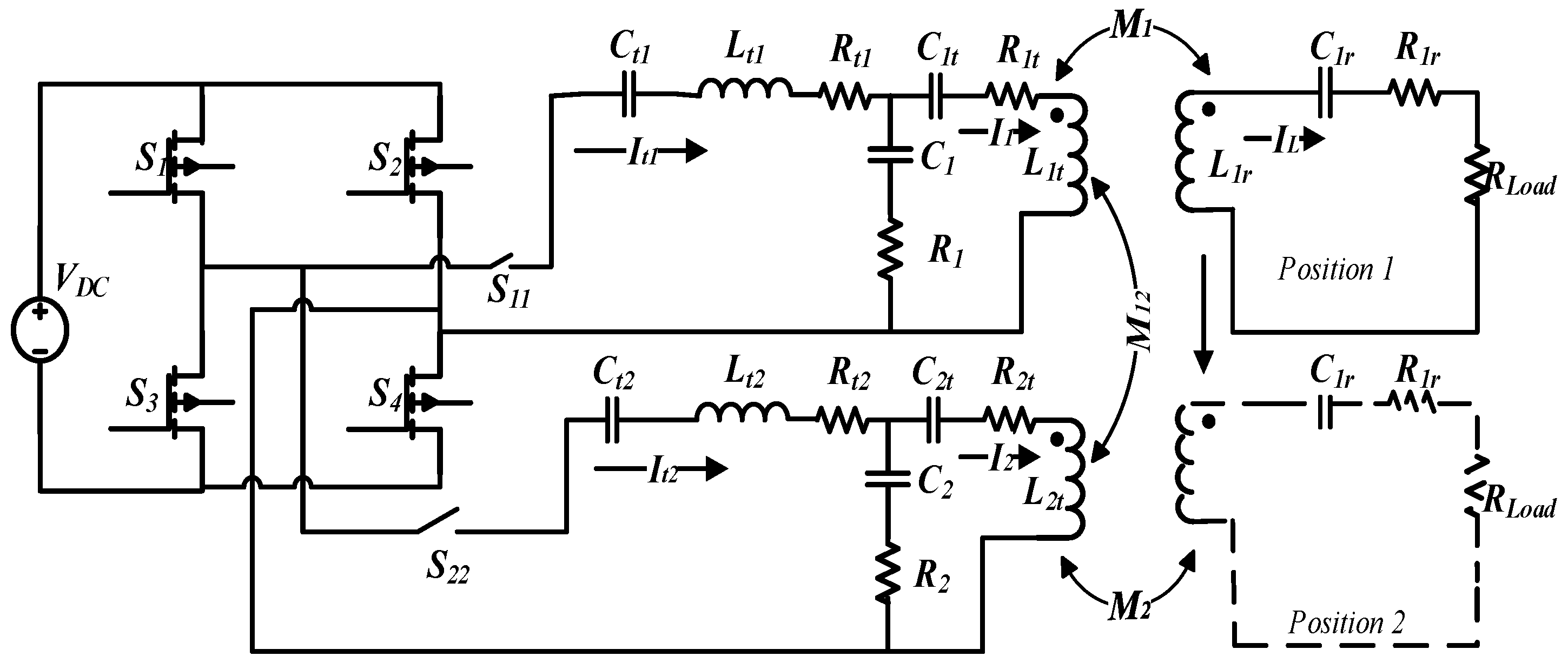
2. DWPT System Model
3. Coil Design and Simulation
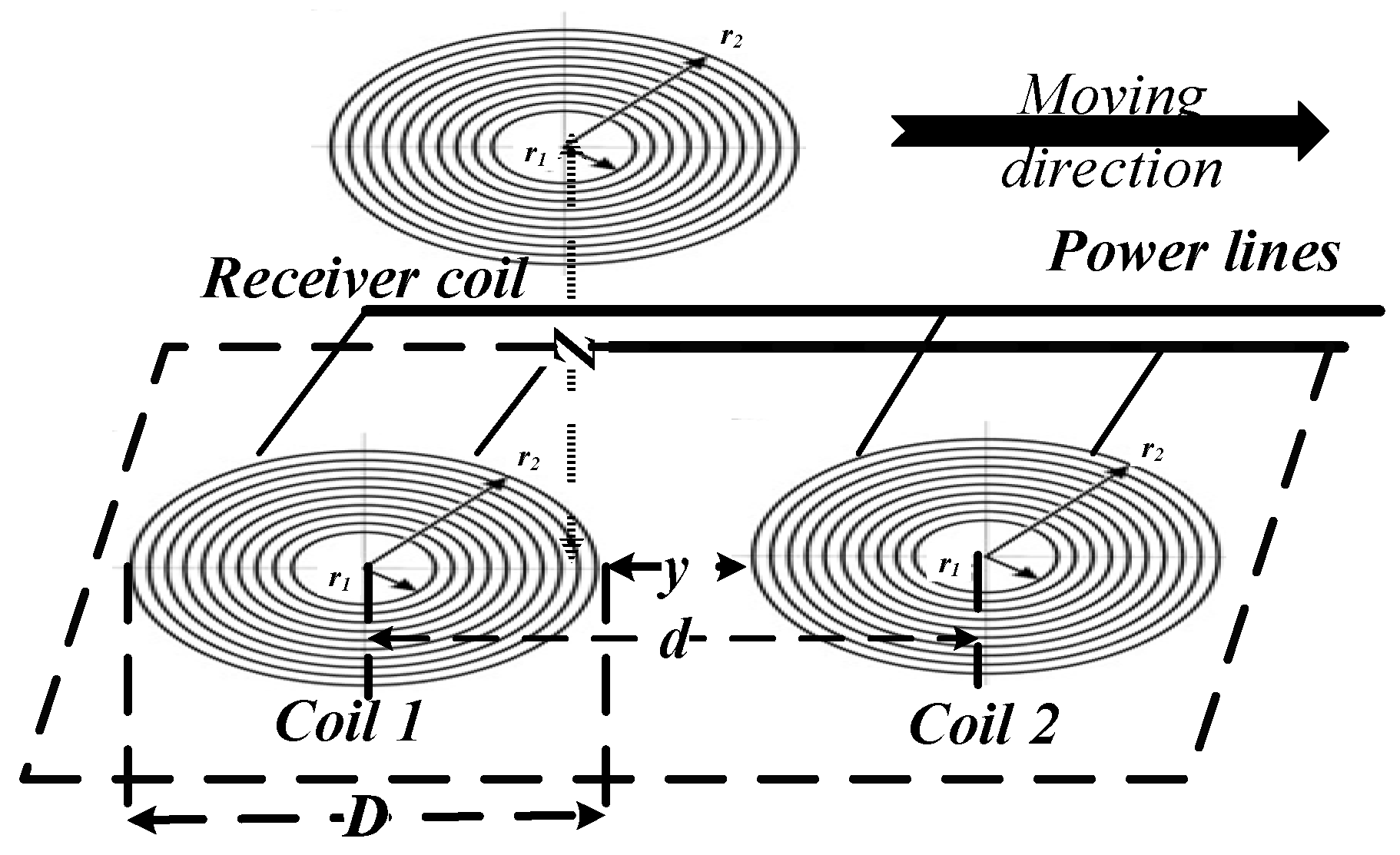
3.1. Description of Coil Design
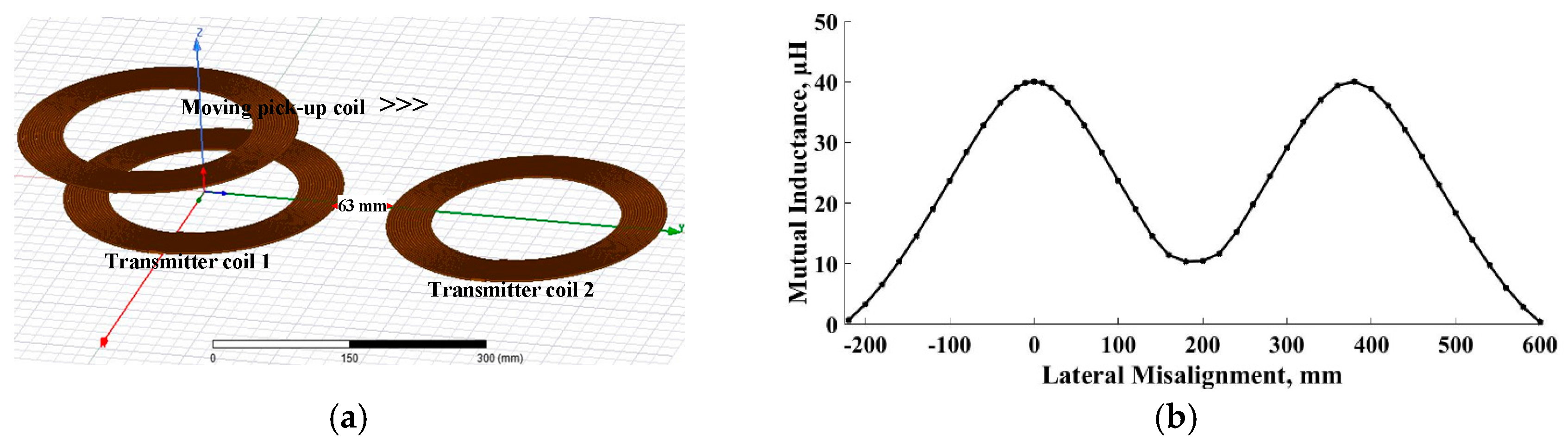
3.2. Simulation Results and Analysis
3.2.1. Case 1: Comparison of Self and Mutual Inductances
3.2.2. Case 2: Identification of Proper Distance between Transmitter Coils
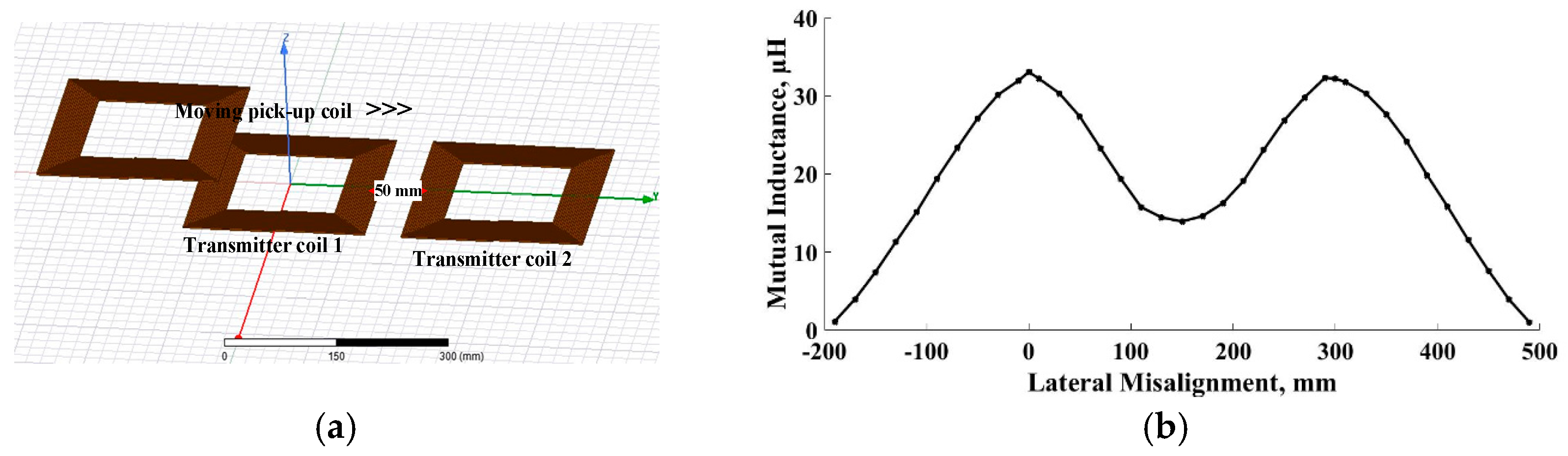
3.2.3. Case 3: Observation of Mutual Inductance Change with Respect to Lateral Misalignment
4. Practical Study on Variable Mutual Inductance
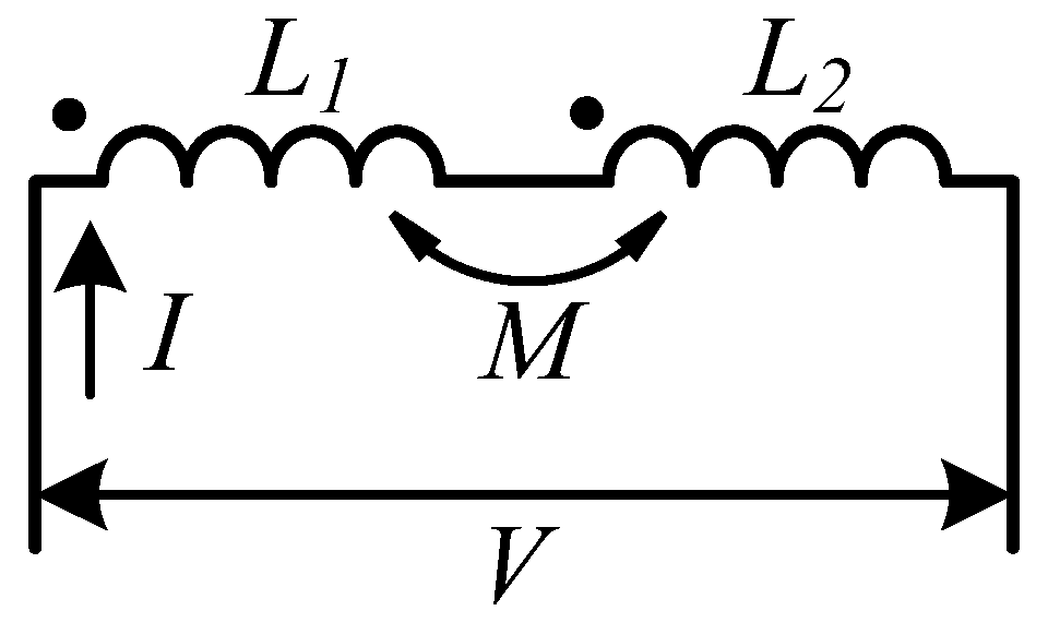
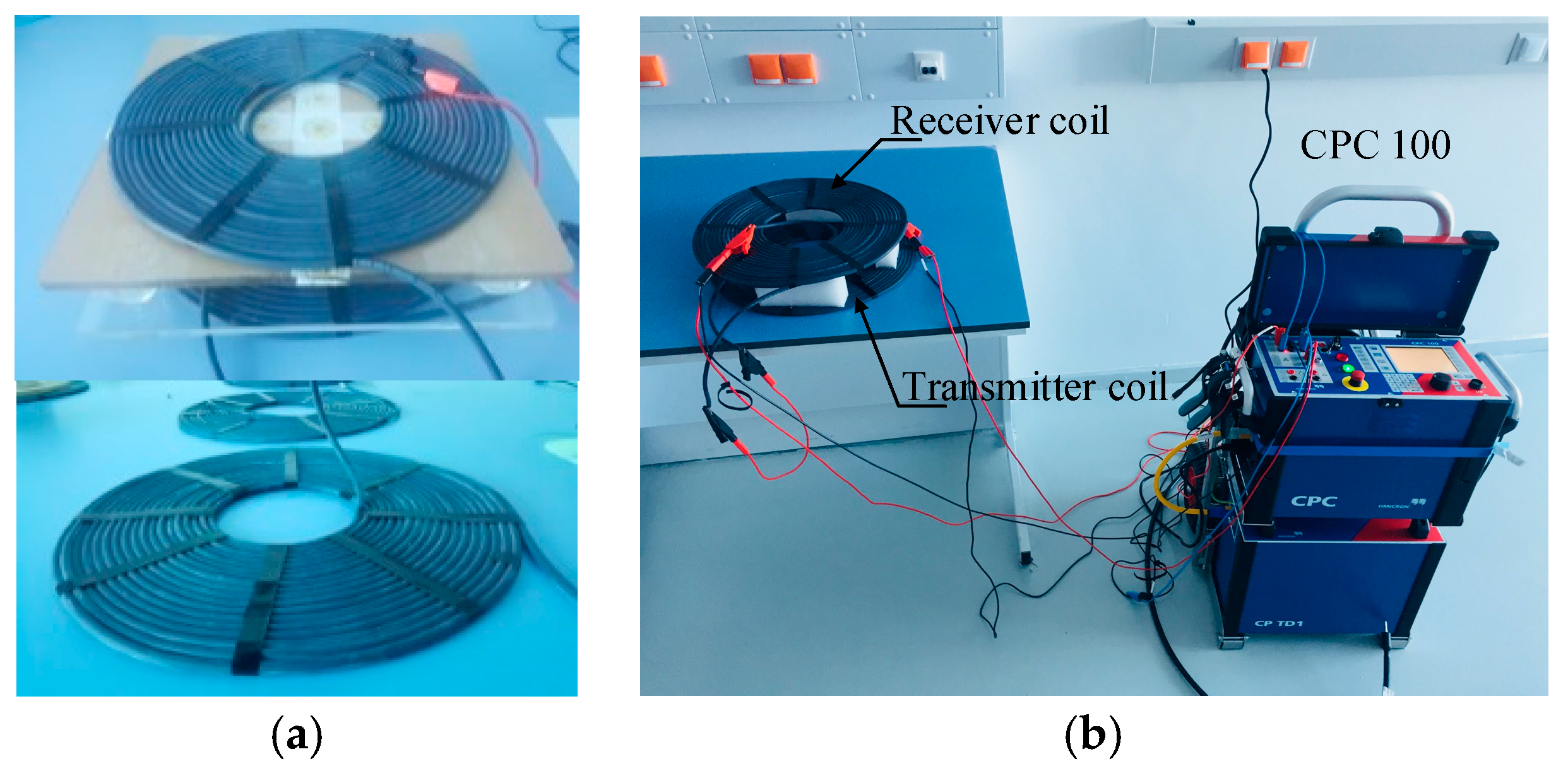
4.1. Method for Measuring Mutual Inductance
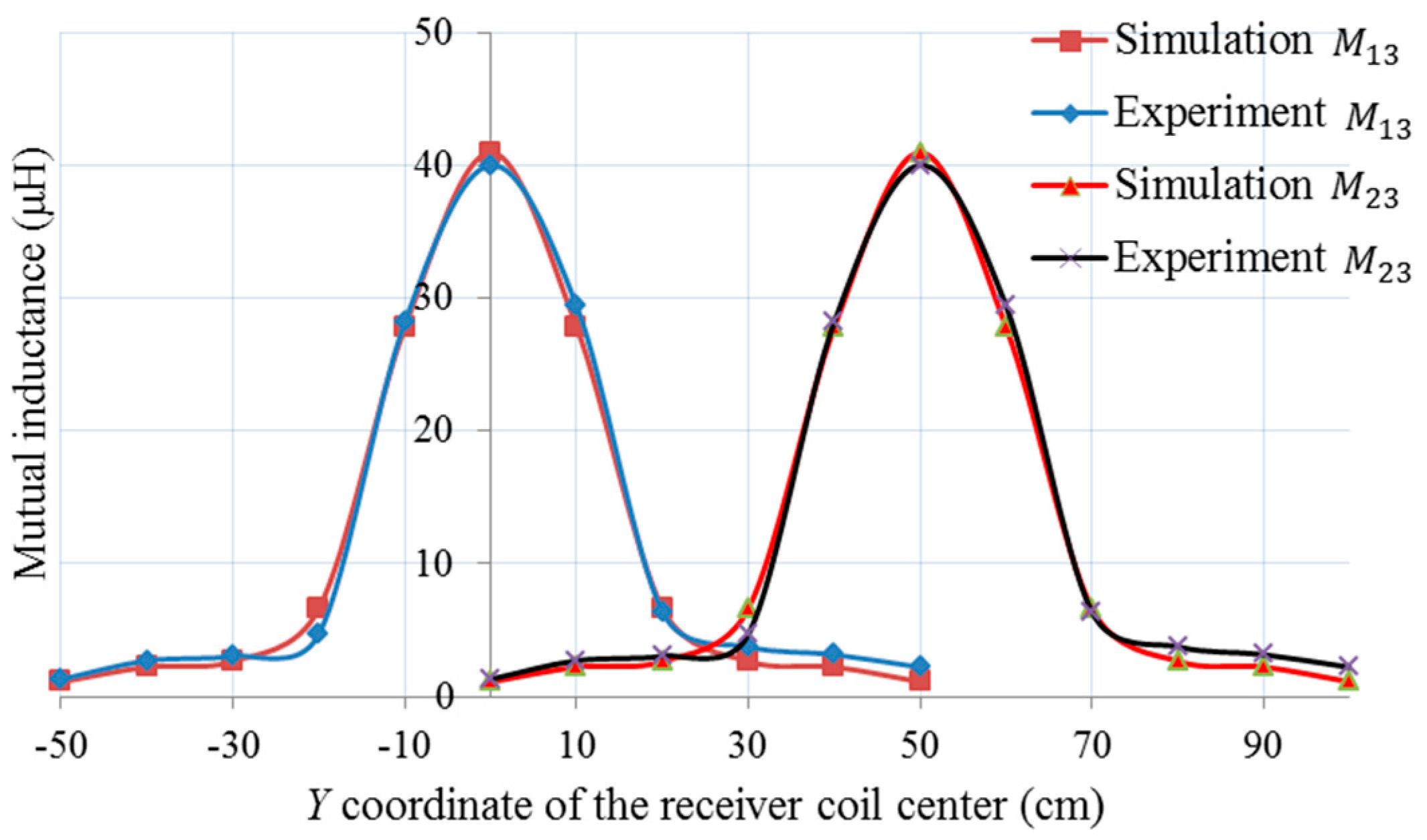
4.2. Simulation and Experiment Results
5. Dynamic WPT Simulation
5.1. DWPT Simulation
5.2. Short Discussion
6. Conclusions
Author Contributions
Conflicts of Interest
References
- Mi, C.C.; Buja, G.; Choi, S.Y.; Rim, C.T. Modern Advances in Wireless Power Transfer Systems for Roadway Powered Electric Vehicles. IEEE Trans. Ind. Electron. 2016, 63, 6533–6545. [Google Scholar] [CrossRef]
- Choi, S.Y.; Gu, B.W.; Jeong, S.Y.; Rim, C.T. Advances in Wireless Power Transfer Systems for Roadway-Powered Electric Vehicles. IEEE J. Emerg. Sel. Top. Power Electron. 2015, 3, 18–36. [Google Scholar] [CrossRef]
- Suh, I.-S.; Kim, J. Electric vehicle on-road dynamic charging system with wireless power transfer technology. In Proceedings of the 2013 International Electric Machines & Drives Conference, Chicago, IL, USA, 12–15 May 2013; pp. 234–240. [Google Scholar] [CrossRef]
- Buja, G.; Bertoluzzo, M.; Dashora, H.K. Lumped Track Layout Design for Dynamic Wireless Charging of Electric Vehicles. IEEE Trans. Ind. Electron. 2016, 63, 6631–6640. [Google Scholar] [CrossRef]
- Platt, J. IEEE-USA Today’s Engineer. Available online: http://te.ieeeusa.org/2010/Aug/electric-vehicles.asp (accessed on 18 November 2017).
- Hu, X.; Murgovski, N.; Johannesson, L.M.; Egardt, B. Optimal Dimensioning and Power Management of a Fuel Cell/Battery Hybrid Bus via Convex Programming. IEEE/ASME Trans. Mechatron. 2015, 20, 457–468. [Google Scholar] [CrossRef]
- Hu, X.; Li, S.E.; Yang, Y. Advanced Machine Learning Approach for Lithium-Ion Battery State Estimation in Electric Vehicles. IEEE Trans. Transp. Electrif. 2016, 2, 140–149. [Google Scholar] [CrossRef]
- Hu, X.; Zou, C.; Zhang, C.; Li, Y. Technological Developments in Batteries: A Survey of Principal Roles, Types, and Management Needs. IEEE Power Energy Mag. 2017, 15, 20–31. [Google Scholar] [CrossRef]
- Sallan, J.; Villa, J.; Llombart, A.; Sanz, J. Optimal Design of ICPT Systems Applied to Electric Vehicle Battery Charge. IEEE Trans. Ind. Electron. 2009, 56, 2140–2149. [Google Scholar] [CrossRef]
- Covic, G.A.; Boys, J.T. Modern Trends in Inductive Power Transfer for Transportation Applications. IEEE J. Emerg. Sel. Top. Power Electron. 2013, 1, 28–41. [Google Scholar] [CrossRef]
- Sanchez-Sutil, F.; Hernandez, J.C.; Tobajas, C. Overview of Electrical Protection Requirements for Integration of a Smart DC Node with Bidirectional Electric Vehicle Charging Stations into Existing AC and DC Railway Grids. Electr. Power Syst. Res. 2015, 122, 104–118. [Google Scholar] [CrossRef]
- Hernandez, J.C.; Sutil, F.S.; Vidal, P.G. Protection of a Multiterminal DC Compact Node Feeding Electric Vehicles On Electric Railway Syst. Secondary Distribution Networks, and PV Systems. Turk. J. Electr. Eng. Comput. Sci. 2016, 24, 3123–3143. [Google Scholar] [CrossRef]
- Zhang, W.; Wong, S.-C.; Tse, C.K.; Chen, Q. An Optimized Track Length in Roadway Inductive Power Transfer Systems. IEEE J. Emerg. Sel. Top. Power Electron. 2014, 2, 598–608. [Google Scholar] [CrossRef]
- Waffenschmidt, E.; Staring, T. Limitation of inductive power transfer for consumer applications. In Proceedings of the 13th European Conference on Power Electronics and Applications (EPE ′09), Barcelona, Spain, 8–10 September 2009; pp. 1–10. [Google Scholar]
- Liu, X.; Hui, S. Simulation Study and Experimental Verification of a Universal Contactless Battery Charging Platform With Localized Charging Features. IEEE Trans. Power Electron. 2007, 22, 2202–2210. [Google Scholar] [CrossRef]
- Chen, Q.; Wong, S.C.; Tse, C.K.; Ruan, X. Analysis, Design, and Control of a Transcutaneous Power Regulator for Artificial Hearts. IEEE Trans. Biomed. Circuits Syst. 2009, 3, 23–31. [Google Scholar] [CrossRef] [PubMed]
- Sato, F.; Nomoto, T.; Kano, G.; Matsuki, H.; Sato, T. A New Contactless Power-Signal Transmission Device for Implanted Functional Electrical Stimulation (FES). IEEE Trans. Magn. 2004, 40, 2964–2966. [Google Scholar] [CrossRef]
- Villa, J.; Llombart, A.; Sanz, J.; Sallan, J. Practical Development of a 5 kW ICPT System SS Compensated with a Large Air gap. In Proceedings of the 2007 IEEE International Symposium on Industrial Electronics, Vigo, Spain, 4–7 June 2007. [Google Scholar] [CrossRef]
- Kim, J.; Kim, J.; Kong, S.; Kim, H.; Suh, I.-S.; Suh, N.P.; Cho, D.; Kim, J.; Ahn, S. Coil Design and Shielding Methods for a Magnetic Resonant Wireless Power Transfer System. Proc. IEEE 2013, 101, 1332–1342. [Google Scholar] [CrossRef]
- Zhu, Q.; Wang, L.; Guo, Y.; Liao, C.; Li, F. Applying LCC Compensation Network to Dynamic Wireless EV Charging System. IEEE Trans. Ind. Electron. 2016, 63, 6557–6567. [Google Scholar] [CrossRef]
- Zaheer, A.; Neath, M.; Beh, H.Z.Z.; Covic, G.A. A Dynamic EV Charging System for Slow Moving Traffic Applications. IEEE Trans. Transp. Electrif. 2017, 3, 354–369. [Google Scholar] [CrossRef]
- Song, K.; Zhu, C.; Koh, K.-E.; Kobayashi, D.; Imura, T.; Hori, Y. Modeling and design of dynamic wireless power transfer system for EV applications. In Proceedings of the IECON 2015—41st Annual Conference of the IEEE Industrial Electronics Society, Yokohama, Japan, 9–12 November 2015. [Google Scholar] [CrossRef]
- Tavakoli, R.; Pantic, Z. Analysis, Design and Demonstration of a 25-kW Dynamic Wireless Charging System for Roadway Electric Vehicles. IEEE J. Emerg. Sel. Top. Power Electron. 2017, 1. [Google Scholar] [CrossRef]
- Maglaras, L.A.; Topalis, F.V.; Maglaras, A.L. Cooperative approaches for dymanic wireless charging of Electric Vehicles in a smart city. In Proceedings of the 2014 IEEE International Energy Conference (ENERGYCON), Cavtat, Croatia, 13–16 May 2014. [Google Scholar] [CrossRef]
- Lukic, S.; Pantic, Z. Cutting the Cord: Static and Dynamic Inductive Wireless Charging of Electric Vehicles. IEEE Electr. Mag. 2013, 1, 57–64. [Google Scholar] [CrossRef]
- Wang, Y.; Hu, X.; Yao, Y.; Liu, X.; Xu, D.; Cai, L.; Hu, B.; Hua, K. A dynamic wireless power transfer system with parallel transmitters. In Proceedings of the 2017 IEEE Transportation Electrification Conference and Expo, Asia-Pacific (ITEC Asia-Pacific), Harbin, China, 7–10 August 2017. [Google Scholar] [CrossRef]
- Jayakumar, A.; Chalmers, A.; Lie, T.T. A Review of Prospects for Adoption of Fuel Cell Electric Vehicles in New Zealand. IET Electr. Syst. Transp. 2017, 7, 259–266. [Google Scholar] [CrossRef]
- Lu, F.; Zhang, H.; Hofmann, H.; Mi, C.C. A Dynamic Charging System with Reduced Output Power Pulsation for Electric Vehicles. IEEE Trans. Ind. Electron. 2016, 63, 6580–6590. [Google Scholar] [CrossRef]
- Jeong, S.; Jang, Y.J.; Kum, D. Economic analysis of the dynamic charging electric vehicle. IEEE Trans. Power Electron. 2015, 30, 6368–6377. [Google Scholar] [CrossRef]
- Gilchrist, A.; Wu, H.; Sealy, K. Novel system for wireless in-motion EV charging and disabled vehicle removal. In Proceedings of the 2012 IEEE International Electric Vehicle Conference, Greenville, SC, USA, 4–8 March 2012; pp. 1–4. [Google Scholar] [CrossRef]
- Chopra, S.; Bauer, P. On-road contactless power transfer—Case study for driving range extension of EV. In Proceedings of the IECON 2011-37th Annual Conference of the IEEE Industrial Electronics Society, Melbourne, VIC, Australia, 7–10 November 2011; pp. 329–338. [Google Scholar] [CrossRef]
- Tesla, N. Art of Transmitting Electrical Energy through Natural Medium. U.S. Patent 1,119,732, 1905. [Google Scholar]
- Tesla, N. Apparatus for Transmitting Electrical Energy. U.S. Patent 1,119,732, 1914. [Google Scholar]
- Bolger, J.G.; Kirsten, F.A. Investigation of the Feasibility of a Dual Mode Electric Transportation System; Tech. Rep. LBL6301; Lawrence Berkeley Nat. Lab.: Berkeley, CA, USA, 1977.
- Bolger, J.G.; Green, M.I.; Ng, L.S.; Wallace, R.I. Test of the Performance and Characteristics of a Prototype Inductive Power Coupling for Electric Highway Systems; Tech. Rep. LBL7522; Lawrence Berkeley Nat. Lab.: Berkeley, CA, USA, 1978.
- Boys, J.T.; Covic, G.A. The Inductive Power Transfer Story at the University of Auckland. IEEE Circuit Syst. Mag. 2015, 15, 6–27. [Google Scholar] [CrossRef]
- Hao, H.; Covic, G.A.; Boys, J.T. A Parallel Topology for Inductive Power Transfer Power Supplies. IEEE Trans. Power Electron. 2014, 29, 1140–1151. [Google Scholar] [CrossRef]
- Miller, J.M.; Onar, O.C.; White, C.; Campbell, S.; Coomer, C.; Seiber, L.; Sepe, R.; Steyerl, A. Demonstrating Dynamic Wireless Charging of an Electric Vehicle: The Benefit of Electrochemical Capacitor Smoothing. IEEE Power Electron. Mag. 2014, 1, 12–24. [Google Scholar] [CrossRef]
- Raju, S.; Wu, R.; Chan, M.; Yue, C.P. Modeling of Mutual Coupling between Planar Inductors in Wireless Power Applications. IEEE Trans. Power Electron. 2014, 29, 481–490. [Google Scholar] [CrossRef]
- Acero, J.; Carretero, C.; Lope, I.; Alonso, R.; Lucia, O.; Burdio, J.M. Analysis of the Mutual Inductance of Planar-Lumped Inductive Power Transfer Systems. IEEE Trans. Ind. Electron. 2013, 60, 410–420. [Google Scholar] [CrossRef]
- Moghadam, M.; Zhang, R. Multiuser Wireless Power Transfer via Magnetic Resonant Coupling: Performance Analysis, Charging Control, and Power Region Characterization. IEEE Trans. Signal Inf. Process. Netw. 2016, 2, 72–83. [Google Scholar] [CrossRef]
- Yang, G.; Moghadam, M.; Zhang, R. Magnetic beamforming for wireless power transfer. In Proceedings of the 2016 IEEE International Conference on Acoustics, Speech and Signal Processing (ICASSP), Shanghai, China, 20–25 March 2016; pp. 3936–3940. [Google Scholar] [CrossRef]
- Nagendra, G.R.; Covic, G.A.; Boys, J.T. Determining the Physical Size of Inductive Couplers for IPT EV Systems. IEEE J. Emerg. Sel. Top. Power Electron. 2014, 2, 571–583. [Google Scholar] [CrossRef]
- Rakhymbay, A.; Bagheri, M.; Lu, M. A Simulation Study on Four Different Compensation Topologies in EV Wireless Charging. In Proceedings of the IEEE International Conference on Sustainable Energy Engineering and Application (ICSEEA), Jakarta, Indonesia, 23–24 October 2017. [Google Scholar]
- Kan, T.; Nguyen, T.-D.; White, J.C.; Malhan, R.K.; Mi, C.C. A New Integration Method for an Electric Vehicle Wireless Charging System Using LCC Compensation Topology: Analysis and Design. IEEE Trans. Power Electron. 2017, 32, 1638–1650. [Google Scholar] [CrossRef]
- Lu, F.; Zhang, H.; Hofmann, H.; Mi, C.C. An Inductive and Capacitive Integrated Coupler and Its LCL Compensation Circuit Design for Wireless Power Transfer. IEEE Trans. Ind. Appl. 2017, 53, 4903–4913. [Google Scholar] [CrossRef]
- Liu, C.; Ge, S.; Li, H.; Guo, Y.; Cai, G. Double-LCL resonant compensation network for electric vehicles wireless power transfer: Experimental study and analysis. IET Power Electron. 2016, 9, 2262–2270. [Google Scholar] [CrossRef]
- Zhu, G.; Gao, D.; Wang, S.; Chen, S. Misalignment tolerance improvement in wireless power transfer using LCC compensation topology. In Proceedings of the 2017 IEEE PELS Workshop on Emerging Technologies: Wireless Power Transfer (WoW), Chongqing, China, 20–22 May 2017; pp. 1–7. [Google Scholar] [CrossRef]
- Greenhouse, H. Design of Planar Rectangular Microelectronic Inductors. IEEE Trans. Parts Hybrids Packag. 1974, 10, 101–109. [Google Scholar] [CrossRef]
- Yu, D.; Han, K. Self-inductance of air-core circular coils with rectangular cross section. IEEE Trans. Mag. 1987, 23, 3916–3921. [Google Scholar] [CrossRef]
- Luo, Y.; Chen, B. Improvement of Self-Inductance Calculations for Circular Coils of Rectangular Cross Section. IEEE Trans. Mag. 2013, 49, 1249–1255. [Google Scholar] [CrossRef]
- Chen, W.; Liu, C.; Lee, C.; Shan, Z. Cost-Effectiveness Comparison of Coupler Designs of Wireless Power Transfer for Electric Vehicle Dynamic Charging. Energies 2016, 9, 906. [Google Scholar] [CrossRef]
- Ongayo, D.; Hanif, M. Comparison of circular and rectangular coil transformer parameters for wireless Power Transfer based on Finite Element Analysis. In Proceedings of the 2015 IEEE 13th Brazilian Power Electronics Conference and 1st Southern Power Electronics Conference (COBEP/SPEC), Fortaleza, Brazil, 29 November–2 December 2015; pp. 1–6. [Google Scholar] [CrossRef]
- Luo, Z.; Wei, X. Analysis of Square and Circular Planar Spiral Coils in Wireless Power Transfer System for Electric Vehicles. IEEE Trans. Ind. Electron. 2018, 65, 331–341. [Google Scholar] [CrossRef]
- Babic, S.; Akyel, C. New Analytic-Numerical Solutions for the Mutual Inductance of Two Coaxial Circular Coils with Rectangular Cross Section in Air. IEEE Trans. Mag. 2006, 42, 1661–1669. [Google Scholar] [CrossRef]
- Grover, F.W. Inductance Calculation: Working Formulas and Tables; Dover: New York, NY, USA, 1946. [Google Scholar]
- Babic, S.; Sirois, F.; Akyel, C.; Girardi, C. Mutual Inductance Calculation Between Circular Filaments Arbitrarily Positioned in Space: Alternative to Grovers Formula. IEEE Trans. Mag. 2010, 46, 3591–3600. [Google Scholar] [CrossRef]
- Conway, J.T. Inductance Calculations for Noncoaxial Coils Using Bessel Functions. IEEE Trans. Mag. 2007, 43, 1023–1034. [Google Scholar] [CrossRef]
- Babic, S.; Sirois, F.; Akyel, C.; Lemarquand, G.; Lemarquand, V.; Ravaud, R. New Formulas for Mutual Inductance and Axial Magnetic Force Between a Thin Wall Solenoid and a Thick Circular Coil of Rectangular Cross-Section. IEEE Trans. Mag. 2011, 47, 2034–2044. [Google Scholar] [CrossRef]
- Ravaud, R.; Lemarquand, G.; Babic, S.; Lemarquand, V.; Akyel, C. Cylindrical Magnets and Coils: Fields, Forces, and Inductances. IEEE Trans. Mag. 2010, 46, 3585–3590. [Google Scholar] [CrossRef]
- Kavitha, M.; Bobba, P.B.; Prasad, D. Effect of coil geometry and shielding on wireless power transfer system. In Proceedings of the 2016 IEEE 7th Power India International Conference (PIICON), Bikaner, India, 25–27 November 2016; pp. 1–6. [Google Scholar] [CrossRef]
- Guo, Y.; Wang, L.; Liao, C.; Zhang, J.; Zhang, Y.; Zhang, Y. Conducted EMI Analysis for Switch-On Transient of Dynamic Wireless EV Charging System. In Proceedings of the 2016 IEEE Vehicle Power and Propulsion Conference (VPPC), Hangzhou, China, 17–20 October 2016; pp. 1–4. [Google Scholar] [CrossRef]


| Parameter | Transmitter & Receiver Coils |
|---|---|
| Number of turns | 18 |
| Inner diameter | 140 mm |
| Conductor diameter | 4 mm |
| Turn spacing | 3 mm |
| Outer diameter | 400 mm |
| Coil Type | Simulation Results | Experiment Results |
|---|---|---|
| Transmitter coil | 86.8 μH | 93.4 μH |
| Receiver coil | 86.8 μH | 90.7 μH |
| Position Number | Receiver Coil Center Coordinates, cm | Mutual Inductance (Experiment), μH | Mutual Inductance (Simulation), μH |
|---|---|---|---|
| 1 | (0, −50, 6) | 1.30 | 1.10 |
| 2 | (0, −40, 6) | 2.70 | 2.22 |
| 3 | (0, −30, 6) | 3.05 | 2.65 |
| 4 | (0, −20, 6) | 4.70 | 6.63 |
| 5 | (0, −10, 6) | 28.2 | 27.8 |
| 6 | (0, 0, 6) | 40 | 40.96 |
| 7 | (0, 10, 6) | 29.4 | 27.8 |
| 8 | (0, 20, 6) | 6.35 | 6.62 |
| 9 | (0, 30, 6) | 3.75 | 2.65 |
| 10 | (0, 40, 6) | 3.15 | 2.22 |
| 11 | (0, 50, 6) | 2.20 | 1.10 |
| Parameter | Value |
|---|---|
| 115.4 μH, 115.5 μH, 115.4 μH | |
| 60 mΩ, 60 mΩ, 60 mΩ | |
| 190 pF, 190 pF, 43 pF | |
| 40 μH, 40 μH | |
| 12 mΩ, 12 mΩ | |
| 190 pF, 190 pF | |
| 12 mΩ, 12 mΩ | |
| 260 pF, 260 pF | |
| 40 μH, 40 μH, 2.3 μH | |
| 15 Ω |
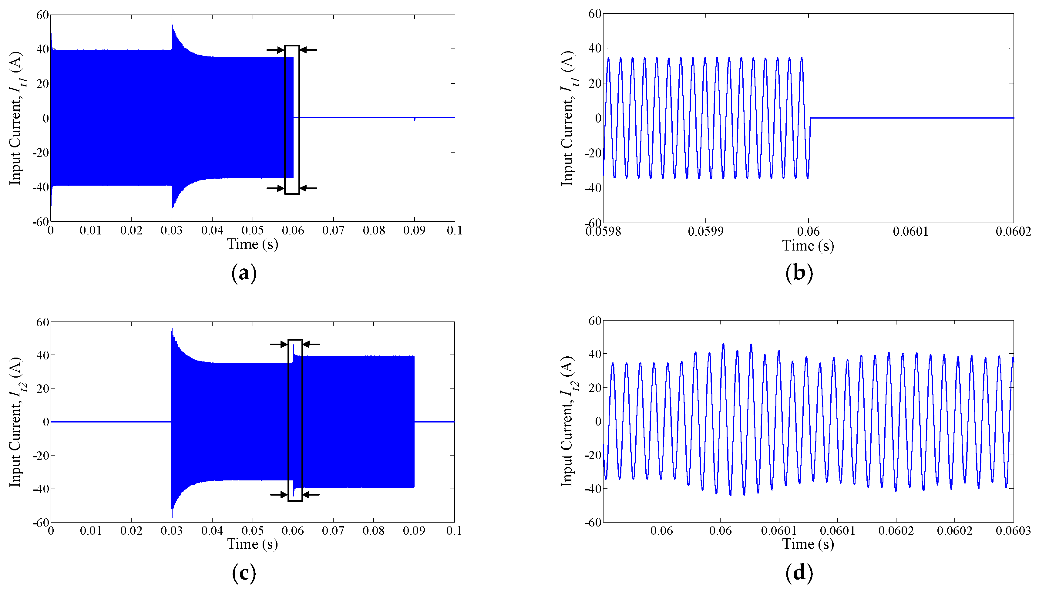
| Case | Switches ON | Time Duration |
|---|---|---|
| 1 | S11 | 0–30 ms |
| 2 | S11 and S22 | 30 ms–60 ms |
| 3 | S22 | 60 ms–90 ms |
© 2018 by the authors. Licensee MDPI, Basel, Switzerland. This article is an open access article distributed under the terms and conditions of the Creative Commons Attribution (CC BY) license (http://creativecommons.org/licenses/by/4.0/).
Share and Cite
Rakhymbay, A.; Khamitov, A.; Bagheri, M.; Alimkhanuly, B.; Lu, M.; Phung, T. Precise Analysis on Mutual Inductance Variation in Dynamic Wireless Charging of Electric Vehicle. Energies 2018, 11, 624. https://doi.org/10.3390/en11030624
Rakhymbay A, Khamitov A, Bagheri M, Alimkhanuly B, Lu M, Phung T. Precise Analysis on Mutual Inductance Variation in Dynamic Wireless Charging of Electric Vehicle. Energies. 2018; 11(3):624. https://doi.org/10.3390/en11030624
Chicago/Turabian StyleRakhymbay, Ainur, Anvar Khamitov, Mehdi Bagheri, Batyrbek Alimkhanuly, Maxim Lu, and Toan Phung. 2018. "Precise Analysis on Mutual Inductance Variation in Dynamic Wireless Charging of Electric Vehicle" Energies 11, no. 3: 624. https://doi.org/10.3390/en11030624