Abstract
Insufficient frequency regulation capability and system inertia reduction are common problems encountered in a power grid with high wind power penetration, mainly due to the reason that the rotor energy in doubly fed induction generators (DFIGs) is isolated by the grid side converters (GSCs), and also due to the randomness and intermittence of wind power which are not as stable as traditional thermal power sources. In this paper, the frequency inertia response control of a DFIG system under variable wind speeds was investigated. First, a DFIG system topology with rotor-side supercapacitor energy storage system (SCESS-DFIG) was introduced. Then a control strategy for frequency inertia response of SCESS-DFIG power grid under fluctuating wind speed was designed, with two extended state observers (ESOs) which estimate the mechanical power captured by the DFIG and the required inertia response power at the grid frequency drops, respectively. Based on one inconstant wind speed model and the SCESS-DFIG system model adopting the control strategy established, one power grid system consisting of three SCESS-DFIGs with different wind speed trends and a synchronous generator was simulated. The simulation results verified the effectiveness of the SCESS-DFIG system structure and the control strategy proposed.
1. Introduction
The basis of stable operation of a power grid system is that the balance between the power generation and the load consumption can be maintained in real time. With large-scale wind power grid-connected, the power grid frequency will be easily changed in cases of the source-network-load fluctuations or failures leading to the equilibrium destroy [1,2,3]. The main reason is, the doubly fed induction generator (DFIG) rotor speed maintains a coupling relationship with the wind speed, but it is independent of power grid frequency. As a result, it does not have the ability to respond naturally to the power grid frequency changes. While for a synchronous generator, the rotor speed will inherently vary with the grid frequency because of their directly coupling relationship, so the release (or absorption) of the rotor kinetic energy can damp the power grid frequency rapid changes. This has turned into an important problem that restricts the high penetration of wind power generation.
In order to solve the weak inertia response problem of DFIGs, many studies have been carried out and most of the literature has focused on control strategies for enhancing the inertia response ability of DFIGs at constant speeds. One study [4] clearly puts forward the concept that wind turbines participate in the power grid frequency adjustment by simulating the rotational inertia characteristic of a synchronous generator. Another study [5] deduced the relationship between the wind energy utilization coefficient and the power grid frequency in the process of virtual inertia response of wind turbines, and put forward a method to release the hidden kinetic energy of wind turbine blades. Reference [6] suggested that, if the output power of wind turbines can be controlled to have the same frequency droop characteristic as synchronous generators, it will be helpful to maintain the frequency stability of the power grid. In [7,8], the above control strategy was further improved, one variable droop coefficient or the frequency variation rate was introduced to optimize the inertia response characteristic. However, the above control methods only rely on the rotor kinetic energy to provide the inertia response power, as a result the second frequency dip often occur. Load reduction control methods were proposed in literature [9,10,11,12,13], generally by tracking the sub-optimal power curve or keeping additional power residues through pitch controls as the reserved power for better system frequency inertia response. Another study [14] proposed a control method utilizing the rotor kinetic energy to provide the inertia response energy in short time and the reserved power for the paddle reduction, to combine the inertia response with the primary frequency modulation. In [15], the wind power-energy storage inertia at constant wind speeds at wind field level was defined, and the energy storage capacity demands for increasing the inertia response of a wind farm was analyzed. In [16], a method to provide the frequency inertia response of the super capacitor and the rotor kinetic energy is proposed under the condition of wind speed stability.
The above studies have worked in detail on improving the power grid frequency inertia response ability of wind turbines under the constant wind speed. However, compared to the controls in constant wind speed conditions, the inertia response control under variable wind speeds is obviously more complex, and there are few studies addressing this problem. This paper studied the following three problems: (1) the effects of wind speed variation on the inertia response time constant of a wind turbine; (2) the instantaneous acquisition of mechanical powers which cannot be directly sampled and monitored; (3) different variation of wind speed have different effects on the inertia time constant and the control is need to be treated in different ways. In order to solve the above three problems, a DFIG system topology with rotor-side supercapacitor energy storage system (SCESS-DFIG) was introduced, and extended state observers (ESOs) were built to realize a frequency inertia control strategy for the SCESS-DFIG power grid under wind speed changes. In this control strategy, the instantaneous mechanical power in the wind turbine needs to be captured, but which is a fuzzy variable that cannot be measured directly. Therefore, an ESO estimating the mechanical power captured by the DFIG was firstly established based on the sensor sampling in the rotor-side converter (RSC). ESO is a nonlinear observer and has been extensively used in various fields of electrical engineering [17,18,19]. Then the energy changes caused by wind speed was divided as frequency ‘damping energy’, ‘underdamping energy’, and ‘overdamping energy’. In the process of the inertia response control, the grid frequency damping energy was to be preserved, and the underdamping energy was to be compensated by the rotor or the supercapacitor energy storage, and the overdamping power was to be absorbed by the rotor. At the same time, another ESO was built to estimate the damping power required for the inertia response at grid frequency drops by using the grid-side converter (GSC) sampling. In this way, the influence of voltage sampling noises on the calculations of inertia response power and df/dt can be avoided. In the system simulation in MATLAB/Simulink, the wind speed model was established which classifying the wind components as basic wind, gust, gradient wind and random wind, and the complete models of wind turbine, DFIG, DC boost/buck converter, and supercapacitor energy storage were developed. Based on these models, one power grid system consisting of three SCESS-DFIGs with different wind speed trends and a synchronous generator was simulated. The wind speed trends included speed sudden drops, reciprocating speed fluctuation, and sudden speed increases.
2. Analysis of SCESS-DFIGs
2.1. Instantaneous Power Adjustment Principle of SCESS-DFIGs
The main choosing criteria for wind farm locations include the mean wind speed, the wind consistency and the predominant wind direction. There is no specific requirement for instantaneous wind speed changes, but which has great impacts on the wind turbine frequency responses and the grid stability. The relationship between the wind speed Vwind and the generator speed can be expressed as
where R is the blade radius, λ is the tip speed ratio, the ωr is the electric angular velocity of the generator rotor, the pD is the pair number of the generator poles, and the N is the speed ratio between the turbines and the generator rotor.
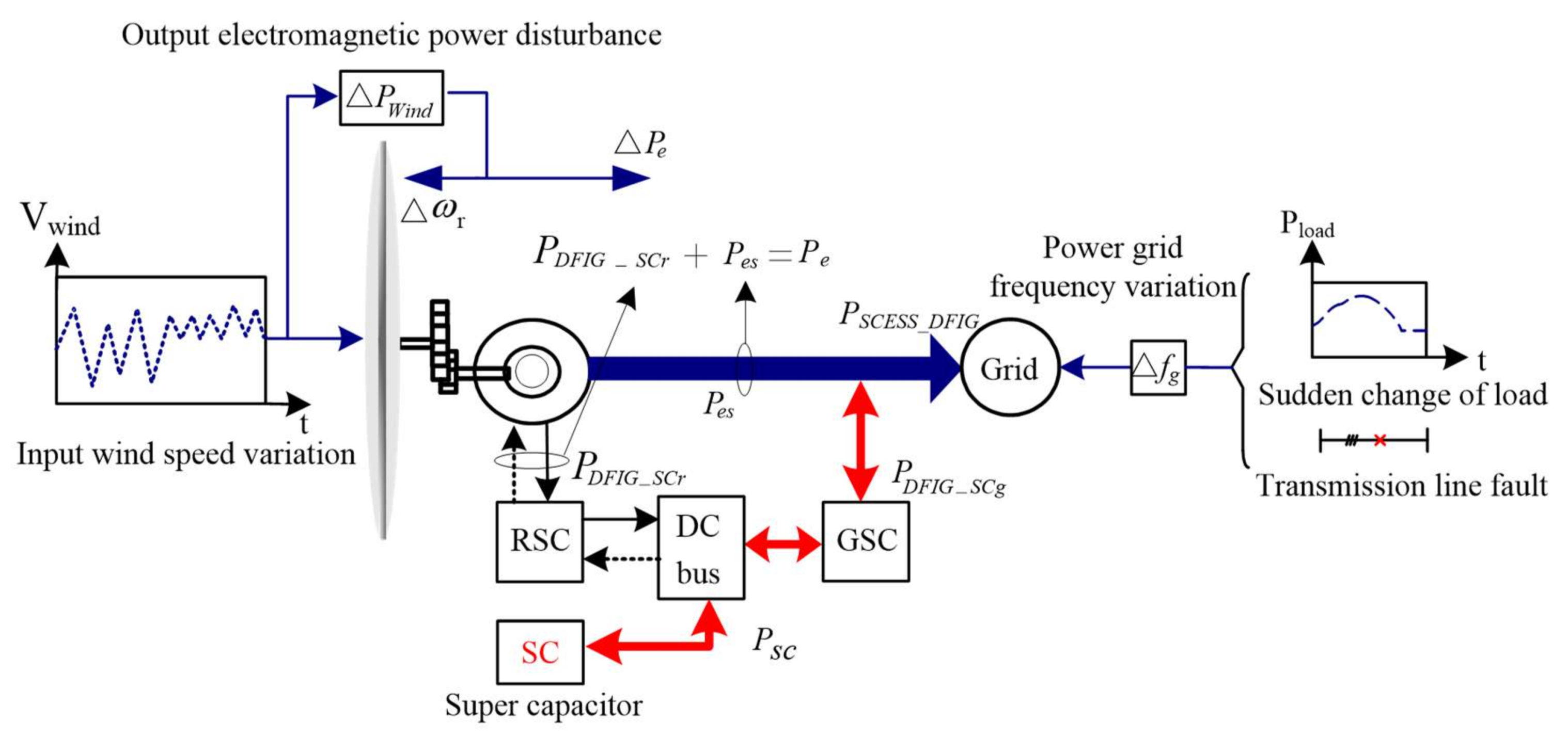
Equation (1) indicates that in the process of wind power generation, there is a coupling relationship between the rotor speed and the wind speed, and there is no direct coupling relationship between the rotor speed and the grid frequency. As shown in Figure 1, when the power system frequency changes, DFIG rotor speed and system frequency are decoupled, so there is no damping effect for the power grid frequency changes. Due to the wind changes, there will be a disturbance power ∆Pwind functioning on the DFIG and causing the rotor speed changes. In this situation, if traditional maximum power point tracking (MPPT) control is adopted, the rotor speed change will lead to the changes of output electric power Pe. When the disturbance power has the same changing tendency as the power grid frequency, the underdamping effect will be caused, which will aggravate the power grid frequency changes and possibly destroy the stability of the power system.
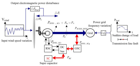
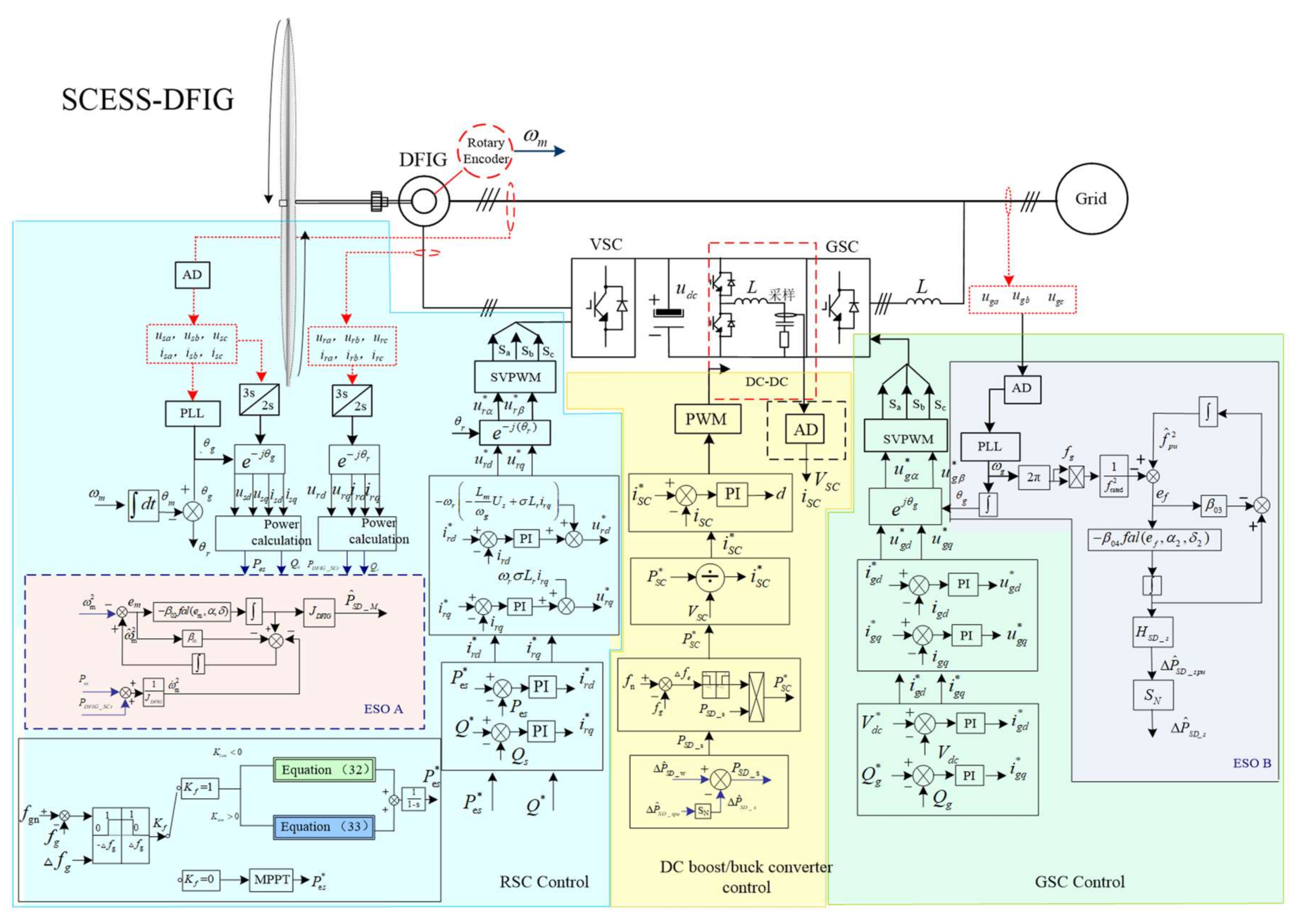
Figure 1.
The topology of a doubly fed induction generator system with rotor-side supercapacitor energy storage system (SCESS-DFIG) grid with external power disturbances. RSC: rotor-side converter; SC: super capacitor; GSC: grid-side converter.
In order to increase the inertia response capability of wind turbines and to eliminate the power disturbance caused by the wind characteristics, and to provide stable and controllable inertia response power as thermal power generation when the power grid frequency changes, one SCESS-DFIG topology is proposed as shown in Figure 1, which is used to study the frequency inertia response control strategy under the power grid frequency changes. The rotor-side back-to-back double- pulse-width modulation (PWM) converter is equipped with a DC boost/buck circuit and a supercapacitor energy storage device. Thus, the SCESS-DFIG output power will no longer be constrained strongly by wind speed like the traditional DFIGs. The SCESS-DFIG output power PSCESS_DFIG can be adjusted in a certain range by coordinating power controls, which provides a feasible channel for the inertia response control. Considering the short-time overload coefficient Koverload of the GSC, the SCESS-DFIG output power range is
where , , ωs is the angular velocity of the power grid, ωre is Electric angular velocity of rotor rotation, ωm_min is the minimum value of rotor electric angular velocity.
2.2. Definition of SCESS-DFIG Inertia Considering Wind Speed Varing
In power systems, the inertia time constant H is generally used to designate the inertia influence on the dynamic behaviors for a grid-connected generator.
where EK represents the kinetic energy stored in the rotor of a synchronous generator at the rated speed, SN represents the rated power of the synchronous generator, J represents the moment of inertia, represents the rated speed of the synchronous generator (, equal to the angular frequency of the power grid).
For the SCESS-DFIG system, the energy for the grid frequency inertia response mainly comes from the self-control of the wind turbine like pitch control, or comes from rotor kinetic energy releasing, or the energy stored in supercapacitors. In the process of the inertia response, wind speed variation will result the change of DFIG mechanical energy captured, and will affect its impact in the grid frequency inertia response. The mechanical power change of the wind turbine will lead to the imbalance between the DFIG input mechanical power and the output power. It is assumed that the inertia response time is t, then the power relationship (4) can be expressed as
where Pe is the change of DFIG output electric power caused by the wind speed variation, ωr0 corresponds to the initial value of the rotor angular velocity, ωrt corresponds to the rotor angular velocity at the time t, JDFIG is the moment of inertia of the DFIG rotor, Ewind_e is DFIG output energy variation, and ∆Eωr is DFIG rotor kinetic energy variation.
According to the Equations (3) and (4), the equivalent inertia time constant HSD of the SCESS_DFIG system under variable wind speed can be obtained as
In Equation (5), ESCESS_DFIG is SCESS-DFIG inertia response energy, ESC is the inertia response energy provided by the supercapacitor energy storage, and EKR is SCESS-DFIG inertia response energy provided by rotor kinetic energy.
where JSD represents the virtual equivalent rotary inertia.
When the grid voltage angular frequency ωg changes, the output power of the SCESS_DFIG will vary as well, and the increment can be assumed as ΔPSD, and can be expressed as
where PSC is the inertia response power provided by the supercapacitor, ΔPKR is the instantaneous power obtained from or released by the rotor, and ΔPwind_e represents the output power difference of DFIG in the process of the inertia response, between the initial value and the value at the wind speed change, when the DFIG maintains the MPPT operating conditions.
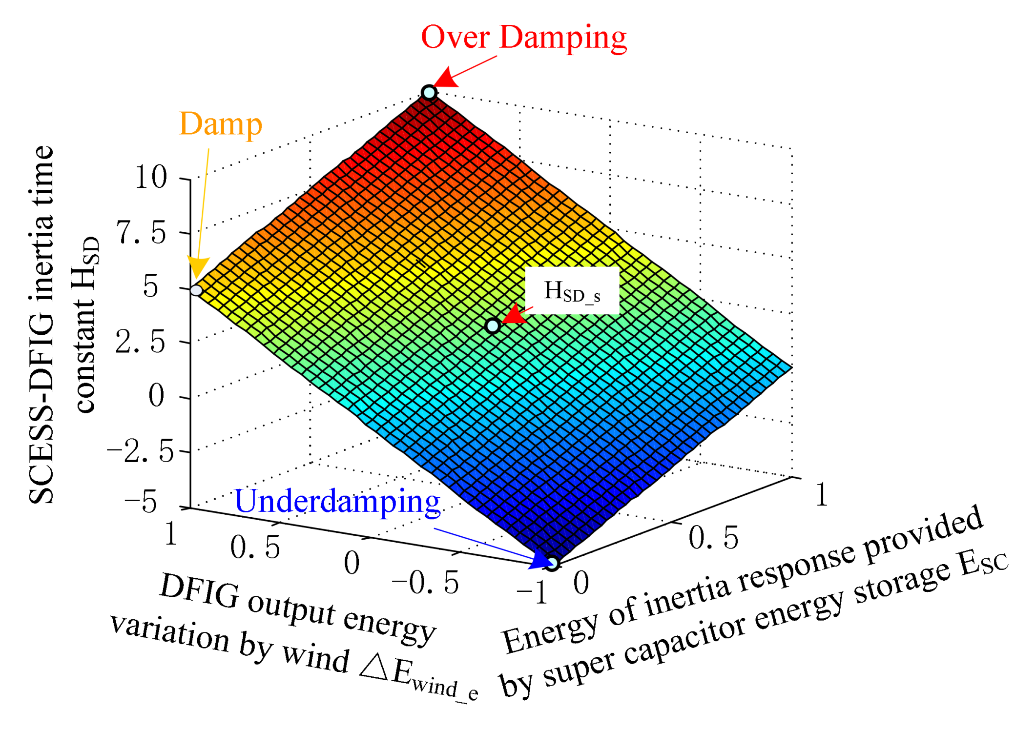
In order to evaluate the effect of wind speed variation on the inertia time HSD, the inertia response power provided by SCESS-DFIG rotor kinetic energy is not considered at first, that is, ΔEKR = 0 and ΔPKR = 0 are assumed. Equation (5) can be rewritten as
As shown in Figure 2, the inertia time constant HSD will be affected by the DFIG output power changes caused the wind speed variations, with the supercapacitors providing different inertia response energies needed. The energy changes resulted by wind speed variations can be divided into three types: damping energy, overdamping energy, and underdamping energy. If the wind speed change makes the DFIG to damp the grid frequency change, it is beneficial to the inertia response control of the DFIG. By using this energy component appropriately, the energy utilization of the supercapacitor energy storage can be optimized in the inertia response process. If the damping energy is over large, the SCESS-DFIG inertia time constant HSD will be too large also, which is unfavorable to the stability of the system frequency. If the tendency of wind speed change is the same as that of the frequency change, the frequency change will be aggravated, which is also unfavorable to the stability of the system frequency.
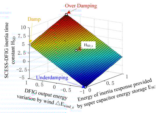
Figure 2.
The influence of wind speed on the inertia time constant HSD in SCESS-DFIG.
In order to alleviate the influence of wind speed changes on the inertia time constant HSD, it is necessary to use DFIG rotor kinetic energy or supercapacitor energy to neutralize the underdamping and overdamping energies in ΔPwind_e.
where JSD_s is the virtual equivalent rotary inertia of the SCESS-DFIG after the wind speed influence is suppressed, PSC_w is the supercapacitor power used to eliminate the effects of wind speed changes, and PKR_w is the power from the rotor kinetic energy, also used to eliminate the influence of wind speed changes.
After the wind speed variation compensation, the inertia time constant HSD_s of SCESS_DFIG can be expressed as
where ESC_w is the energy provided by the supercapacitor to eliminate the influence of wind speed changes and EKR_w is the rotor kinetic energy to eliminate the influence of wind speed changes.
The inertia constant of SCESS_DFIG, HSD_s, can be written as the following according to Equation (3)
By inserting Equation (11) into Equation (9), the ratio of SCESS_DFIG inertia response power to its rated capacity can be obtained, and its relationship with the inertia time constant and the change rate of power grid angular frequency can be expressed as
By summarizing the above equations, the inertia response power per-unit value ΔPpu can be expressed as a function of the inertia time constant HSD_s and the power grid angular velocity ωgpu in per-unit value. As the angular velocity per-unit value of the power grid is equal to the frequency per-unit value, the relationship can be obtained as (13)
Equation (13) will be used to estimate the inertia response power in ESOs. In next section, the method of estimating the input mechanical power of the DFIG will be offered as the basis for the design of the SCESS-DFIC inertia response control strategy.
3. Application of ESO in SCESS-DFIG Inertia Response Control Strategy
3.1. The Principle of ESO
A system need to exchange information with the environment during its operation. Some state variable will be passed to the outside, and some information also needs to be collected from the outside. The external variables can reflect the system internal status. In dynamic processes, the external variables can be the system output variables which containing part of the state variable information and the external input variable or control input variable information. The device for determining the internal state variables of a system based on the observations of such external variables is called a state observer (SO) [20].
The ESO is a kind of nonlinear observer which extends the total disturbance which affects the system output to a new state variable, and then estimates the state variables and the total disturbance of the system. The principle of the observer can be explained as the following:
Taking a class of uncertain nonlinear dynamic systems into account which can be expressed as
where x is the state variable, w (t) is the uncertain disturbance, t is the time, u is the control input, and b is the gain of control input. f (*) is a smoothing function of the state variable x and its derivatives . It can be extended to higher dimensional state space and converted to a dynamic system with standard single input and single output.
In Equation (15), the state xn is an extended state that is augmented to quantify the influence of uncertain disturbances. In a single extended dynamical system, both the state variables and the disturbances well as their interactions can be investigated. So an ESO for Equation (15) can be constructed as
where is the estimated value of the state xj (j = 1, 2, 3… n − 1); is the estimated value of the extended state xn; the function is the nonlinear feedback of the system (j = 1, 2, 3… n). In fact, it is unnecessary to assume that the function is continuous or discontinuous, known or unknown. As long as its real-time action x in the process is bounded and the parameter b is known, the appropriate parameter β0j always can be chosen, so that the ESO can estimate the state of the state xj and the extended state xn in real time.
In this paper, for studying of SCESS-DFIG inertia response control strategy, ESOs are constructed to estimate the mechanical power of wind turbine and the inertia response power at grid frequency varying. Both of them are used on the basis of accurate first-order ESO estimations. So an additional description of the first-order ESO is given below.
For the following nonlinear uncertain first-order systems:
the new state variables are defined as
then the new state equation is
and an ESO can be constructed as
where the expression of function is
3.2. SCESS-DFIG Mechanical Power Input Estimation Based on an ESO
The mechanical power of the rotor is an internal state, it cannot be sampled directly by using a sensor. There is a mathematical relationship between the rotor speed and the mechanical power of the wind turbine. However, during rotor speed measurement, interference factors such as acquisition noises will be introduced, so it is difficult to accurately obtain dωr/dt. At the same time, the acquisition of mechanical power cannot be reached by directly calculating the kinetic equation. In this paper, the purpose of the ESO is not to use dωr/dt, but to estimate the real-time state of the mechanical power input of the wind turbine based on the dynamic behavior of the generator. The estimated result is used as an input for the DFIG inertia response control.
PSD_m is the input mechanical power of the DFIG; Pes is the DFIG stator output electric power; PDFIG_SCr is the power of the RSC; is the mechanical power lost in the process of energy conversion. Pes + PDFIG_SCr is as marked in Figure 1. As the SCESS-DFIG GSC contains supercapacitor input power component, the power Pes + PDFIG_SCr instead of PSCESS-DFIG is used in the Equation (22).
As the equation is a nonlinear differential equation, it cannot be estimated directly by the ESO. However, dωr/dt and ωr can be transformed into one sole form by using dωr/dt to represent ωr.
Equation (23) can be rewritten as the first-order differential form of ω2m:
The power of the wind energy captured and the mechanical loss power are combined into PSD_M which is the input mechanical power of the SCESS-DFIG. Equation (24) can be organized as
In Equation (25), z1 = ω2m, z2 = PSD_M/JDFIG, input u1 = Pes + PDFIG_SCr, the input coefficient b1 = −1/JDFIG, thus the following ESO can be constructed
The estimated values of PSD_M and ω2m are and respectively. By selecting the appropriate parameters of α1, δ1, β01, β02, the ESO can accurately estimate the input mechanical power of the generator. In the process of estimation, the main parameters of the ESO-A are JDFIG, ωm, Pes and PDFIG_SCr. JDFIG is an intrinsic parameter of DFIG. ωm, Pes, and PDFIG_SCr can be calculated simply by sensing the speed, voltage, and current. As shown in Figure 3, the ESO is named as the ESO-A which is used to estimate the generator input mechanical power. The estimated value can also be invoked as a reference for generator output power control.
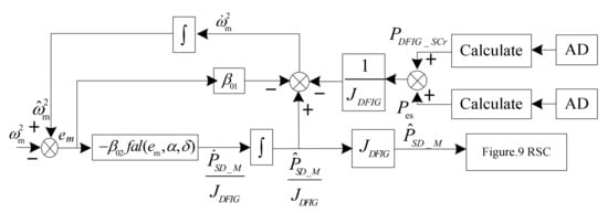
Figure 3.
Operational principle of ESO-A. AD: analog-digital.
3.3. Frequency Inertia Response Power Estimation of SCESS-DFIG Based on ESO
When the frequency of the power grid changes, the SCESS-DFIG needs to provide the inertia response power to damp the frequency change. In most literatures, no matter proportional-derivative (PD) control strategy or fuzzy control strategy were adopted, it is necessary to detect the power grid frequency f and the power grid frequency change rate df/dt.
In the sensing process of the voltage, noise interference is inevitable. So generally, a low pass filter is needed before the frequency change rate df/dt can be used, and the choice of time constant affects the df/dt filtering value seriously. An ESO can be designed to solve this problem. Figure 4 is comparison of PD control, fuzzy logic control and ESO result for power grid frequency inertia response (the parameters of PD control and the membership function of fuzzy control are given in Appendix B, Figure A1, Figure A2 and Figure A3, Table A3). Through the Equation (13), it can be found that the main control parameter of the ESO is df/dt, so it can better reflect the change of the rotor speed of the generator. When the change rate of the power grid frequency is negative, the rotor speed decreases and the power is released. When the power grid frequency rises, the rotor speed rises, absorbing the power. Traditional PD control has slow response and is susceptible to noise in the acquisition signal. The control continuity of fuzzy control is poor, and the choice of membership degree can be determined by long-term parameter detection. The ESO can be used to track the frequency change quickly, and the design is simple and easy to realize.
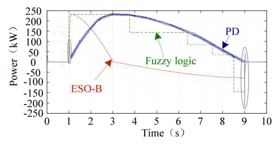
Figure 4.
Comparison of proportional-derivative (PD) control, fuzzy logic control and ESO-B result for power grid frequency inertia response.
Based on the discussion in Section 2.2, HSD_s can be considered as a fixed value. Then the Equation (13) can be rewritten as a nonlinear differential equation related to the grid frequency per-unit value. After further consolidation, we can get the state equation of the extended observer as
Equation (27) can still be rewritten as the standard first-order differential equation of the grid frequency per-uint square value f2pu as
Based on Equation (28), the extended state equation can be obtained as
In Equation (29), z1 = f2pu, z2 = PSD_spu/HSD_spu, the input u2 = 0, and the input coefficient b2 = −1/HSD_spu. Thus the following expansion SO can be constructed as
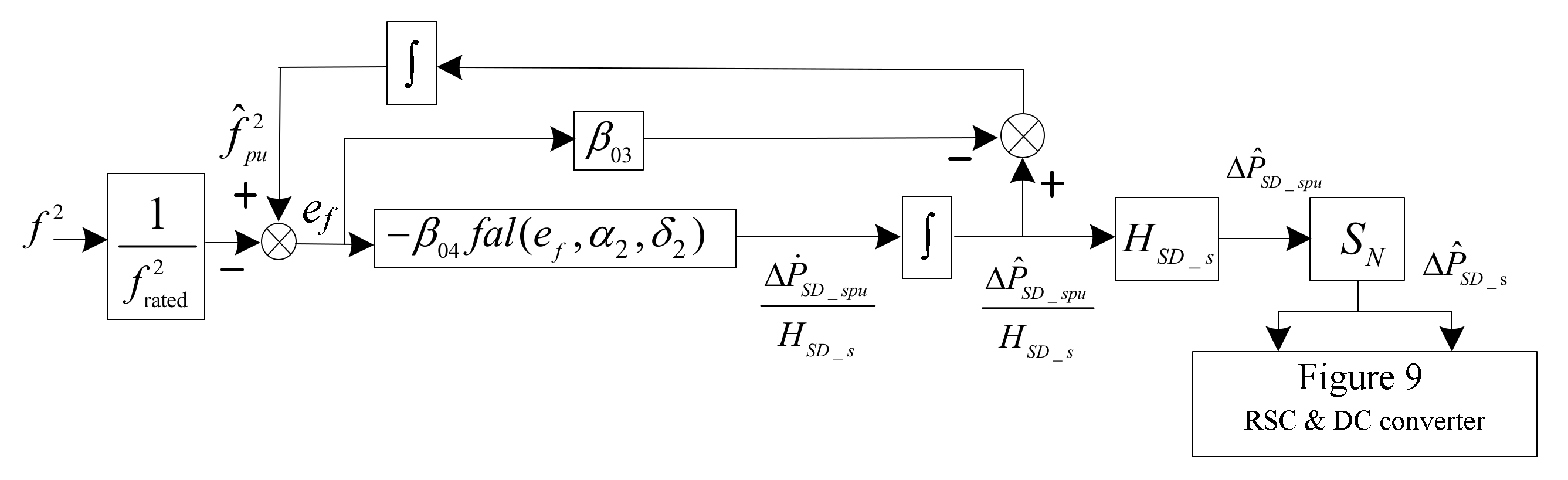
The estimated values of and are and . By selecting the appropriate parameters of α2, δ2, β03, β04, the ESO can accurately estimate the per-unit value of the inertia response power provided by SCESS-DFIG when the frequency changes. This ESO is named as the ESO-B. As shown in Figure 5, the operational principle of ESO-B. When the frequency of the power grid is used as the input of the ESO-B, the value of the power required for the power gird frequency inertia response can be estimated.
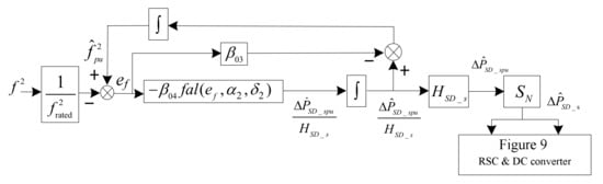
Figure 5.
Operational principle of ESO-B.
3.4. Parameter Selection of ESO
According to the literature [20,21,22,23], Equation (16) has another expression as shown in Equation (31).
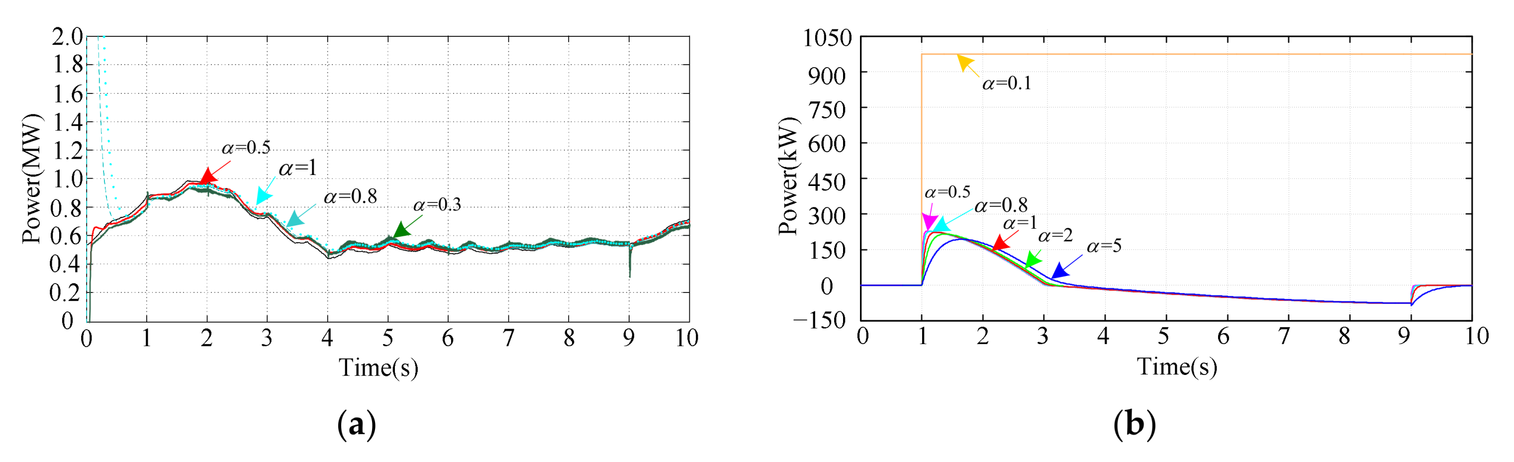
For the nth-order system parameters α1 = 1/2, α2 = 1/22, α3 = 1/23……αn−1 = 1/2n−1. Therefore, the parameter α of the first order ESO-A and ESO-B is usually selected to be 0.5. As shown in Figure 6, the estimated results of the ESO-A and the ESO-B are compared for different alpha given. We can find a better result when α = 0.5. The parameter δ is the filter factor, which is usually set to be larger than the sampling step for guaranteeing the filter performance. β01 is mainly related to the effect of estimation of state , β02 is related to the effect of estimation of extended state , β0n−1 is related to the effect of estimation of extended state . Larger β01 and β02 usually result in a faster convergence rate, albeit they might increase the risk of oscillation of the ESO’s output [22]. As shown in Figure 7a, β01, β02 too small (β01 = 10, β02 = 100) system will diverge, β01, β02 too large (β01 = 10,000, β02 = 100,000) control effect will decline, while prolonging the simulation time. As shown in Figure 7b, β03 = 1000, β04 = 20,000, it will have a better effect.
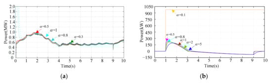
Figure 6.
Comparison of DFIG mechanical input power estimation with ESO under different parameters: (a) comparison of estimation with ESO-A under different α; (b) comparison of estimation with ESO-B under different α.
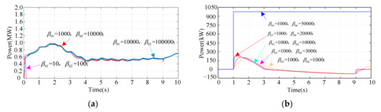
Figure 7.
Comparison of DFIG mechanical input power estimation with ESO under different parameters: (a) comparison of estimation with ESO-A under different β01, β02; (b) comparison of estimation with ESO-B under different β01, β02.
4. Frequency Variation Inertia Response Control Strategy of the SCESS-DFIG Power Grid Considering Wind Speed Change
4.1. Stratified Damping Control for Wind Speed Changes in the Power Grid Frequency Inertia Response
The effect of wind velocity variation on the inertia time constant of SCESS-DFIG has been discussed in Section 2. It is suggested that different wind speed changes have different effects on the inertia response, some are beneficial and some are harmful. When the supercapacitor energy storage system is added to provide the system inertia response power and stabilize the wind energy fluctuation, the influence of wind speed variation on SCESS-DFIG can be eliminated. However, the capacity of the supercapacitor energy storage system should be restricted to an appropriate value, as well as the capacities for GSC of DFIG. Therefore, a power control strategy was developed to coordinate the SCESS-DFIG rotor kinetic energy and the supercapacitor energy storage in this section. The enhancement of SCESS-DFIG inertia response ability was also presented by hierarchically controlling of the varying wind energy.
As shown in Figure 8 when the frequency of the power grid changes, there is a disturbance to the input power of the wind turbine caused by wind speed changes. Pe0 is the initial electric power of the inertia response. With using ESO-A to estimate the input mechanical power of DFIG, one hierarchical control of the output electric power of the generator was adopted which functioning as a wind speed filter, to eliminate the influence of wind speed variation on the frequency inertia response of the power grid, including underdamping and overdamping responses.
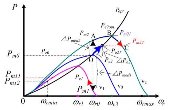
Figure 8.
Mechanical input power and electromagnetic output power curve of the DFIG under different wind speed.
The SCESS-DFIG will enter into the inertia response mode when the overlimit of the power grid frequency change has been detected. The difference between the estimated value of DFIG input mechanical power and the output electric power of generator Pe is ∆Pmed. Assume a wind speed and frequency trend determination coefficient as Kten, whose definition is
By judging the value of Kten, the relationship between ∆Pmed and the frequency change trend of the power grid can be determined, and the energy introduced by wind speed change can be determined as damping or underdamping.
Taking Figure 8 as an example to further illustrate the idea of the hierarchical control at sudden rises or falls of wind speed. In the following analysis the falls of the power grid frequency were assumed.
(1) Sudden rise of wind speed: It can be assumed that the wind speed increases to V2 from V0 in the preliminary stage. As a result, the input mechanical power of the wind turbine also changes from point O to A, with the power value suddenly increases to Pm2, which is greater than the output power Pe0 of SCESS-DFIG at the initial moment of inertia response of the generator.
In this case the determination coefficient Kten < 0, which indicating that the wind speed change has brought beneficial energy for damping the grid frequency change. However, if the wind speed rises too fast or the amplitude is too high, the overdamping power will be introduced, which will still affect the inertia response. Therefore, the output power of the generator must be limited. As shown in Equation (33), with the inertia response power estimated by the ESO-B in the GSC, the total power Pe2 of the DFIG stator and RSC at any time t2 can be limited coordinately
where Pe2 is the output power of DFIG while maintaining MPPT control. In short, when Kten < 0, the minimum output power of DFIG is Pe0 and the maximum output power is the sum of Pe0 and the estimate value .
Due to the power difference Pmed2 between mechanical power and output electric power of DFIG, its mechanical power input gradually changes from point A to B (the maximum mechanical power input of DFIG Pm21 = Pe2opt). Finally, the mechanical input power Pm22 of point C is equal to the output electric power Pe2 of the generator, the input and output power balance are achieved and the rotor speed of the generator will no longer increase. As a result of the control, the output electric power will eventually be equal to the input mechanical power of the wind turbine, and the rotor speed will not be greater than the maximum speed of ωrmax.
(2) Sudden drop of wind speed: When the inertia response occurs, if the wind speed drops from V0 to V1, the mechanical input power of DFIG decreases to Pm1. In order to eliminate the influence of wind speed, the DFIG output electric power is controlled to be Pe0. Owing to the existence of power difference -∆Pmed1, the rotor speed gradually decreased to ωr1. In order to ensure that the rotor speed is not lower than the minimum speed ωrmin, it is necessary to use the ESO-A to estimate the mechanical input power and to limit the output electric power Pe. The generator inertia response time is TJ. Assuming at a time t1, the mechanical power estimation value is , the rotor speed is ωrt1 and Pet1 is MPPT power at time t1, then the electric power output Pet1 is
Therefore, when the wind speed drops, the power curve of the output electric power will be controlled along the V1 wind speed. When the input mechanical power reaches E point, the output electric power will also be reduced to E point, so as to maintain the rotor speed.
4.2. Frequency Variation Inertia Response Control Strategy of SCESS-DFIG Power Grid Considering Wind Speed Change
The above content described the electric power control of the DFIG at wind speed variations for reducing the speed variation influence on the grid frequency responses. Furthermore, the power grid frequency inertia response control strategy of SCESS-DFIG at varying wind speeds was designed based on the establishment of ESO-A and ESO-B. As shown in Figure 9, the control strategy can be divided into three parts, including the control strategies of the GSC, of the RSC, and of the DC converter respectively.
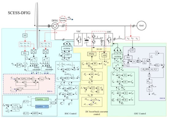
Figure 9.
A frequency inertia response control strategy for SCESS-DFIG power grid considering wind speed changes. SVPWM: space vector pulse width modulation; PI: proportional-integral.
(1) The Control Strategy of the GSC:
In the process of grid frequency inertia response control, the original control strategy of stabilizing DC bus voltage of the GSC is maintained. In the system, the grid voltages uga, ugb, ugc are directly sampled from the voltage sensors of the GSC, and the grid angular velocity ωg can be obtained through the phase-locked loop (PLL) calculation. The power grid frequency fg corresponding to ωg is used as one input of the ESO-B, which outputs the estimated per-unit value of the inertia response power of the wind turbine. The estimated power , which is the product of and the DFIG rated capacity SN, will be used in the control of the RSC and DC converter. ∆fg is the difference between the power frequency fg and the rated frequency fn, which is used as the enable signal to control the SCESS-DFIG power grid frequency inertia response.
where Kf is the starting position of the frequency inertia response of the SCESS-DFIG power grid.
(2) The Control Strategy of RSC:
The sum of stator active power Pes and rotor-side active power PDFIG_SCr are inputs of the ESO-A. Based on the sampling of the voltages and currents by sensors of DFIG, including the rotor-side voltage ura, urb, urc and current ira, irb, irc, stator-side voltage usa, usb, usc and current isa, isb, isc, the total active power of the DFIG can be calculated through the d-q coordinate transformation as
ESO-A generates the estimated input mechanical power value of the DFIG. When Kf = 1, the relationship between the change of wind speed and the change of the power grid frequency is determined by Kten. When Kten < 0, the MPPT is kept to control the DFIG. The maximum electric power limit of the generator is set as the sum of the initial electric power Pe0 and the estimated power from the GSC. When Kten > 0, the DFIG exits the MPPT control, with its output electric power is maintained as Pe0. The specific control method has been outlined in Section 4.1.
(3) The Control Strategy of DC Converter:
The DC converter realizes the energy exchange between the supercapacitor energy storage and the DC bus of the DFIG rotor side back-to-back PWM converter. Since the power of the RSC is controlled by the output electric power instructions, the control goal of the GSC is to stabilize the DC bus voltage. Therefore, the output power of the DC converter can be exchanges with the power of the GSC, and also the output power PSCESS-DFIG of SCESS-DFIG can be exchanged. The power of the DC converter PSC_t1 can be obtained from the initial output electric power Pe0, the DFIG output electric power Pet1 at the time t1, and the GSC ESO-B estimated inertia response power , as shown in
In the control process, the voltage value Vsc of the DC converter is obtained by sampling the voltage of the supercapacitor, and it is used to calculate the working current i*sc. The instantaneous working current isc from the current sensor is used as the current loop control feedback. Then the duty cycle d can be obtained in PI control, which is used as the given control signal of the DC converter.
Through the coordinated control of GSC, RSC, and the DC converter, the SCESS-DFIG can provide stable and controllable damping power when the power grid frequency changes.
5. Simulation Studies
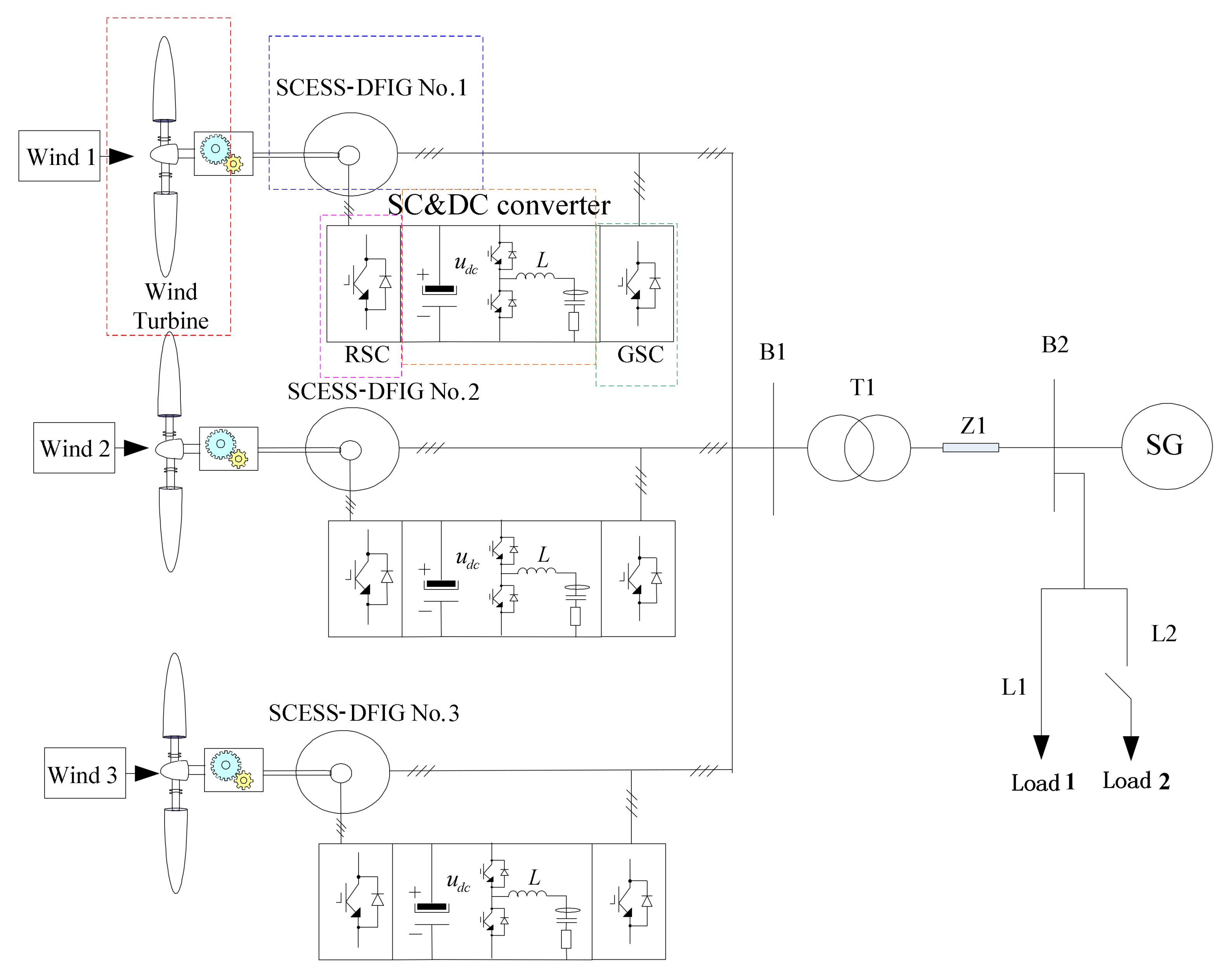
In order to verify the effectiveness of the control strategy proposed in this paper, one simulation model of the SCESS-DFIG grid consisting of wind turbine, DFIG, RSC, GSC, DC/DC converter, and supercapacitor models was constructed in MATLAB/Simulink (2014b, The MathWorks, Natick, MA, USA). The system structure and electrical parameters are shown in Figure 10 and Table A1 (Appendix A) respectively. The simulation model includes three SCESS-DFIG with the same electrical parameters, and one synchronous generator (SG), load L1 and load L2, used to verify the inertia response control strategy with the parameters being shown in Table A2 (Appendix A). Concretely, the rated power of one SCESS-DFIG is 2.5 MW, the capacity of the synchronous generator SG is 50 MW, the capacity of load L1 is 10 MW, and the capacity of L2 which is a shock load is 3 MW. The wind speed curves for the simulation inputs are shown in Figure 11, which are the compounds of the basic wind speed models as basic wind, gust, gradual wind, and stochastic wind. The initial values and the wind speed variations for each SCESS-DFIG are different. Concretely, for no. 1 SCESS-DFIG, the input wind speed drops abruptly at 1 s and rises at 3 s; for no. 2 SCESS-DFIG, the input wind speed is reciprocating wave; and for no. 3 SCESS-DFIG, the input wind speed curve has a stable start and a continuous rising change.
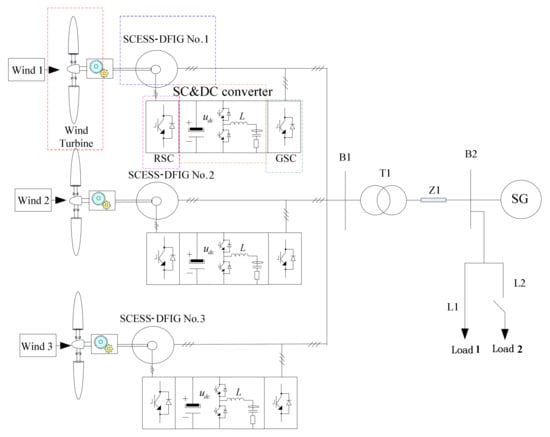
Figure 10.
Simulation system diagram. SG: synchronous generator.
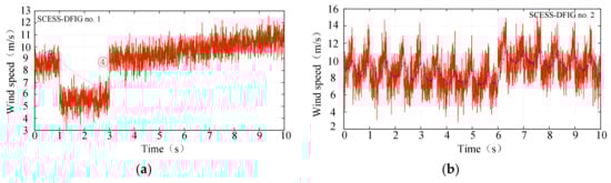
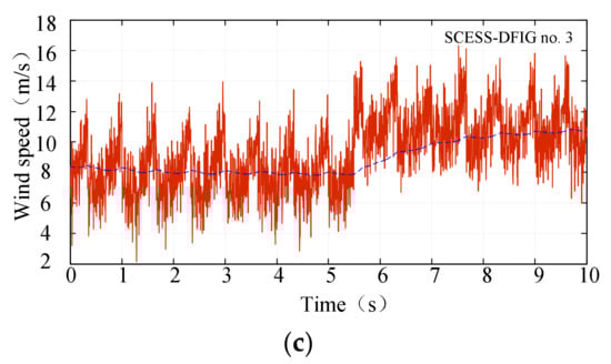
Figure 11.
Wind speed curve given for SCESS-DFIG: (a) Wind speed curve given for SCESS-DFIG no. 1; (b) Wind speed curve given for SCESS-DFIG no. 2; (c) Wind speed curve given for SCESS-DFIG no. 3.
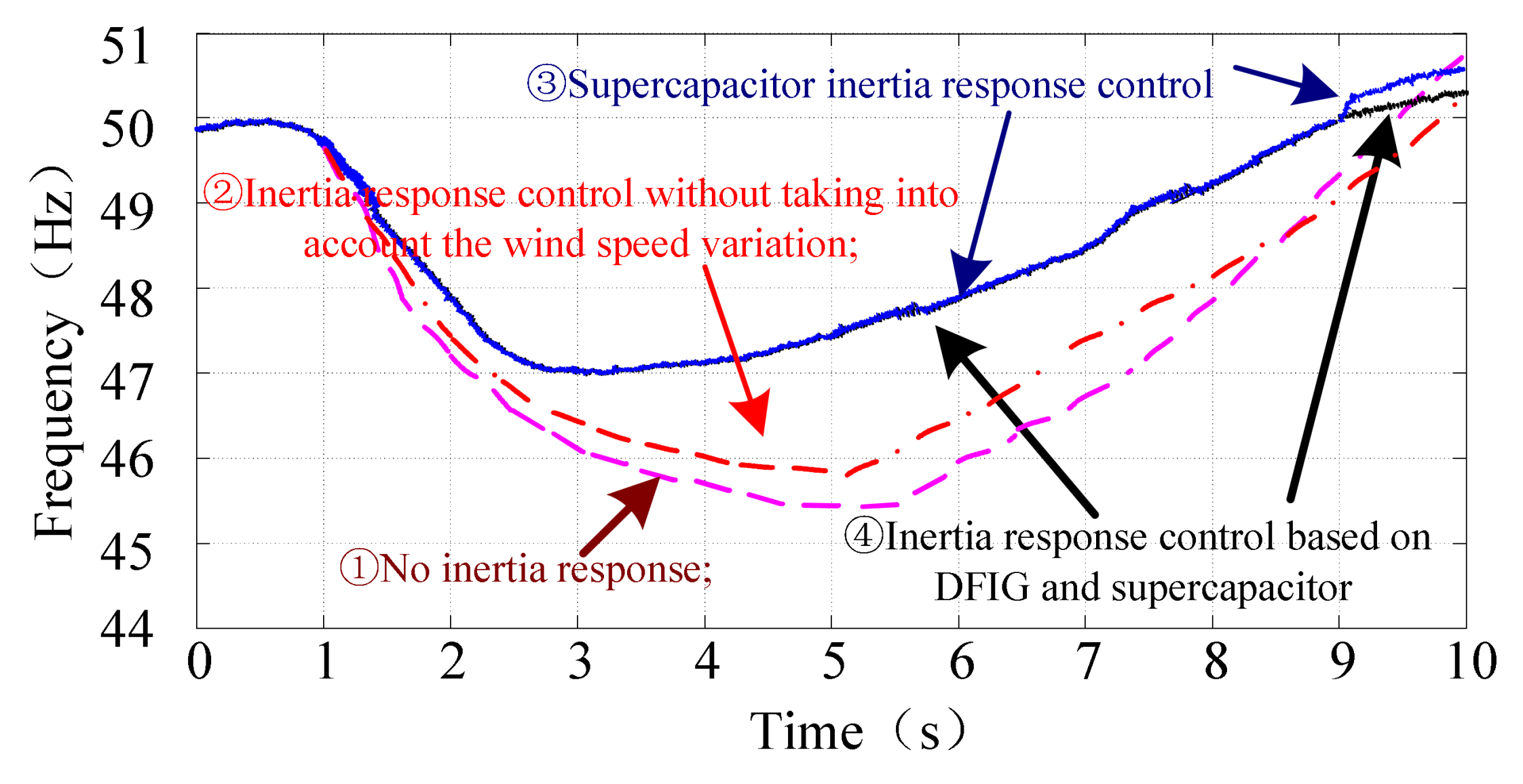
The initial simulation conditions include: the load L1 is connected in the system; the DFIG runs in MPPT mode, and the grid frequency is kept at 50 Hz. At the time of 1 s, the frequency of the power grid system falls when the shock load L2 is added. Figure 11 gives the frequency response curves of the power grid system under four different control strategies, they are: ① No inertia response; ② Inertia response control without taking into account the wind speed variation; ③ Supercapacitor inertia response control; and ④ Inertia response control based on DFIG and supercapacitor. The simulation result shows, the grid frequency falls of the control strategy ③ and control strategy ④ are lower than those of the strategy ① and ②, and the frequency recovery is more stable. That is to say, without the inertia response control adopted, or with the inertia response control but without taking the wind speed variation into account, the frequency drop amplitude of the power grid will be much larger, and much easier to be affected by the wind speed change.
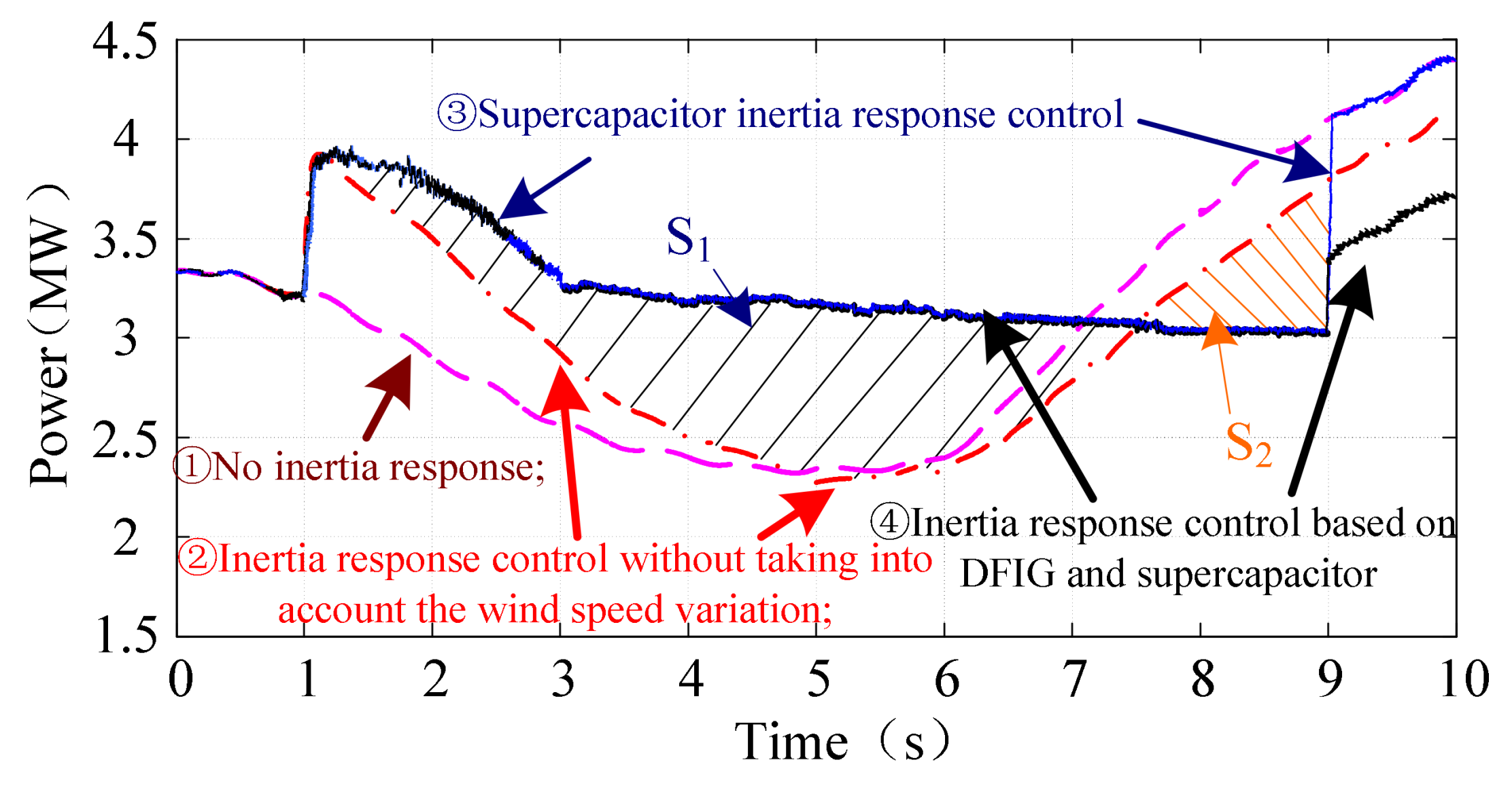
Figure 12 shows the comparison of the frequency inertia response power under different control strategies. It also suggests that, without the inertia response control adopted, or with the inertia response control but without taking the wind speed variation into account, the total output power of wind farm will be strongly affected by the wind speed change, and the output power of wind farm cannot be as stable as that of a synchronous generator. Combining the results in Figure 11, it can be concluded that the use of the supercapacitor to provide frequency inertia response power alone, or together with DFIG, the stability of the power grid can be improved by providing a controlled and stable power output similar to the synchronous generator.
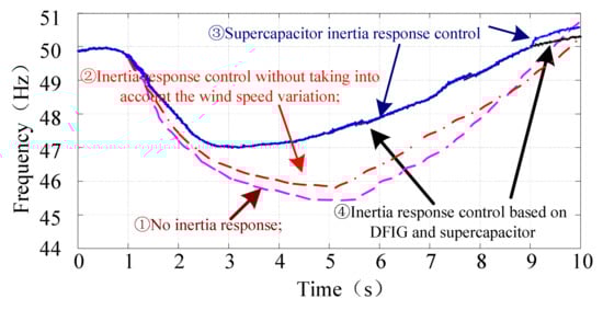
Figure 12.
Comparison of the power grid frequency responses with shock load L2 added.
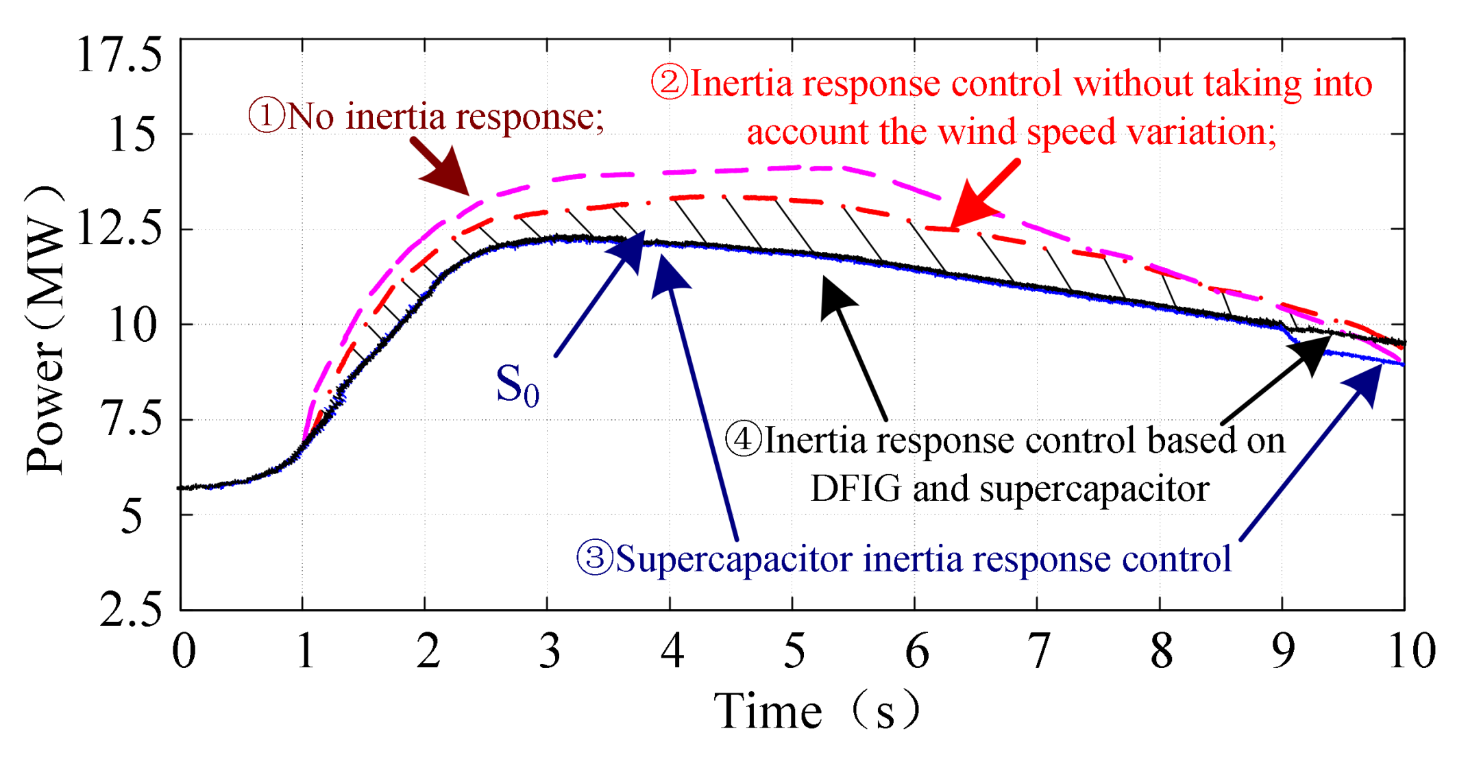
Combined with Figure 12, Figure 13 and Figure 14, it can be seen that control strategy ① is that SCESS-DFIG does not have the frequency inertia response control of power grid. After sudden loading, the frequency change rate of power grid is the largest in four kinds of control strategy, and the frequency drop amplitude is also the largest. At the same time, in order to overcome the wind speed change for SCESS-DFIG output power reduction, SG needs to continuously increase the output power. In contrast, the control strategy ② SCESS-DFIG has the inertia response control, so the change rate of the power grid is less than the control strategy ① frequency change rate, but due to the wind speed changes, SCESS-DFIG output power is reduced, which makes the SG needs to continuously increase power to maintain the power grid frequency. Control strategy ③ and control strategy ④ consider the influence of wind speed variation on the inertia response. The simulation results show that the frequency change rate of the power grid is much slower than that of the former, while the frequency drop is less. Because SCESS-DFIG itself eliminates the influence of wind speed change, the synchronous generator no longer needs to compensate for the power change of the wind turbines in the frequency inertia response of the power grid. In Figure 14, S0 is the output power of SG to eliminate the influence of wind speed fluctuation. With the further increase of wind permeability, S0 will increase with the wind speed change, which is harmful to the effective capacity of synchronous generators. Therefore, the control strategies ③ and ④ consider the wind speed change, eliminating the wind speed influence by SCESS-DFIG is very necessary.
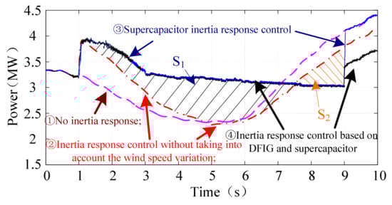
Figure 13.
Comparison of the total frequency inertia response power of wind farms under different control strategies.
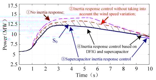
Figure 14.
Comparison of the power of SG under different control strategies.
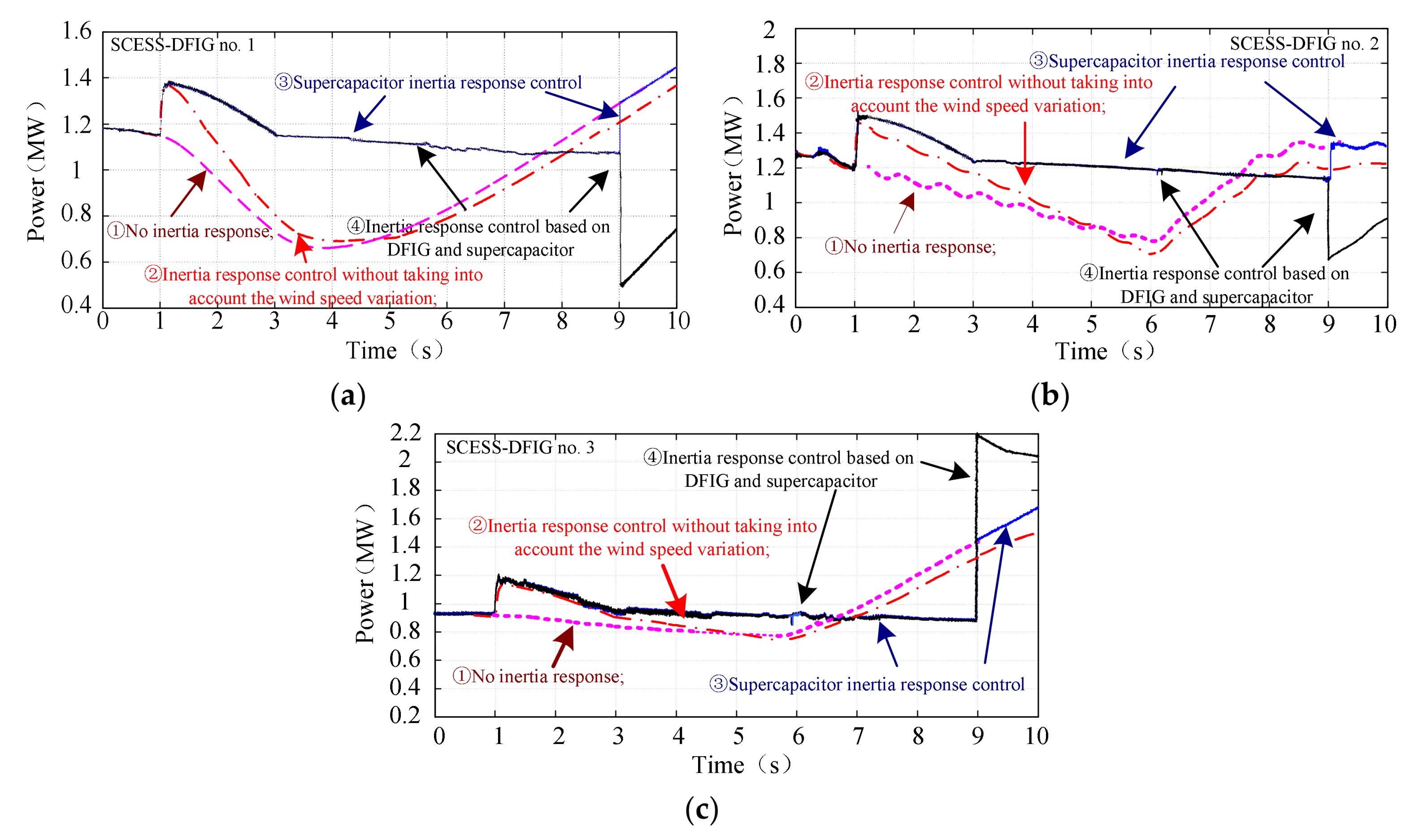
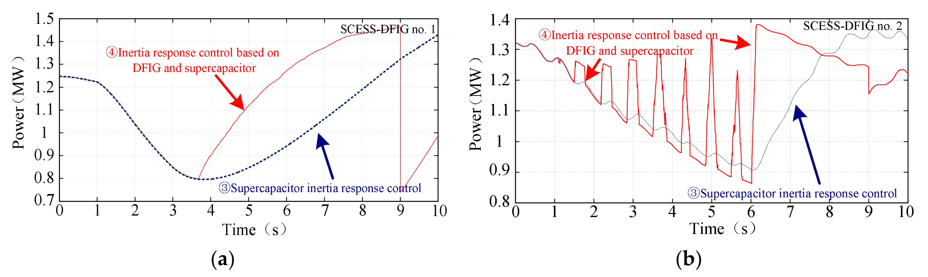
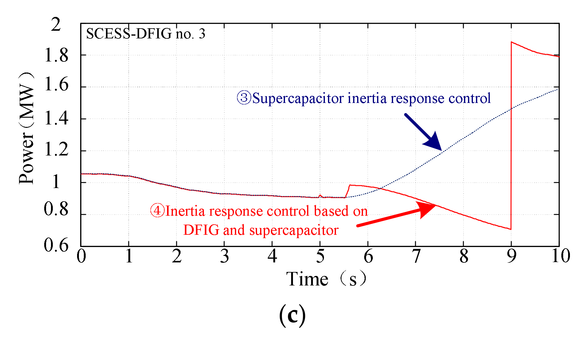
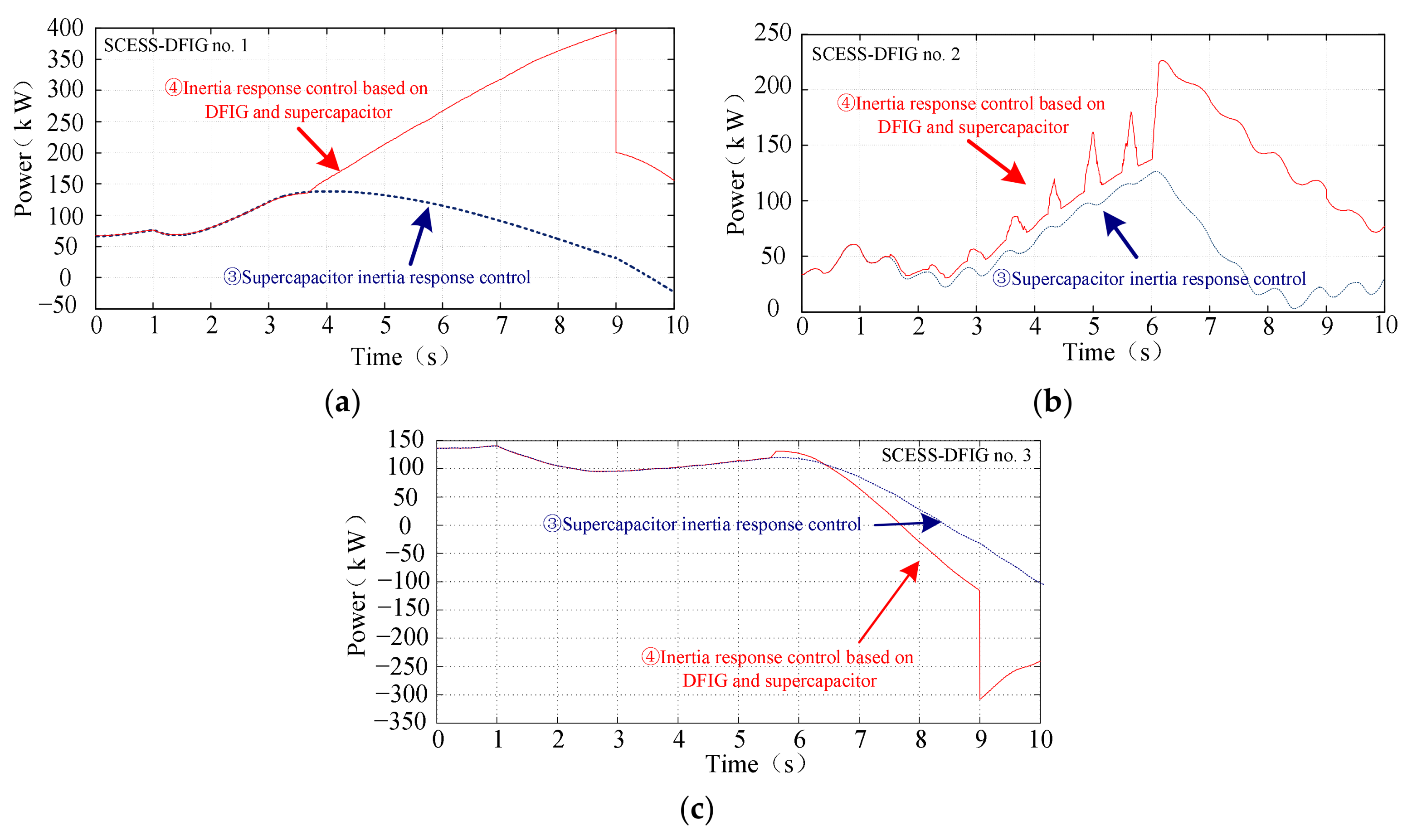
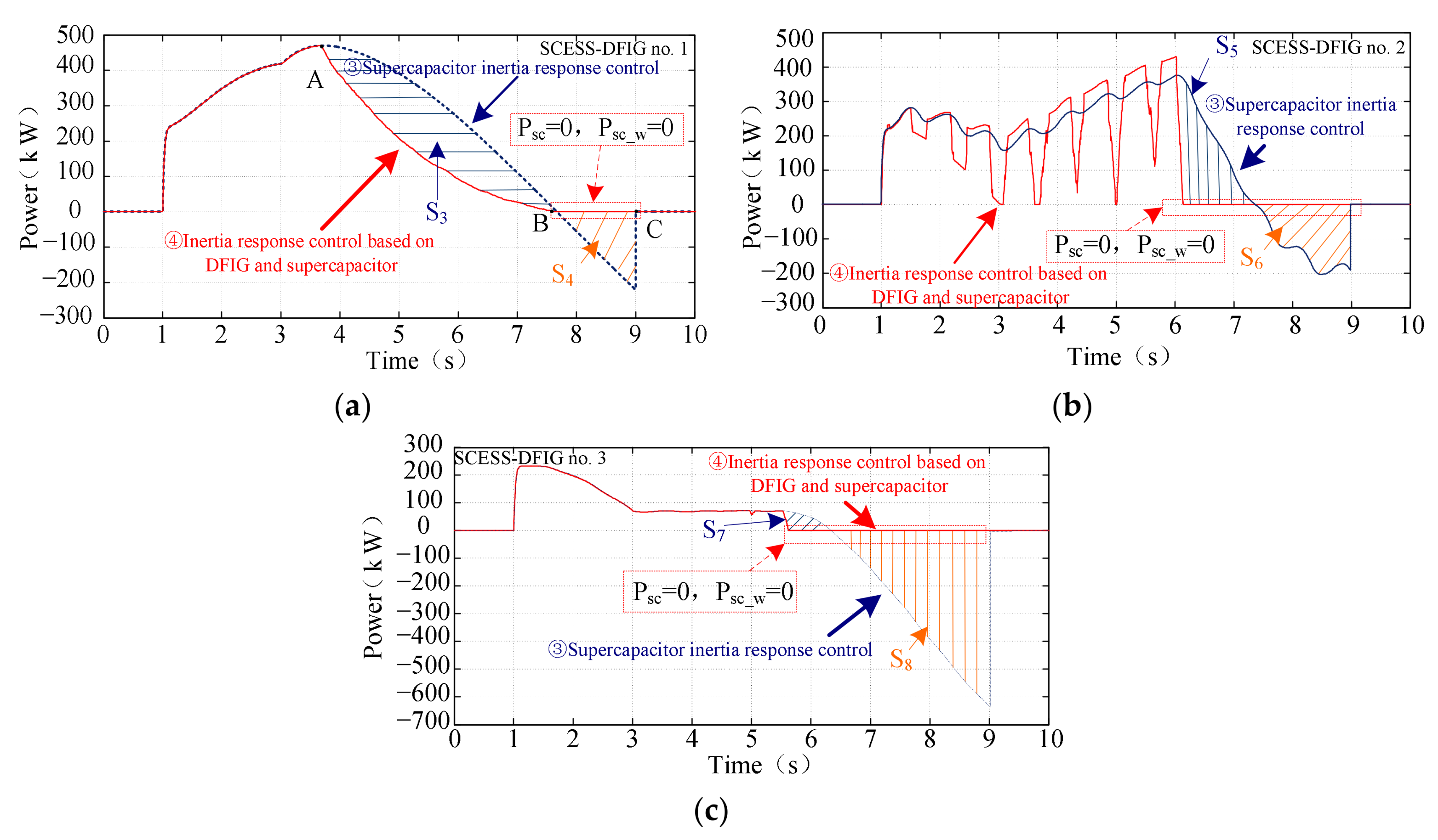
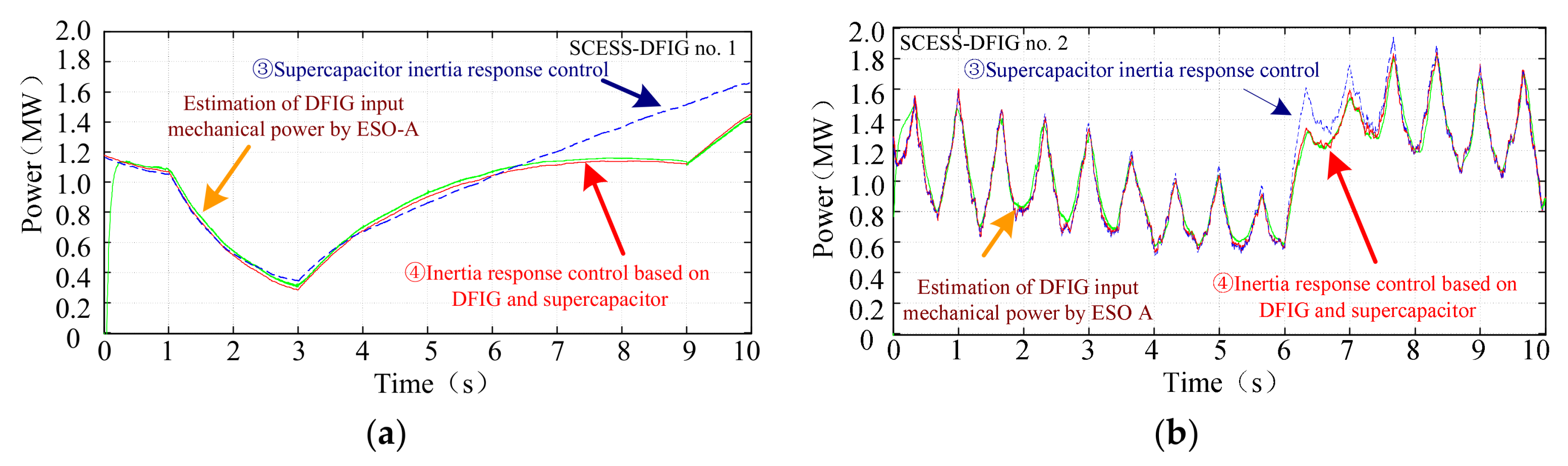
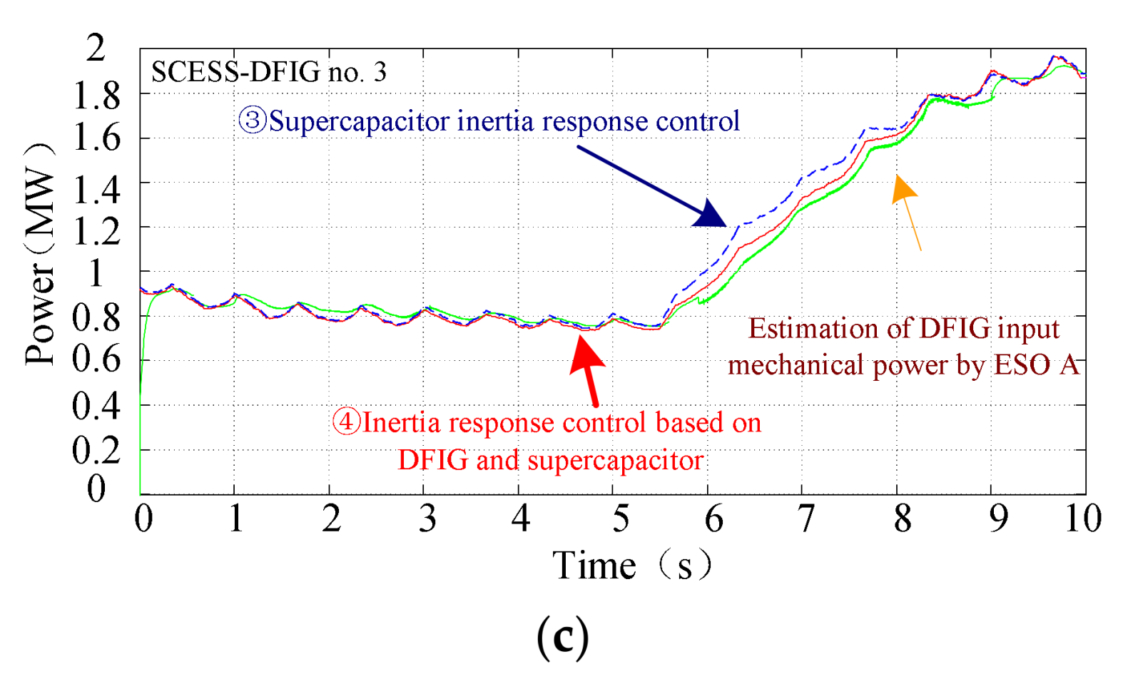
Figure 15 shows a comparison of the inertia response power of a single SCESS-DFIG with different wind speeds. The powers of the DFIG and the supercapacitor energy storage are controlled cooperatively, with the wind speed change being taken into account. The output power curve can restrain the power fluctuation caused by wind speed changes in the inertia response process, and the SCESS-DFIG can provide stable and controllable inertia response power, with MPPT control unadopted in the frequency inertia response process. It can also be noticed that, at the ending time of the inertia response—9 s—in order to restore the MPPT control, the control strategy ③ and the control strategy ④ will cause different SCESS-DFIG output electric power.
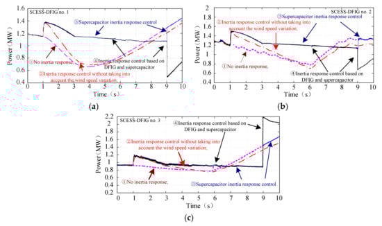
Figure 15.
Comparison of the inertia response powers of the single SCESS-DFIG under different control strategies: (a) Single inertia power response under different control strategies for SCESS-DFIG no. 1; (b) Single inertia power response under different control strategies for SCESS-DFIG no. 2; (c) Single inertia power response under different control strategies for SCESS-DFIG no. 3.
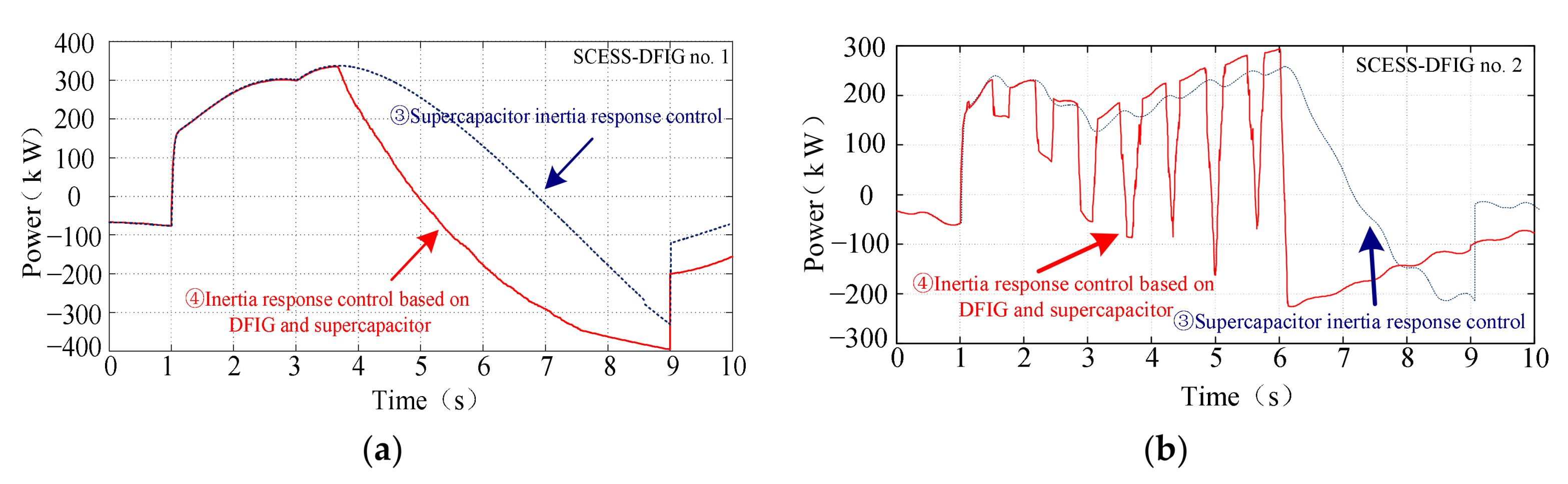
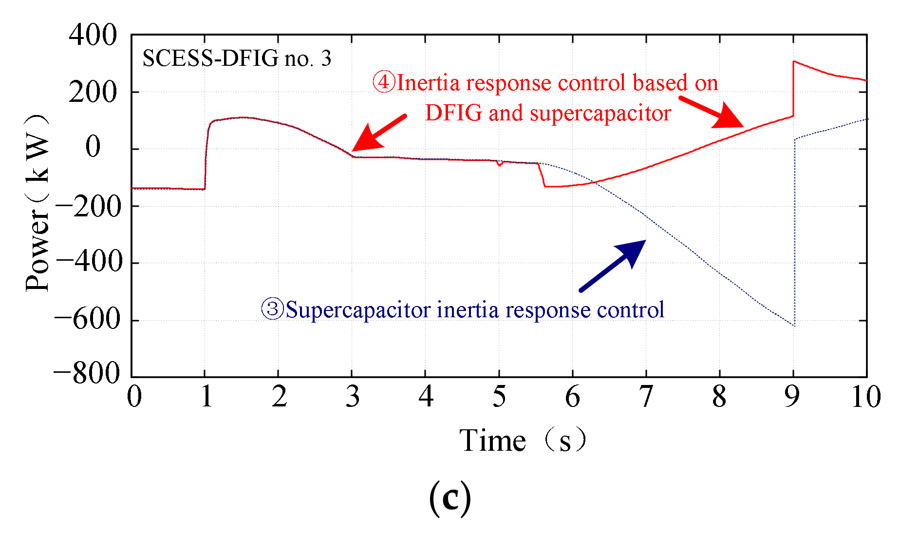
Figure 16 is comparison of DFIG output electric power Pe under different control strategies; Figure 17 is comparison of SCESS-DFIG stator output power under different control strategies; Figure 18 is comparison of output power of the single RSC under different control strategies; Figure 19 is comparison of output power of the single GSC under different control strategies
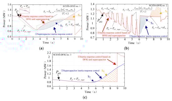
Figure 16.
Comparison of DFIG output electric power Pe under different control strategies: (a) DFIG output electric power Pe1 under different control strategies for no. 1 SCESS-DFIG; (b) DFIG output electric power Pe2 under different control strategies for no. 2 SCESS-DFIG; (c) DFIG output electric power Pe3 under different control strategies for no. 3 SCESS-DFIG.

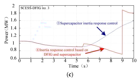
Figure 17.
Comparison of SCESS-DFIG stator output power under different control strategies: (a) No. 1 SCESS-DFIG stator output power under different control strategies; (b) No. 2 SCESS-DFIG stator output power under different control strategies; (c) No. 3 SCESS-DFIG stator output power under different control strategies for SCESS-DFIG no. 3.
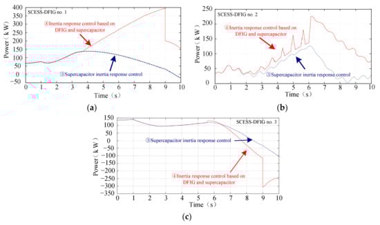
Figure 18.
Comparison of output power of the single RSC under different control strategies: (a) The RSC output power under different control strategies for no. 1 SCESS-DFIG; (b) The RSC output power under different control strategies for no. 2 SCESS-DFIG; (c) The RSC output power under different control strategies for no. 3 SCESS-DFIG.
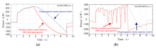
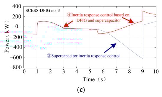
Figure 19.
Comparison of output power of the single GSC under different control strategies: (a) The GSC output power under different control strategies for no. 1 SCESS -DFIG; (b) The GSC output power under different control strategies for no. 1 SCESS-DFIG; and (c) The GSC output power under different control strategies for no. 1 SCESS-DFIG.
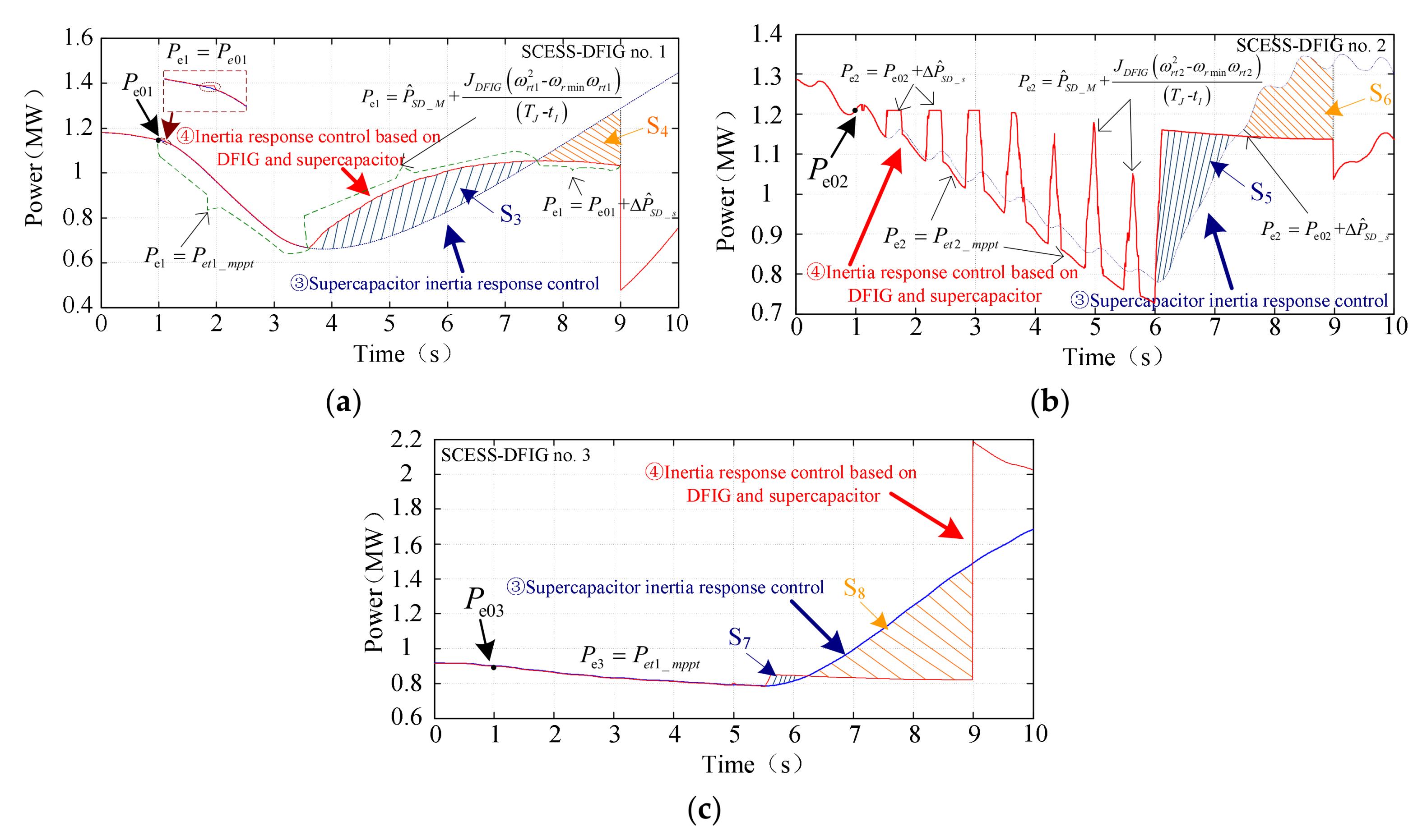
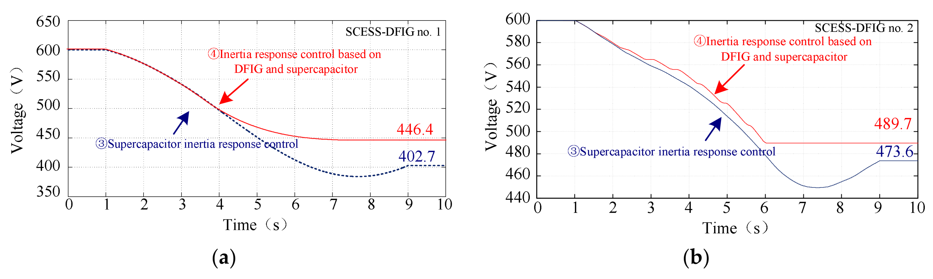
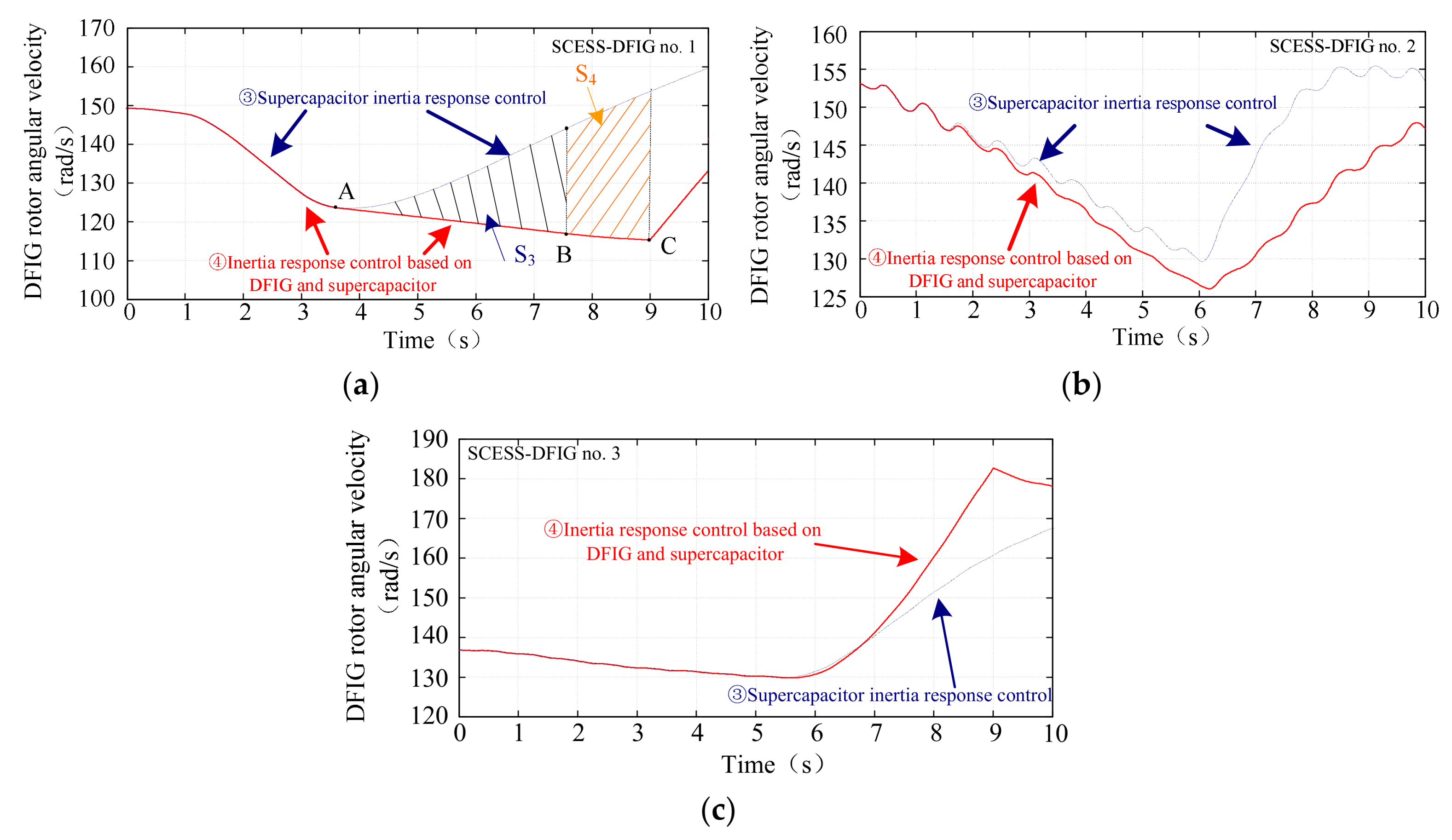
From Figure 16a, it can be observed that the estimated input mechanical power at the initial stage of frequency inertia response is less than the electronic output power Pe01. This is mainly due to the sudden drop in wind speed and wind speed changes to the power grid frequency inertia response to introduce an underdamping energy. At this point , DFIG output power is Pe1 = Pet1_mppt. Within the AB region, SCESS-DFIG applied control strategy ④ to release the rotor kinetic energy, so the DFIG output power is higher than the DFIG output power of the control strategy ③ (S3). In the BC region, with the wind speed increasing, the DFIG input mechanical power increases, Kten < 0, . As shown in It is obvious from Figure 20a that in the AB region, the supercapacitor energy storage device with control strategy ④ has a lower output power. In the BC region, the supercapacitor energy storage device does not require power regulation (Psc = 0, Psc_w = 0). As shown in Figure 21a, the supercapacitor voltage using control strategy ④ is 446.4.7 V in the end, which is greater than the value 402.7 V when the supercapacitor is the sole source to provide the frequency inertia response power. Figure 22a, due to the release of the kinetic energy of the rotor, in the AB region, the application of control strategy ④ DFIG rotor speed gradually decreased. Because of the speed protection in the control strategy ④, the rotor speed is higher than 110 rad/s.
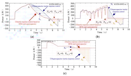
Figure 20.
Comparison of output power of supercapacitor energy storage device under different control strategies: (a) The supercapacitor energy storage device output power under different control strategies for no. 1 SCESS-DFIG; (b) The supercapacitor energy storage device output power under different control strategies for no. 2 SCESS-DFIG; (c) The supercapacitor energy storage device output power under different control strategies for no. 3 SCESS-DFIG.
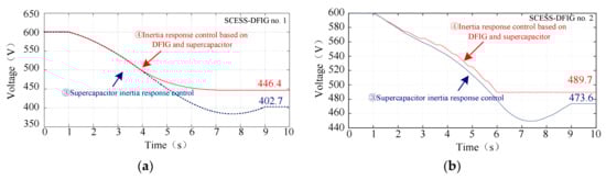
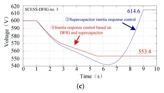
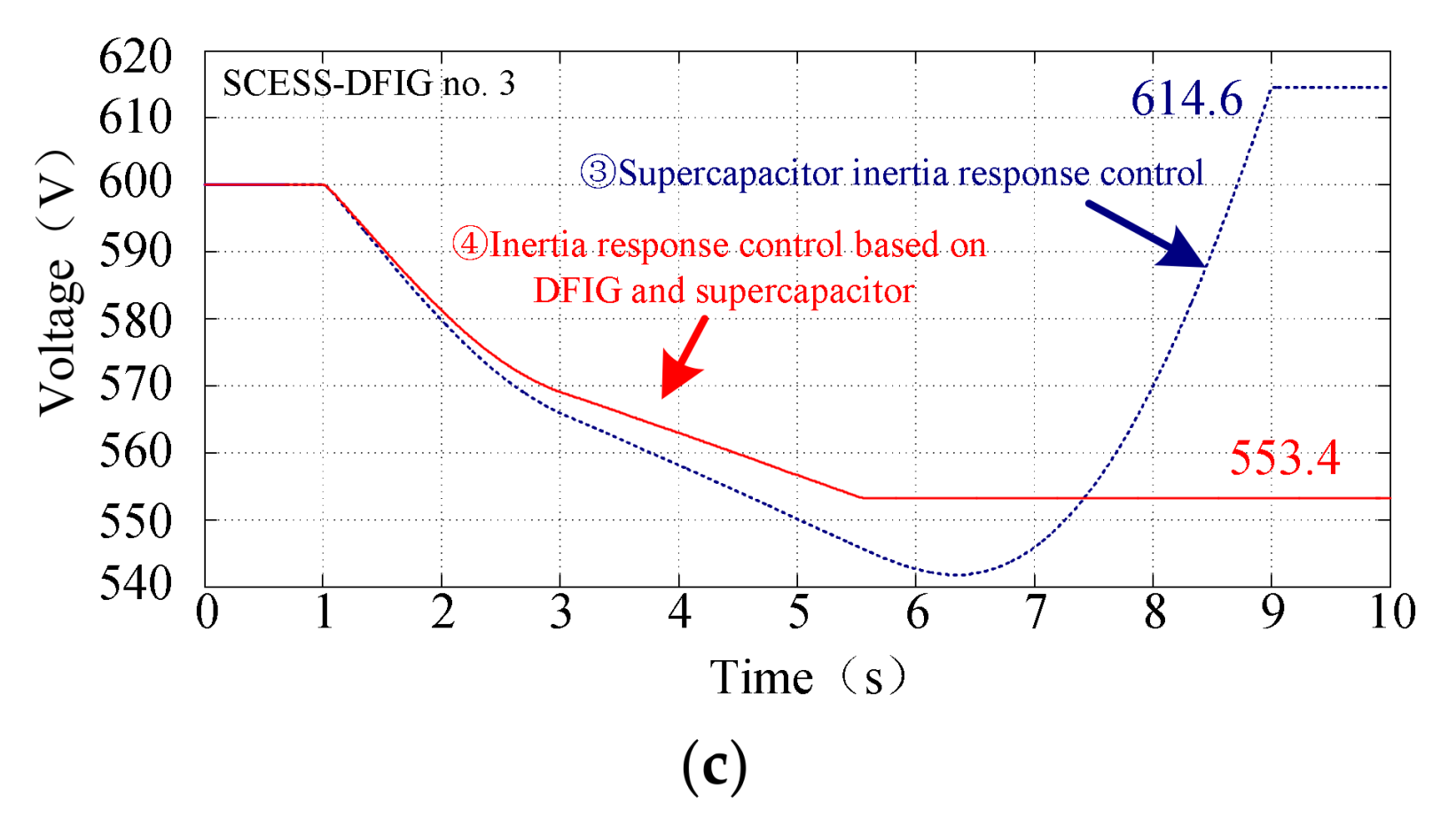
Figure 21.
Comparison of SCESS-DFIG supercapacitor voltages under different control strategies: (a) No. 1 SCESS-DFIG supercapacitor voltage under different control strategies; (b) No. 2 SCESS-DFIG supercapacitor voltage under different control strategies; (c) No. 3 SCESS-DFIG supercapacitor voltage under different control strategies.
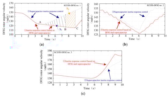
Figure 22.
Comparison of angular velocity of the SCESS-DFIG rotor under different control strategies: (a) No. 1 SCESS-DFIG angular velocity under different control strategies; (b) No. 2 SCESS-DFIG angular velocity under different control strategies; (c) No. 3 SCESS-DFIG angular velocity under different control strategies.
It is shown from Figure 16b that, in the process of power grid frequency inertia response, the kinetic energy of the rotor is released by using the control strategy ④. This provides a part of the inertia response power while stabilizing the wind speed change. Therefore, as shown in Figure 22b, the speed of DFIG decreases faster than the DIFG speed of control strategy ③. When the wind speed rises, the DFIG input mechanical power estimate is higher than the Pe02, the DFIG output power is , at this time the supercapacitor energy storage device does not have the power flow (Psc = 0, Psc_w = 0). Under control strategy ③, the DFIG is affected by wind speed, the output power is increased, the supercapacitor energy storage device in DE region output power (S5), in the EF region absorption power (S6), which resulted in additional energy loss, while increasing the demand for supercapacitance capacity.
As shown in Figure 16c, the wind speed drops, the DFIG output power is , at this time the supercapacitor energy storage device through the power control makes the SCESS-DFIG have the inertia response ability. As shown in Figure 20c, when the wind speed rises, the supercapacitor energy storage device power of control strategy ③ and control strategy ④ is compared, because SCESS-DFIG in control strategy ③ has no stratification control of wind speed change. The maximum absorption power of the supercapacitor energy storage device is 700 kW, which has reached the capacity limit of the converter. If the wind speed rises more violently, the power of the supercapacitor will be bigger, which is unfavorable to the capacity design of the DC converter and the grid side converter (GSC). SCESS-DFIG using control strategy ④ does not have such a problem.
Figure 23 is the input mechanical power comparison of SCESS-DFIG under different control strategies and the input mechanical power estimation of ESO-A. As shown in Figure 23, the ESO-A estimates the input mechanical power is effective and can be used as a control variable for the SCESS-DFIG rotor side converter.
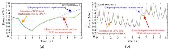
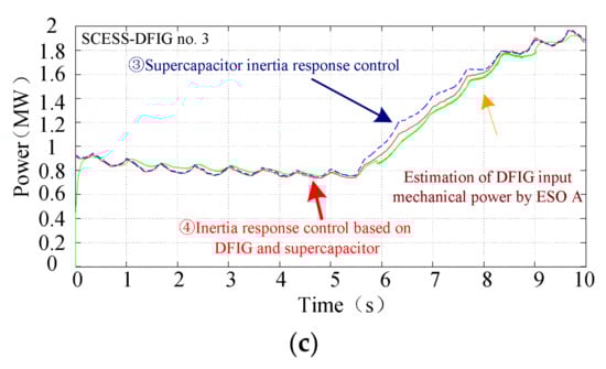
Figure 23.
The input mechanical power comparison of SCESS-DFIG under different control strategies and the input mechanical power estimation of ESO-A: (a) The input mechanical power comparison of no. 1 SCESS-DFIG under different control strategies and the input mechanical power estimation of ESO-A; (b) The input mechanical power comparison of no. 2 SCESS-DFIG under different control strategies and the input mechanical power estimation of ESO-A; (c) The input mechanical power comparison of no. 3 SCESS-DFIG under different control strategies and the input mechanical power estimation of ESO-A.
6. Conclusions
In the grid frequency inertia responses, the influence of wind speed variations on the output power of DFIG was taken into consideration, and one SCESS-DFIG topology and its principle of adjusting the output power was analyzed. The inertia time constant of SCESS-DFIG containing the influence of the wind speed variations was defined. An ESO-A was established to accurately estimate the input mechanical power of DFIG, so was an ESO-B to estimate the power for the grid frequency inertia response. The inertia response control strategy of SCESS-DFIG was designed based on the energy stratification control for wind speed change. The simulation model of SCESS-DFIG and synchronous generator was built in MATLAB/Simulink, which verified that the control strategy proposed in this paper is applicable to different variation trends of the wind speed. With the effect of wind speed changes on the output electric power of DFIG was effectively utilized, the inertia response power provided by a supercapacitor can be effectively reduced and the stability of frequency inertia response of the SCESS-DFIG power grid can be greatly improved.
Acknowledgments
This work was supported by the National Natural Science Foundation of China (grant no. 51107018), the National Natural Science Foundation of China (grant no. 51677040).
Author Contributions
Dongyang Sun conceived and designed the experiments; Dongyang Sun and Guangxin Zu performed the experiments; Dongyang Sun wrote the paper; and Lizhi Sun, Fengjiang Wu revised the paper.
Conflicts of Interest
The authors declare no conflict of interest.
Appendix A

Table A1.
The electrical parameters of SCESS-DFIG.
Table A1.
The electrical parameters of SCESS-DFIG.
| Item | Parameter | Item | Parameter |
|---|---|---|---|
| Type of generator | DFIG | Generator capacity | 2.5 MW |
| Blade radius | 42 m | Pole-pairs | 2 |
| Cp | 0.44 | Gear ratio | 1:100 |
| JDFIG | 5,000,000 kg/m2 | λopt | 6.87 |
| Supercapacitance capacity | 20 F | Supercapacitor initial voltage | 600 V |
| Rs/pu | 0.01 | Ls/pu | 0.12 |
| Rr/pu | 0.01 | Lr/pu | 0.11 |
| Lm/pu | 3.52 | TJ | 10 s |
| α1 | 0.5 | δ1 | 0.001 |
| β01 | 1000 | β02 | 10,000 |
| α2 | 0.5 | δ2 | 0.001 |
| β03 | 1000 | β04 | 20,000 |
| HSD | 5 s |
Table A2.
Parameters of synchronous generator SG.
Table A2.
Parameters of synchronous generator SG.
| Item | Parameter | Item | Parameter |
|---|---|---|---|
| Xd/pu | 2 | X’d/pu | 0.35 |
| X′′d/pu | 0.252 | Xq/pu | 2.19 |
| X′′q/pu | 0.243 | X1 | 0.117 |
| T′d/pu | 8 | T′′d/pu | 0.068 |
| X′′q/pu | 0.9 | Hs | 4.8 s |
Appendix B
PD Control parameters: Kp = 10, Kd = 5.
Fuzzy logic control parameters:
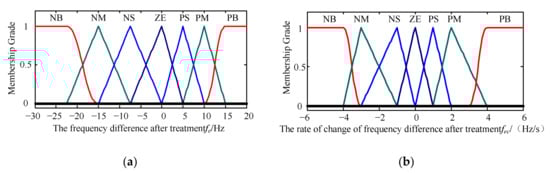
Figure A1.
Membership function of input variable: (a) Frequency deviation membership function; (b) Frequency deviation change rate membership function.
Figure A1.
Membership function of input variable: (a) Frequency deviation membership function; (b) Frequency deviation change rate membership function.
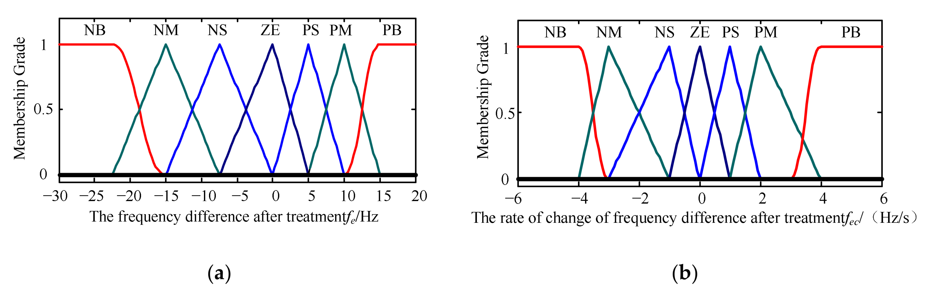
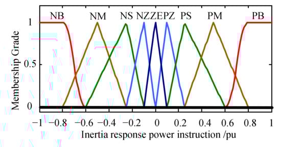
Figure A2.
Membership function of output variable.
Figure A2.
Membership function of output variable.
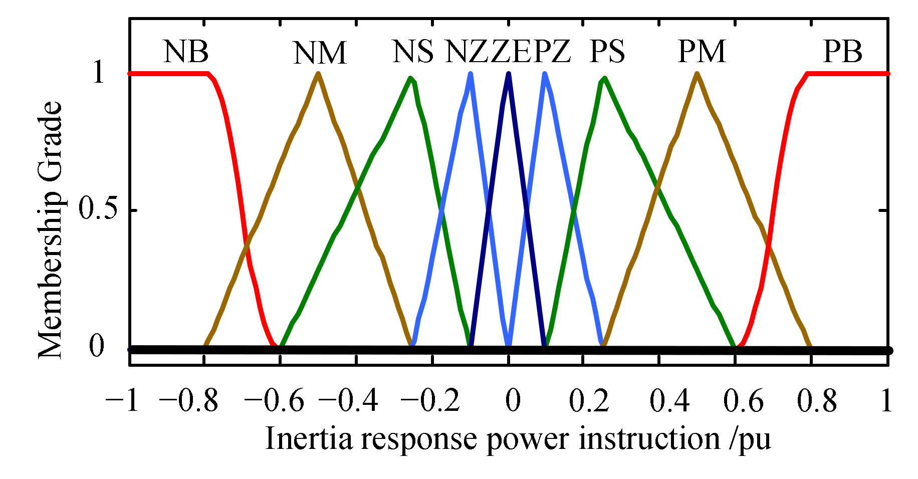
Table A3.
Fuzzy logic rules for controller.
Table A3.
Fuzzy logic rules for controller.
| Inertia Response Power Control U | Frequency Deviation fe | ||||||
|---|---|---|---|---|---|---|---|
| Frequency deviation rate fec | NB | NM | NS | ZE | PS | PM | PB |
| NB | PB | PB | PB | PB | PZ | ZE | NS |
| NM | PB | PB | PB | PM | ZE | NZ | NM |
| NS | PB | PB | PM | PZ | NZ | NS | NB |
| ZE | PB | PB | PM | ZE | NS | NM | NB |
| PS | PB | PM | PS | ZE | NM | NB | NB |
| PM | PM | PM | PS | NS | NB | NB | NB |
| PB | PM | PS | PZ | NM | NB | NB | NB |
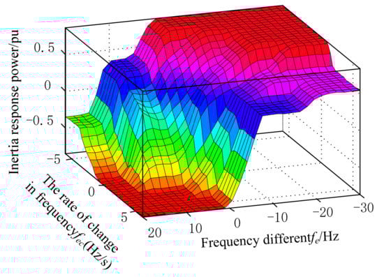
Figure A3.
Result of fuzzy logic inference.
Figure A3.
Result of fuzzy logic inference.

References
- Shu, Y.; Zhang, Z.; Guo, J. Study on Key Factors and Solution of Renewable Energy Accommodation. Proc. CSEE 2017, 1–9. [Google Scholar] [CrossRef]
- Yuan, X. Overview of problems in large scale wind integrations. J. Mod. Power Syst. Clean Energy 2013, 1, 22–25. [Google Scholar] [CrossRef]
- Liu, J.; Yao, W.; Wen, J. Prospect of Technology for Large-Scale Wind Farm Participating Into Power Grid Frequency Regulation. Power Syst. Technol. 2014, 38, 638–646. [Google Scholar]
- Morren, J.; de Haan, S.W.H.; Kling, W.L. Wind turbines emulating inertia and supporting primary frequency control. IEEE Trans. Power Syst. 2006, 21, 433–434. [Google Scholar] [CrossRef]
- Li, H.; Zhang, X.; Wang, Y. Virtual inertia control of DFIG-based wind turbine based on the optimal power tracking. Proc. CSEE 2012, 32, 32–39. [Google Scholar]
- Ramtharan, G.; Ekanayake, J.; Jenkins, N. Frequency support from doubly fed induction generator wind turbines. IET Trans. Renew. Power Gener. 2007, 1, 3–9. [Google Scholar] [CrossRef]
- Vidyanandan, K.V.; Nilanjan, S. Primary frequency regulation by deloaded wind turbines using variable droop. IEEE Trans. Power Syst. 2013, 28, 837–846. [Google Scholar] [CrossRef]
- Li, L.; Ye, L. Coordinated control of frequency and rotational speed for direct drive permanent magnet synchronous generator wind turbine at variable wind speeds. Autom. Electr. Power Syst. 2011, 35, 27–31. [Google Scholar]
- Teninge, A.; Jecu, C.; Roye, D. Contribution to frequency control through wind turbine inertial energy storage. IET Trans. Renew. Power Gener. 2009, 3, 358–370. [Google Scholar] [CrossRef]
- Cao, J.; Wang, H.; Qiu, J. Frequency control Strategy of variable-speed constant-frequency doubly-fed induction generator wind turbine. Autom. Electr. Power Syst. 2009, 33, 78–82. [Google Scholar]
- De Almeida, R.G.; Peas, L.J.A. Participation of doubly fed induction wind generators in system frequency regulation. IEEE Trans. Power Syst. 2007, 22, 944–950. [Google Scholar] [CrossRef]
- Zhang, Z.S.; Sun, Y.Z.; Lin, J. Coordinated frequency regulation by doubly-fed induction generator based wind power plants. IET Trans. Renew. Power Gener. 2012, 6, 38–47. [Google Scholar] [CrossRef]
- Ding, L.; Yin, S.; Wang, T. Integrated frequency control strategy of DFIGs based on virtual inertia and over speed control. Power Syst. Technol. 2015, 39, 2385–2391. [Google Scholar]
- Fu, Y.; Wang, Y.; Zhang, X. Analysis and Integrated Control of Inertia and Primary Frequency Regulation for Variable Speed Wind Turbines. Proc. CSEE 2014, 34, 4706–4716. [Google Scholar]
- Liu, J.; Yao, W.; Wen, J. A wind farm virtual inertia compensation strategy based on energy storage system. Proc. CSEE 2015, 35, 1596–1605. [Google Scholar]
- Xiong, L.; Li, Y.; Zhu, Y.; Yang, P.; Xu, Z. Coordinated Control Schemes of Supercapacitor and Kinetic Energy of DFIG for System Frequency Support. Energies 2018, 11, 103. [Google Scholar] [CrossRef]
- Liu, Z.; Liu, F.; Mei, S. Application of extended state observer in wind turbines speed recovery after inertia response control. Proc. CSEE 2016, 36, 1207–1217. [Google Scholar]
- Wang, B.; Xu, Y.; Shen, Z. Current Control of Grid-Connected Inverter with LCL Filter Based on Extended-State Observer Estimations Using Single Sensor and Achieving Improved Robust Observation Dynamics. IEEE Trans. Ind. Electron. 2017, 64, 5428–5439. [Google Scholar] [CrossRef]
- Ma, X.; Chen, Y.; Su, J. Speed Estimation Method for Brushless Doubly-fed Machine Stand-alone Generation System Based on Model Reference Adaptivity Application of extended state observer in wind turbines speed recovery after inertia response control. Proc. CSEE 2017, 37, 5171–5180. [Google Scholar]
- Han, J. Active Disturbance Rejection Control Technique: The Technique for Estimating and Compensating the Uncertainties; National Defence Industry Press: Beijing, China, 2008. [Google Scholar]
- Han, J. The “Extended State Observer” of a class of uncertain systems. Control Des. 1995, 10, 85–88. [Google Scholar]
- Chang, X.Y.; Li, Y.L.; Zhang, W.Y.; Wang, N.; Xue, W. Active disturbance rejection control for a flywheel energy storage system. IEEE Trans. Ind. Electron. 2015, 62, 991–1001. [Google Scholar] [CrossRef]
- Zhong, Q.; Zhang, Y.; Yang, J.; Wu, J. Non-linear auto-disturbance rejection control of parallel active power filters. IET Control Theory Appl. 2009, 3, 907–916. [Google Scholar] [CrossRef]


© 2018 by the authors. Licensee MDPI, Basel, Switzerland. This article is an open access article distributed under the terms and conditions of the Creative Commons Attribution (CC BY) license (http://creativecommons.org/licenses/by/4.0/).