Abstract
This paper describes the evolution of the thermal network and its applications for making simplified thermal models of buildings by means of thermal resistances (R) and capacitances (C). In the literature, there are several modelling schemes for buildings. Here, we investigate the advantages, disadvantages, and improvements of thermal networks. The thermal network method has been used in different studies for calculating indoor air temperature and heating load, estimating model parameters, and studying building interactions with heating and cooling systems. This review paper conducts an investigation into the application, system identification, and structure of thermal networks compared to other tools. Within the framework of the thermal network method, we conclude with some new proposals for research in this field to expand the idea of the thermal network to other engineering and energy management fields.
1. Introduction
Buildings are one of the main sectors for energy reduction efforts in EU countries. They consume around 40% of total used energy and are responsible for more than 35% of carbon emissions [1]. Hence, building and district energy management and optimisation problems have been identified as being an interesting and challenging topic for engineers. Such problems have been receiving much attention due to the importance of energetic or economic themes. For instance, energy engineers are primarily interested in: the main energy sources in various historical times, district energy systems and how they operate, available energy sources according to the time and region, design considerations for residential and industrial zones, and reducing greenhouse gas emissions and their environmental impacts. Furthermore, economic feasibility, performance analysis, and the role of energy policies [2] represent other fields of research.
Until now, energy engineers have put a lot of effort into energy production potential, modelling, and optimisation, although district energy system management and greenhouse gases are still crucial issues [3]. According to the literature, energy efficiency at the district level depends on the performance of the heating and cooling systems, the energy consumption, the energy production, and the energy losses in distribution systems.
Engineers have developed various methods to quantify and optimise the used and produced energy on large and small scales (district or building scale) [4,5]. The common modelling approaches are categorised as deterministic energy models, stochastic energy models, and artificial neural networks. In deterministic energy models, the key parameters influencing the heat demand must be identified [6]. On the other hand, stochastic modelling is mainly used for forecasting and has not been used significantly for nonlinear problems [7]. Finally, artificial neural networks are used when many parameters are included in the model [3], and the model is derived from available datasets [7]. It is necessary to develop interactions between different modelling methods, as this favours the production of simple, robust, and verified models. This objective can be facilitated by means of machine learning techniques to make models and computers capable of learning from datasets and patterns without being explicitly programmed [8]. Several studies have identified that a data-driven model with a combination of deterministic and stochastic models is reliable enough to express envelope properties and forecast indoor conditions and the heating load [9,10,11,12]. Experimental results demonstrate that the hybrid model exhibits a better performance compared with the other techniques. In fact, all the predictors constructed by means of the energy-consuming patterns have a more reliable performance than those designed only by the construction data [13].
Another type of categorisation of modelling techniques is steady-state and dynamic models, which can be used in both forward and inverse approaches. The degree-days method is applicable to calculating the amount of energy that a heating system uses from one day/week/month/year to the next. Although this method can provide accurate results for calculating the peak and average loads for sizing the system, it is not very interesting for modelling dynamic indoor conditions, occupancy behaviour, and building interactions studies [6,14]. Furthermore, sophisticated technologies for energy metering and environmental monitoring, in cooperation with communication and networking technologies, can be key features of future smart buildings and grids [15,16], where transient responses of the thermal performance of buildings play a vital role instead of steady state solutions.
After a description about different building energy performance techniques and some of the available tools, this paper focuses on the thermal network method as an alternative approach, which has shown its capability to simulate and forecast the thermal load of a building in different problems. In addition, with an interest in data-driven models for various applications in building energy management such as thermal load prediction [17], electricity consumption models [18], and local energy production [19], the thermal network method provides results that are as accurate as neural networks, in addition to maintaining the real interpretation of specified parameters. In this context, despite other review papers that describe the thermal network as an option along with other tools for building energy performance, the main contribution of this review paper is to cover the main applications of thermal networks for building energy assessment. It includes studying the functionality of the thermal network method for inverse modelling and system identification problems and concentrating on the importance of the structure of thermal networks for different applications.
The rest of this paper is organised as follows: Section 2 studies different steady state and dynamic modelling methods, categorising available models into three different groups, named as forward, inverse, and hybrid approaches. Section 3 looks at the different applications of the thermal networks method to assess energy problems in buildings and it concludes with five main categories for building energy management problems and the application of the thermal network method for each type of problem. Section 4 considers inverse modelling and data-driven models with the available system identification approach for parametric models and the thermal network method. Section 5 details how different thermal network structures are developed for simulating internal mass effects, multi-zone buildings, and appliances. Section 6 investigates the functionality of thermal networks in comparison to available software and tools, in addition to investigating how effectively engineers used the outcomes of the available software and tools to train various thermal networks and parametric models. Finally, Section 7 presents the conclusion and suggests new research proposals to expand the application of the thermal network method for energy problems of buildings.
2. Building Energy Performance Simulation
Evidently, the consumed energy required to keep a zone in proper comfort and health conditions depends on various factors [20], such as indoor temperature, humidity, chemical contents, ventilation rate, surface temperatures, and PPD level (predicted percentage of dissatisfied). Indoor comfort opens new areas of research for the development of various controllers for HVAC (heat, ventilation, and air conditioning) systems, electric power, illumination, and new technologies, such as smart meters, occupancy detectors, sensor technologies, and building to grid characterisation [21].
Generally, between 50% and 70% of the total used energy in a building is consumed to provide the thermal comfort [22]. Thus, developing a suitable control system based on a thermal model of buildings that can manage preferences for indoor air quality in the most optimised situation has been studied by many researchers [23,24]. As previously mentioned, the steady-state and dynamic models are the two main approaches for determining the annual energy consumption of buildings. The stationary heat balance equation is a well-known approach for making steady-state models. This method provides a summary of the outside temperature’s effects on the building’s constant indoor air temperature. While, in some specific cases, the heat loss coefficient and the efficiency of the HVAC system are affected by the outside temperature, the steady-state model is considered for different temperature intervals and time periods: this is called the Bin method [25].
Steady-state models provide good results for determining the maximum required loads by assuming that the internal temperature of the building does not change throughout the whole year. If the aim is to optimise the annual energy consumption, a variable indoor temperature considered in dynamic models will be of greater use for designers. Some preliminary work for transient thermal models was carried out in 1967 by introducing the response factor method [25,26] and the periodic heat flow model to determine the “total equivalent temperature differential” for a building. The dynamic approach generally includes the thermal network method, modal analysis, differential equations, autoregressive moving average modelling (ARMA), Fourier series, and transfer functions. Available techniques for calculating the energy consumption for buildings and districts are shown in Figure 1.
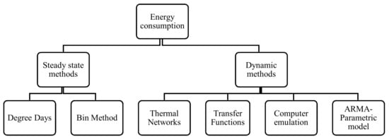
Figure 1.
Commonly used methods for building thermal performance assessment.
The numerical calculations give the possibility to dynamic models to calculate very accurate results when discretised time steps are used. Nowadays, different types of software are available to determine the energy consumption in buildings by means of steady-state or dynamic models [27]. A study from K.U. Leuven (Belgium) calls into question the margin of error for steady-state and dynamic simulation methods for a low-energy building in a social housing company. It has been shown that the EPW (Flemish energy performance regulation–semi-steady state model) calculates the total energy demand, with a small excess in accuracy compared to software using dynamic models, such as TRNSYS and ESP-r [28].
The presented models in Figure 1 can be categorised into forward, inverse, or hybrid approaches. A forward approach (Degree days, ASHRAE conduction transfer function) is a time-consuming approach in terms of preparing the initial information for a model. It is used when detailed information about the building is known and is also called white box modelling. Difficulties in preparing detailed information for modelling buildings as a white box problem push engineers to search for alternative solutions using simplified models. These new techniques are less comprehensive, in physical terms, but the modelling and mathematical formulations are much simpler than white box models. In fact, data-driven models are extracted from specific datasets. They are also called black box models (ARMA model) and use inverse modelling. A more practical solution can rely on a hybrid model. The hybrid modelling technique is a combination of forward and inverse methods together, also called grey box modelling.
Neural network models, linear parametric models (Transfer functions), and thermal network methods are described in the literature as possible simplified models of buildings [29]. Among the available simplified models, the thermal network method is considered as a grey box model with an interesting approach for providing fast and accurate results through a simple representation of the different heat transfer features of a building. In the next chapter, the simplified models, especially the thermal network method, are of concern and the main applications of this method in different kinds of literature are described.
3. Applications of the Thermal Network Method
The thermal network method provides a very simple method for moving from a steady-state domain to a transient domain. Thanks to the effort of researchers, the thermal network method has become one of the most reliable ways to make accurate building models. In this section, we will present a literature review based on some of the available literature from the 1990s to 2016. We will try to clarify the advantages, disadvantages, and the evolution of this method during these years to introduce new subjects of research into this topic. In general, the thermal network method has been applied in different research areas such as analysing different wall structures, building and heating system interactions, system identification, thermal mass and storage, solar radiation, and multi-zone models.
Some preliminary work for developing a thermal network to calculate transient heat transfer in a plane wall was carried out in the 1980s. Hassid [30] investigated the first 2R1C model for calculating the energy savings in passive solar buildings. He described his model with three quantities: the total thermal conductance (U), the responses of the elements to temperature, and solar radiation changes which originate inside (L) or outside (M) the building within a 24-h period. He used the 2R1C structure, as shown in Figure 2a, to calculate L and M for different buildings. His model is based on the minimum and maximum indoor temperature during the day and night. He claimed this model could be extended to study storage walls and two-zone effects by doubling the equations. Two years later, Seems [31] used a more complicated model with 3R2C, shown in Figure 2b, to determine transient heat transfer in a plane wall. These studies represent the early attempts to motivate building designers to use a thermal network analysis procedure. At that time, representing all the complicated heat transfer phenomena inside the model (ex: multi-layered elements or high mass wall and ground connections) was the main problem.
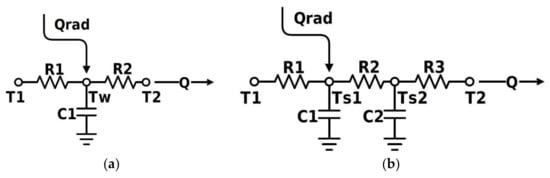
Figure 2.
The early thermal network models for plane wall structures. (a) 2R1C model with Tw showing the wall temperature; (b) 3R2C model with Ts1 and Ts2 showing the wall surface temperatures.
The early studies come to the conclusion that thermal mass calculation is a challenging issue and several studies have been conducted on this subject. In 1991, Mathews [32] introduced a new method to calculate the effective heat storage of a building by relating the massive layer capacitance to the resistance of each layer. In his analysis, β factor affects the thermal capacitance of each layer of a building. In fact, β is the ratio of the resistance of each layer to the total resistance of a multi-layer wall (from the outdoor temperature to the indoor temperature) for exterior layers. On the other hand, for interior elements, the β depends on the ratio of half the resistance of a layer and the resistance of this layer up to the indoor surface. Mathews verified the accuracy of his model with the experimental results from 62 different buildings. Mathews’ model [32] is able to predict accurate indoor air temperature for unoccupied office blocks, shops, schools, residential buildings, low mass well-insulated structures in contact with the ground, and low and high mass poorly insulated structures.
Mathews’ method also presented a new idea for determining other parameters in simplified thermal networks. One year later, in 1992, Lombard [33] developed a new method based on the time constant of the building, to consider the variations of the parameters with time. This assumption gives a better description for studying natural and forced ventilation in thermal networks. In addition, he showed that the time step of 1 h is adequate for most types of structures (stable solution), but for very light structures, the maximum time step must be 15 min. He proposed the method for a first-order model and concluded with a possible extension to higher order models.
When inverse methods become an alternative approach for determining the parameters of thermal networks, researchers figured out that identified parameters in thermal networks differ from the thermal properties of structures. In fact, the lumped capacitance assumption, used in thermal networks, accumulates the effects of many elements into a few parameters that can affect the physical interpretation of thermal networks [34]. Although the inverse modelling approach might not estimate accurate parameters, it could provide better adjustment between adapted models and measurements compared to the deterministic approaches that were already being used.
Progress in numerical analysis and computer performance during the past decade has helped engineers to solve more complicated equations and thus more complex models. The 3R2C model for simulating transient heat transfer in plane walls had already been used [31], but its application in the making models of buildings, and even more complicated structures, has become easier. Furthermore, more complicated structures with 3R4C for a plane wall, or considering a 2R1C for each layer of a multi-layer wall, could help to make more complex models, and even RC ladders [35].
In 2002, Fraisse [36] made a comparison between different thermal branches, one with a 3R4C wall branch, and others with simpler thermal networks using 2R1C and 3R2C. The aim of his study was to use thermal networks for convective and longwave exchanges with a linear model. He proved that a 3R2C model provides results as accurate as the 3R4C model for a plane wall structure. Therefore, it should not be necessary to use a very detailed model for further applications of thermal networks. In addition to this achievement, Fraisse [36] made one of the early designs for studying the interaction of a thermal network of a building with the electric and hydraulic heating floor. He also managed to get very accurate outputs for a coupled model. However, he did not give a detailed explanation of the identified parameters and their physical interpretation. Moreover, the interaction between the heating system and building model was also studied by Romaní [37]. He summarised the main characteristics of a thermally activated building system (TABS) with the implementation of the thermal network method and control strategies for the thermal model of buildings.
Thermal networks have also been used to investigate new methods to optimise envelope structures and minimise energy losses in buildings. For instance, Gonzalez [38] introduced a novel method for parameter estimation of a 3R2C model, called the dominant layer method. This method represents the massive layer of a wall with one resistance and one capacitance, and the other resistances and capacitances represent other wall layers. He showed that this new method provides even more accurate results than those from transfer functions. In 2009, Sambou [39] optimised a wall construction by introducing the thermal network impedances in the frequency domain. He determined the effective wall capacitance and wall construction to estimate the optimal thickness and effective capacitance of the massive layer. At first, he optimised four different types of structures and concluded that thermal inertia plays an important role in summer thermal comfort and in winter energy demands. He concluded that there is a direct relationship between insulation layer thickness and the thermal capacitance of the massive layer for heat loss reduction. In another work on simulating building structure by means of RC networks, Cheng [40] determined the building impedance and time lag. He tried to achieve the most optimised structure for a wall, and finally, concluded that a seven-layer wall with the massive layer in between the insulation layers presents the smallest energy losses.
The importance of solar radiation in energy assessments of buildings is undeniable and researchers develop different methods to implement this crucial factor by means of thermal networks. Ogunsola [41] did not consider radiation on walls directly in his thermal network and he decided to use solar-air temperature in a 3R2C structure. However, a deeper study on solar radiation effects on the required heating/cooling load was conducted by Yan [42]. He presented a method to consider the radiative heat flux on the inner surface of external envelopes to improve the accuracy of thermal networks. He showed that simplifying the zone configuration might make a small error in load calculation that is not significant.
The internal mass effect, containing internal walls and furniture, is another challenging issue. The consideration of furniture thermal mass for large buildings is essential, but very difficult to estimate. Ogunsola [43] proposed a simple model made of a 3R2C branch to show the wall and roof effects and a 2R2C branch to show the internal mass effect, as well as specifying a branch with one resistance to show massless windows. He tested this model for three different types of the building structure (light, medium, and heavy structured walls), and he included uncertainty for input information, such as solar radiation and outside temperature. In these cases, the identified model for a light structure building generates larger errors compared to other types of buildings.
Another application of thermal networks for energy assessments in buildings was done by Ginestet [44], who intended to make a calculation device for architects in order to determine the suitability of the initial sketch, from the energy consumption point of view. In his tool, a 2R1C model is identified for a multi-layer wall with a reflective Newton algorithm. In addition, he tried to optimise the thermal insulation, the heat capacity of the wall, and the building’s heating load.
Eco-design requirements for energy efficiency lead to the importance of defining European regions with common climatic characteristics [45]. The capability of thermal networks to calculate heating and cooling loads in different climates was also studied by De Rosa [46]. He used a simple RC network in different countries to study the effects of different environmental conditions on the proposed model. He defined degree-days as a climate parameter of each place, which reinforced the functionality of his model in different European countries. He highlighted the fact that the linear relationship between heating load demand and heating degree-days (number of days that a building needs heating load) in European countries is due to the large values for heating degree-days (HDD > 800). On the other hand, he defined the modified cooling degree-days (CDD) to develop another linear correlation between cooling load demand and CDD.
Lastly, a complete review of different building modelling methods demonstrates that grey box models, especially thermal networks, are effective models for making a sophisticated building energy management system [47]. Thermal networks are customised for use with either white or grey box models. In addition to studies trying to explore suitable modelling features of thermal networks [48], some researchers consider other aspects for developing new control situations of smart buildings [37], longwave radiation [49], green walls effects [14], and multi-zone models [50]. In addition, the thermal network method has been used to study the application of phase change materials (PCM) in building envelope components for thermal storage [51,52] with assuming non-linear capacitances. Ventilated cavity walls and concrete slabs [53,54] can also be considered by developing thermal networks with parallel branches. Furthermore, various glazing systems are usually studied as a set of resistances and the thermal masses are omitted in proposed thermal networks [55]. Overall, we can categorise different applications of thermal networks to structure analysis, system identification of thermal networks, indoor conditions and energy consumption, solar radiation and heat gains, and finally building interactions, as shown in Table 1.

Table 1.
Thermal network applications in different problems.
4. Inverse Modelling and System Identification
System identification facilitates the application of thermal networks, though it brings other complexities when interpreting the physical descriptions of thermal networks. One of the first applications of the system identification approach for determining the parameters of an RC model for a school building was done in 1990 by Penman [60]. He used the least square technique to determine different resistances and capacitances in his 3R2C model. He studied the reliability of parameters and the accuracy of identified parameters in the thermal network for integration with BEMS (Building Energy Management System). He showed three out of his five parameters could be identified accurately, though there were large differences between identified values for indoor capacitance and external resistance. Finally, he concluded that the deviations between the identified model and experimental data might be constrained to the constant adjustment of unidentified parameters.
At that time, identifying five parameters for BEMS was cumbersome, so Coley [61] used least square error algorithms with upper and lower limits for parameters to identify the same model as Penman with shorter periods of time. According to his observations, initial values generated some oscillations in the model’s outputs. The model’s parameters reached their almost steady values after the 500th time step, and the identified parameters are in good accordance with Penman’s work. These studies were the first to integrate building thermal network models with control systems by means of online parameter calculation [61].
Immediately afterwards, Dewson [62] worked with the same RC network as Penman and Coley to elaborate the details of the identification problem using the RMS (Root Mean Square) technique. He explained the uncertainties in identification algorithms related to the existence of multiple local minima, the extreme sensitivity of some parameters compared to others, and poor convergence, etc. He specified three different tests for each parameter, and showed small deviations of parameters from their actual values, despite the good “fit” of the measured temperatures with the model’s output. Dewson presented his work with a second-order model for a one-zone building, and he questioned the capability of the method to simulate multi-zone buildings and the identification of physically-related parameters.
Since 2000, the system identification approach has been accepted as a powerful procedure for identifying the model parameters of unknown systems, especially in the field of energy performance in buildings. The available algorithms [63,64], informative conditions [65,66,67], and other aspects of the system identification method are studied in different books and papers.
A system identification problem is usually bonded to some uncertainties in the identified parameters, the model’s reliability, multiple local minima, the information matrix, and experiment design, etc. DYNASTEE [68] is a pioneering group who collect and study such effects on the identification problem in buildings. They have tried to improve and strengthen the basis of system identification techniques in building modelling by holding competitions and workshops for more than 10 years. Androutsopoulos [69] collected and compared the data for 10 years of competitions to present the progress of system identification in building energy management. He concluded that to identify thermal networks, regarding the best and worst results, the identified value for thermal resistance R was calculated almost equally by all competitors. However, the thermal capacitances had very scattered values.
System identification is also a strong tool for the application of parametric models (transfer functions). Parametric models have been used for energy assessments in buildings which are mainly based on statistical analysis [48]. Unfortunately, parametric models and thermal networks have not formed a large part of the literature until the last decade, because of the lack of experimental data and slow computers for data processing purposes. Since 2008, most of the works on thermal modelling of buildings have concentrated on system identification for parametric models and thermal networks. Wu [70] showed that parametric models can simulate the indoor air temperature for university offices with a very high accuracy for short and long periods. This dataset contains 109 days of data for 374 rooms and spaces in a university building. At the same time, thermal networks provide a more elegant solution, since they determine accurate results while also maintaining the physical characteristics of buildings.
Nowadays, system identification toolboxes and packages are available for most programming languages, such as MATLAB [71], R [72], Python, Labview, and JModelica [73], etc. These toolboxes and packages contain many functions for linear and nonlinear identification. They have very powerful functions to describe a physical model, with transfer functions, or state space models. In addition to black box models, some languages provide specific tools for grey box modelling, such as the MATLAB system identification toolbox, E4 toolbox [74], the CTSM package in R [75], and LORD (LOgical R-Determination), which is specifically for thermal network identification [76]. These tools facilitate the implementation of the thermal network method for making inverse models.
Jiménez [10,77] used MATLAB’s system identification toolbox to make LTI (Linear Time Invariant) parametric models of a building. She made a correspondence between simple RC network components with ARMAX (Autoregressive moving average model with exogenous inputs) model coefficients. Therefore, each coefficient in the identified model was a combination of a set of parameters from the thermal network. She calculated the indoor temperature, the difference between the indoor and outdoor temperatures, U-values (thermal transmittance), and the heating load as the outputs of the model. In addition, her determined U-values presented very low errors compared to the experimental results. In her work, she used the toolbox to determine the U-value for only one wall and did not apply it to the whole building. Jiménez used the system identification toolbox to check the data, select the order and the structure of the parametric model, and for the identification of parameters.
The system identification approach increased the interest in studying certain aspects, such as internal mass and appliances effects by means of thermal networks, in more depth. The first studies of appliance effects in contact with thermal networks started by adding a new branch to a building model. Park [78,79] introduced a 1R1C branch to consider appliances in a building, as shown in Figure 3a. She determined the thermal network parameters as a function of identified parameters in different parametric models (ARX (Autoregressive exogenous), ARMAX, BJ (Box–Jenkins), and OE (Output error)). She concluded that for a second order building model, the ARX model provides the most accurate results according to her experimental data. In another work, Wang [80] used a genetic algorithm to determine the parameters of the model by means of data collected from an office building over a period of two weeks. This model contains all the effective capacitances of the envelope, including the walls and roof. In addition, he considered the internal mass (internal walls, furniture, and appliances) by means of a 2R2C branch (3R2C+2R2C), as represented in Figure 3b. He was able to simulate indoor temperature with a high accuracy, though he did not provide any explanations about the accuracy of identified parameters for the internal mass branch.
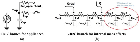
Figure 3.
The branches added to study. (a) appliances; and (b) internal mass effects.
As mentioned earlier in this paper, a good model can be developed by integrating different techniques at the same time, and the thermal network method is able to be integrated easily with other methods. The application of the thermal network method in conjunction with transfer functions was investigated by Xu and Wang [81]. In their work, they simulated the same building in [80], but this time, they used a transfer function to model some parts of the building for which enough detailed information was available, such as the structure’s materials. For other parts, without sufficient information, they used a 2R2C branch and estimated the parameters of that branch using a genetic algorithm. The RC branch was connected to transfer functions and operated the same way as if there were no transfer functions, and as if the RC thermal networks modelled the whole building. Usually, the coefficients of the transfer functions are easily available, or they can be easily calculated using the physical properties of the building’s envelope [25]. The optimal parameters for the 2R2C, in this case, were similar to their values in another work [80], which used a complete thermal network (3R2C+2R2C).
The progress in the thermal network method and the ease of making a thermal model of buildings in forward or inverse modelling problems has motivated researchers to develop new mathematical methods for finding buildings’ thermal properties. Peng [82] introduced a new harmonic method to solve thermo-electrical circuit equations, which he called TEAM (Thermoelectricity Analogy Method). For this purpose, he proposed new equations to calculate the decay rates and time lag of a thermal network by means of electrical analogy and could then determine the temperatures of each node accurately. He showed that the proposed method is as accurate as the Laplace method, and it is easier to apply than harmonic methods.
Furthermore, the application of parametric models to simulate and forecast the humidity ratio has been investigated by Mustafaraj [83]. He used linear parametric models to make a temperature model and a relative humidity model for a building. He used BJ, ARX, ARMAX, and OE models to identify the thermal behaviour of an office. He showed that a second order model is accurate enough for temperature simulations because all the equations for temperature are linear, while the relative humidity is a nonlinear phenomenon. Therefore, a seventh order model was needed. Overall, we can compare the different modelling techniques and the general conclusions about the system identification approach as it is represented in Table 2.
Table 2.
Overall description of inverse modelling in buildings.
5. The Structure of Thermal Networks
The previous sections have focused more on the application and development of thermal networks rather than the complexities and limitations of working with them. A controversial problem in the thermal network method is the number of capacitances and resistances. If the model does not have enough capacitances and resistances, then it may fail to provide accurate results. On the other hand, identification algorithms need lots of time to identify the parameters in very complicated models with a large number of resistances and capacitances. Moreover, the complicated models might be accurate for one building but might fail to simulate another building with an insufficient dataset. In fact, categorising thermal network methods as simplified models seems to be somewhat deceptive. The truth is that these models can become complex very easily. If the purpose of the model is to show multi-layer structures, different branches of the walls, roof, windows, ground, longwave radiations, etc., then the number of parameters increases exponentially.
For instance, Deng [84] used 37 capacitances to indicate a detailed thermal RC network for a four-room office. On this ground, we can argue that solving a thermal network with 37 capacitances for a building is a very complicated and time-consuming problem. He used model reduction techniques, such as aggregation of state, to reduce the number of capacitances to one capacitance for each room. Deng’s findings lend support to the claim that the model reduction technique does not have a major effect on parameters. In fact, any new component in the reduced model will be a summation of previous components obtained with a higher order model.
Kramer [85] studied various RC models by increasing the number of resistances and capacitances to find the appropriate model for a building. Finally, he concluded that a model with three capacitances can provide accurate results and that a more complicated model is unnecessary. As reported by Kramer, increasing the number of capacitances to more than three did not have a large effect on the model’s accuracy. Unfortunately, he did not clarify the accuracy and physical interpretation of the identified parameters. He just used the term of effective parameters, rather than apparent parameters, to explain the differences between the real values and the identified ones.
Reynders [86] studied the quality of grey box models and also identified parameters for different thermal networks. He used first to fifth order RC models and trained the models with five different datasets. He used a CTSMR package [75] (stochastic modelling) implemented in statistical computing language (R) [87] to identify the capacitances and resistances of his models. He also used the IDEAS library in Modelica to provide training data. He concluded that from a first-order model to a fifth order model, a large number of buildings can be modelled accurately, whether the building is well insulated or not. In the case of identified parameters, he identified the total conductance (UA) of the building accurately for third order, and more complex, models. However, the identified parameters for walls and indoor air capacitances were not as accurate as UA values. In another work, the multi-zone problem was studied by repeating a similar thermal network for each zone and adding a 2R1C branch to consider the adjacent walls. It was shown that repeating a 4R3C thermal network (seven parameters for a room) to model a three-zone problem can explode to a 16R11C (27 parameters) thermal network [50]. What one can conclude from the literature is that not every thermal network is able to represent all the thermal features of a problem, and researchers try to develop their thermal networks according to the most important modes of the system.
6. Software and Tools
Until now, the thermal network methods have been detailed through their applications, the use of inverse modelling and system identification, and their different structures. Besides, a large part of the literature in the field of building energy assessment describes the vast potential of the available software and tools. Furthermore, the accuracy and functionality of the thermal network method and available tools have been compared in numerous works. Thus, it seems interesting to introduce the main advantages and disadvantages of these available software and tools in comparison with the thermal network method. In addition, a comparison between the outcomes of the available software and tools and the thermal network method provides a better vision on how the thermal network method remains a competitive approach.
In the literature, parametric models and the thermal network method tend to be used for energy assessments in buildings. Still, the main concern when using the thermal network method is to yield a reliable approach to determine and predict the heating/cooling load for energy optimisation purposes. EPISCOPE (Energy Performance Indicator Tracking Schemes for the Continuous Optimisation of Refurbishment Processes in European Housing Stocks) and TABULA (Typology Approach for Building Stock Energy Assessment) are two good examples of European projects which provide rich databases to determine energy consumption for different buildings in different countries, based on the degree-days method [88]. Considering that the degree-days method deals with the steady-state solution of the problem, its results are not very suitable for dynamic solutions and control purposes. On the other hand, available software can provide quite accurate transient results, in addition to a detailed description of the envelope and connections with heating systems and electrical networks.
According to a survey among more than 800 architects and engineers, there is a large difference of interests between two groups to use available tools for buildings energy assessment [27]. The results confirm that engineers are more interested in the accuracy of their models, as well as the validation and calibration of their models, while architects devote more attention to creating sustainable models, as is presented in Figure 4. However, another survey illustrates variabilities in accredited building energy performance compliance demonstration software [89]. The uncertainties related to available software and tools to generate post-accredited models are the main shortcoming for most of the available tools. It has also been shown that one user can make a variation in simulation results up to 40% among different tools. Moreover, the lack of the effective establishment of energy setting parameters is known as the obstacle in the process of building performance data setup in some of the available tools [90]. Nevertheless, available software and tools play a vital role in building performance simulation. The application of simulation tools for artificial lighting [91], passive cooling of buildings [56], and correlation of building energy use intensities, estimated by various building performance simulation programs [92], are strong features in the building performance simulation and tools.
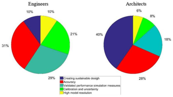
Figure 4.
Ranking criteria concerning tools accuracy.
Generally, the available tools for making dynamic thermal models of buildings are mainly based on deterministic models. Therefore, the thermal load forecast for buildings is calculated on the basis of physical principles. These equations can vary from very crude estimates of the thermal properties up to detailed comprehensive building models [93]. A comparison of 20 different available software packages and tools shows that multi-disciplinary tools, such as “CitySim”, “TRNSYS”, “EnergyPlus”, “ESP-r”, “IDA ICE”, and “Modelica” libraries, are capable of covering many or all of the areas of interest [94]. However, calculations which are completely based on the physics of the building are usually applied to single buildings, and they have not been significantly used in district simulations [95], and studies demonstrate the difficulties of ensuring that valid and consistent compliance outcomes are generated [24].
The screening process for detailed and simplified models of buildings tool selection among presented materials by Allegrini et al. [94] is shown in Figure 5. Here, building energy management problems are categorised into five groups. The detailed, simple, and not implemented models are scored with 2, 1, and 0 values. According to Figure 5, TRNSYS and ESP-r contain detailed models for each energy management problem category. TRNSYS [96] is used to simulate thermal and electrical energy systems for a single zone or multi-zone problem. Thermal modelling (solar thermal collectors, heat pumps, fuel cells), electrical modelling (photovoltaics, cogeneration, wind turbines), district heating networks, and detailed building energy simulation are the main strengths of this tool. On the other hand, “ESP-r” [97] is as strong as TRNSYS; however, it does not provide detailed models for long-wave radiation. Also, both pieces of software do not model transportation and embodied energy. “EnergyPlus” [98] is another powerful tool for building and district simulation, and is a free and open source software. Although it covers almost the same criteria as TRNSYS and ESP-r, it does not provide detailed models for photovoltaics, wind power, and thermal storage.
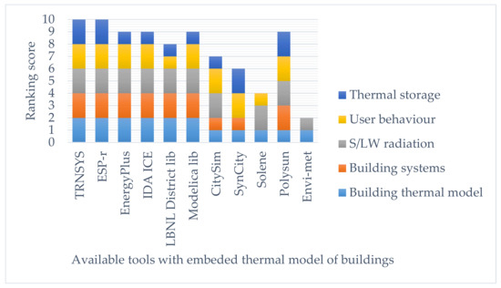
Figure 5.
Data screening of available tools with embedded thermal model of buildings.
The Modelica Buildings Library is another free open-source library with dynamic simulation models for building energy and control systems. The library contains models for HVAC systems, controls, heat transfer between rooms and the outside, multi-zone airflow (including natural ventilation and contaminant transport), single-zone computational fluid dynamics coupled to heat transfer and HVAC systems, and electrical DC and AC systems (with two- or three-phase), that can be balanced and unbalanced. The primary use of the library is for flexible and fast modelling of building energy and control systems to accelerate innovation leading to cost-effective, very low energy systems for new and existing buildings. In contrast to tools which use detailed models of buildings, CitySim [99] uses the thermal network method for single and multi-zone simulation. Other tools such as Polysun and Solene use the stationary heat balance equation.
The development in different software packages has been another challenging point for the application of the thermal network method. New software with very detailed libraries could change the applicability of the thermal network method. These developed pieces of software and tools can provide accurate results by considering very detailed information about a building’s geometry and geographical situation [100] in order to calculate and optimise consumed energy in buildings [101,102]. Indeed, some studies have been done to compare the accuracy of available software and tools with the thermal network method. For instance, in 2005, Nielsen [103] studied the effects of windows on indoor conditions in simplified models. He focused on the relationships between solar energy transmittance, incidence angles, and shadings. He determined parameters for internal and external construction properties according to EN ISO 13786 [104] and showed that a simple thermal network could provide results which are as accurate as Bsim (developed by the Danish Building and Urban Research team), even if it used comparatively little input information.
A complete study to identify the thermal network of a building for temperature and load calculation was done by Ogunsola in 2015 [41,43]. At first, he trained his model by means of two different datasets (summer and winter). Then, he compared the outputs of his thermal network to the outputs of EnergyPlus. Finally, he reached the conclusion that the identified thermal network provides results that are more accurate, and that it is adaptable for different building structures, which makes it suitable for the building energy management system (BEMS). Indeed, the trained RC network parameters are estimated according to the outcomes of buildings (indoor temperature and heating/cooling load), while available software and tools make the model by considering the physical properties of the problem, and they include more physical phenomena in their simulation schemes. Therefore, if detailed output information such as envelope temperature, convective and radiative heat transfer rates, and wind effects are not of interest, and if sufficient measurements of a building or district are available, such as the indoor conditions of each zone, heating load, and weather conditions, then thermal networks can offer quite accurate estimations with limited parameters.
Due to the lack of experimental data for different problems, researchers use the outcomes of available software and tools for specific building simulations to train different thermal network structures [86,101,105]. The consequence of this collaboration is to investigate various thermal network models in accordance with different buildings, different properties, and different geographical situations, in order to achieve the best configuration for simplified models. A comparison between the functionality of the commercial software and detailed models compared to the thermal network approach is given in Table 3. It can be concluded that not every model is able to simulate all desired phenomena. Thus, designers should choose their modelling technique according to the individual problem specifications. If the model is supposed to deal with detailed output information about the envelope, flow features, and thermal properties of different elements, then this requires a detailed CFD, or simpler model, available with the presented software and tools in Figure 5. Nevertheless, if the general output information, such as heating load and indoor temperature, is sufficient, then thermal network and parametric models are of more interest.
Table 3.
A comparison between available software and tools and the thermal network method.
In conclusion, many works [60,61,62] depict that model identification and thermal networks can easily determine accurate results and physical properties of a building in order to develop a sophisticated building energy management system.
7. Conclusions
In this paper, a literature review of the thermal network method has been provided to cover different research studies which have mainly been done between 1990 and 2016. The main idea was to highlight the progress and capability of this method to make dynamic thermal models of buildings. The paper investigates this topic concentrating on available models, applications, system identification, structure, and available software and tools.
Overall, it can be concluded that although the thermal network method has not been used to represent nonlinear phenomena such as relative humidity, it still provides quite accurate models for simulating indoor temperature and load demands. In addition, among the available simplified models, they can also represent the physics of the building and boundary conditions which give a clear idea about the system compared to neural networks. The capability of the thermal network method to simulate and predict the thermal performance of buildings with a high accuracy and limited information makes it a distinguished method compared to detailed modelling methods. The disadvantage of this method is that it can become complex very easily. If clever assumptions are not taken into account, then a large number of resistances and capacitances will be required to make a building simulation. Furthermore, the application of this method, in terms of control systems, is not often considered, and some developments are still needed to couple thermal networks to building energy management systems.
With the vast application of thermal networks in various research problems, it seems that the thermal network method can be an option for future research concerning energy assessments in buildings and districts. Additionally, despite the vast application of the thermal network method, it seems that most of the presented works in this domain lack adequate data analysis techniques. Most of the developed algorithms for system identification facilitate the calculation process to minimise the error between model outputs and measurements. However, the error minimisation is the first step for system identification and engineers must implement it post analysis (residual analysis, correlation analysis, etc.) to validate the accuracy and uniqueness of their model. Thus, it is really important to consider problems and uncertainties, such as informative dataset preparation, local minima convergence, and the parameter correlations, which can occur through the implementation of the system identification methods. By means of data-preparation and model analysis techniques, engineers can make a presumption about the number of required parameters, the identifiable and non-identifiable structures, the adequate number of variables, and the adequate number of observations to generate a unique identification problem.
In addition to those investigations on mathematical issues, future works need to be done to establish the thermal network method for building energy assessments: one of the interesting topics of research would be the simultaneous analysis of the HVAC systems with building thermal models. The unified modelling approach for different kinds of heating and cooling systems, along with the thermal network model of buildings (when available), would lead to the development of an efficient building energy management system.
The application of the thermal network method to study non-linear and stochastic phenomena can be other subjects for research. These studies can be conducted through the conjunction of wind speed and humidity ratio models with the thermal network method. In addition, considering time-dependent parameters (resistances and capacitances) in the structure of thermal networks can also represent an interesting area for further research. Another encouraging topic is the application of thermal networks for large-scale modelling (district simulation), studying interactions between buildings, coupling district thermal networks to central heating and cooling systems, occupancy behaviour, and optimising energy consumption at the district level. In sum, the prospect of being able to implement the thermal network method for a net-zero energy district serves as a continuous incentive for future research.
Acknowledgments
This work has received funding from the European Commission under the RE-SIZED (Research Excellence for Solutions and Implementation of Net Zero Energy City Districts) project, as part of Grant Agreement No. 621408.
Author Contributions
Ali Bagheri wrote the main manuscript; Véronique Feldheim supervised the research; Christos S. Ioakimidis and Véronique Feldheim performed the final revision for paper submission.
Conflicts of Interest
The authors declare no conflict of interest.
References
- European Commision. EU Energy in Figures, Statistical Pocketbook 2016; Publications Office of the European Union: Brussels, Belgium, 2016; ISBN 978-9-27-958248-6. [Google Scholar]
- Lake, A.; Rezaie, B.; Beyerlein, S. Review of district heating and cooling systems for a sustainable future. Renew. Sustain. Energy Rev. 2017, 67, 417–425. [Google Scholar] [CrossRef]
- Olsthoorn, D.; Haghighat, F.; Mirzaei, P.A. Integration of storage and renewable energy into district heating systems: A review of modelling and optimization. Sol. Energy 2016, 136, 49–64. [Google Scholar] [CrossRef]
- Evins, R. A review of computational optimisation methods applied to sustainable building design. Renew. Sustain. Energy Rev. 2013, 22, 230–245. [Google Scholar] [CrossRef]
- Swan, L.G.; Ugursal, V.I. Modeling of end-use energy consumption in the residential sector: A review of modeling techniques. Renew. Sustain. Energy Rev. 2009, 13, 1819–1835. [Google Scholar] [CrossRef]
- Yamaguchi, Y.; Shimoda, Y. District-scale simulation for multi-purpose evaluation of urban energy systems. J. Build. Perform. Simul. 2010, 3, 289–305. [Google Scholar] [CrossRef]
- Ahmad, T.; Chen, H.; Guo, Y.; Wang, J. A comprehensive overview on the data driven and large scale based approaches for forecasting of building energy demand: A review. Energy Build. 2018, 165, 301–320. [Google Scholar] [CrossRef]
- Idowu, S.; Saguna, S.; Åhlund, C.; Schelén, O. Applied machine learning: Forecasting heat load in district heating system. Energy Build. 2016, 133, 478–488. [Google Scholar] [CrossRef]
- Madsen, H.; Holst, J. Estimation of continuous-time models for the heat dynamics of a building. Energy Build. 1995, 22, 67–79. [Google Scholar] [CrossRef]
- Jiménez, M.J.; Madsen, H.; Andersen, K.K. Identification of the main thermal characteristics of building components using MATLAB. Build. Environ. 2008, 43, 170–180. [Google Scholar] [CrossRef]
- Andersen, K.K.; Madsen, H.; Hansen, L.H. Modelling the heat dynamics of a building using stochastic differential equations. Energy Build. 2000, 31, 13–24. [Google Scholar] [CrossRef]
- Wei, L.; Tian, W.; Silva, E.A.; Choudhary, R.; Meng, Q.; Yang, S. Comparative Study on Machine Learning for Urban Building Energy Analysis. In Procedia Engineering; Elsevier: New York, NY, USA, 2015; Volume 121, pp. 285–292. [Google Scholar]
- Li, C.; Ding, Z.; Yi, J.; Lv, Y.; Zhang, G. Deep Belief Network Based Hybrid Model for Building Energy Consumption Prediction. Energies 2018, 11, 242. [Google Scholar] [CrossRef]
- Morille, B.; Musy, M.; Malys, L. Preliminary study of the impact of urban greenery types on energy consumption of building at a district scale: Academic study on a canyon street in Nantes (France) weather conditions. Energy Build. 2016, 114, 275–282. [Google Scholar] [CrossRef]
- Ahmad, M.W.; Mourshed, M.; Mundow, D.; Sisinni, M.; Rezgui, Y. Building energy metering and environmental monitoring—A state-of-the-art review and directions for future research. Energy Build. 2016, 120, 85–102. [Google Scholar] [CrossRef]
- Candanedo, L.M.; Feldheim, V. Accurate occupancy detection of an office room from light, temperature, humidity and CO2 measurements using statistical learning models. Energy Build. 2016, 112, 28–39. [Google Scholar] [CrossRef]
- Hong, G.; Kim, B. Development of a Data-Driven Predictive Model of Supply Air Temperature in an Air-Handling Unit for Conserving Energy. Energies 2018, 11, 407. [Google Scholar] [CrossRef]
- Wang, S.; Hae, H.; Kim, J. Development of Easily Accessible Electricity Consumption Model Using Open Data and GA-SVR. Energies 2018, 11, 373. [Google Scholar] [CrossRef]
- Hu, Y.; Lian, W.; Han, Y.; Dai, S.; Zhu, H. A Seasonal Model Using Optimized Multi-Layer Neural Networks to Forecast Power Output of PV Plants. Energies 2018, 11, 326. [Google Scholar] [CrossRef]
- Kontes, G.; Giannakis, G.; Horn, P.; Steiger, S.; Rovas, D. Using Thermostats for Indoor Climate Control in Office Buildings: The Effect on Thermal Comfort. Energies 2017, 10, 1368. [Google Scholar] [CrossRef]
- Katipamula, S.; Underhill, R.; Goddard, J.; Taasevigen, D.; Piette, M.; Granderson, J.; Brown, R.; Lanzisera, S.; Kuruganti, T. Small and Medium-Sized Commercial Building Monitoring and Controls Needs: A Scoping Study; Pacific Northwest National Laboratory: Richland, WA, USA, 2012. [Google Scholar]
- Pérez-Lombard, L.; Ortiz, J.; Pout, C. A review on buildings energy consumption information. Energy Build. 2008, 40, 394–398. [Google Scholar] [CrossRef]
- Dounis, A.I.; Caraiscos, C. Advanced control systems engineering for energy and comfort management in a building environment—A review. Renew. Sustain. Energy Rev. 2009, 13, 1246–1261. [Google Scholar] [CrossRef]
- Coffey, B. Approximating model predictive control with existing building simulation tools and offline optimization. J. Build. Perform. Simul. 2013, 6, 220–235. [Google Scholar] [CrossRef]
- Kreider, J.F.; Curtiss, P.S.; Rabl, A. Heating and Cooling of Buildings, Design for Efficiency, 2nd ed.; McGraw-Hill: New York, NY, USA, 2002; ISBN 047084731X. [Google Scholar]
- Li, X.Q.; Chen, Y.; Spitler, J.D.; Fisher, D. Applicability of calculation methods for conduction transfer function of building constructions. Int. J. Therm. Sci. 2009, 48, 1441–1451. [Google Scholar] [CrossRef]
- Attia, S.; Hensen, J.L.M.; Beltrán, L.; De Herde, A. Selection criteria for building performance simulation tools: Contrasting architects’ and engineers’ needs. J. Build. Perform. Simul. 2012, 5, 155–169. [Google Scholar] [CrossRef]
- Saelens, D.; Hens, H.; Van der Veken, J.; Verbeeck, G. Comparison of Steady-State and Dynamic Building Energy Simulation Programs; Ashare: Leuven, Belgium, 2004. [Google Scholar]
- Kramer, R.; van Schijndel, J.; Schellen, H. Simplified thermal and hygric building models: A literature review. Front. Archit. Res. 2012, 1, 318–325. [Google Scholar] [CrossRef]
- Hassid, S. A linear model for passive solar calculations: Evaluation of performance. Build. Environ. 1985, 20, 53–59. [Google Scholar] [CrossRef]
- Seem, J.E. Modeling of Heat Transfer in Buildings; The University of Wisconsin: Madison, WI, USA, 1987. [Google Scholar]
- Mathews, E.H.; Rousseau, P.G.; Richards, P.G.; Lombard, C. A procedure to estimate the effective heat storage capability of a building. Build. Environ. 1991, 26, 179–188. [Google Scholar] [CrossRef]
- Lombard, C.; Mathews, E.H. Efficient, steady state solution of a time variable RC network, for building thermal analysis. Build. Environ. 1992, 27, 279–287. [Google Scholar] [CrossRef]
- Biddulph, P.; Gori, V.; Elwell, C.A.; Scott, C.; Rye, C.; Lowe, R.; Oreszczyn, T. Inferring the thermal resistance and effective thermal mass of a wall using frequent temperature and heat flux measurements. Energy Build. 2014, 78, 10–16. [Google Scholar] [CrossRef]
- Długosz, M. The Minimum Energy Building Temperature Control. In IFIP Advances in Information and Communication Technology; Springer: Berlin/Heidelberg, Germany, 2013; Volume 391, pp. 471–480. [Google Scholar]
- Fraisse, G.; Viardot, C.; Lafabrie, O.; Achard, G. Development of a simplified and accurate building model based on electrical analogy. Energy Build. 2002, 34, 1017–1031. [Google Scholar] [CrossRef]
- Romaní, J.; De Gracia, A.; Cabeza, L.F. Simulation and control of thermally activated building systems (TABS). Energy Build. 2016, 127, 22–42. [Google Scholar] [CrossRef]
- Ramallo-González, A.P.; Eames, M.E.; Coley, D.A. Lumped parameter models for building thermal modelling: An analytic approach to simplifying complex multi-layered constructions. Energy Build. 2013, 60, 174–184. [Google Scholar] [CrossRef]
- Sambou, V.; Lartigue, B.; Monchoux, F.; Adj, M. Thermal optimization of multilayered walls using genetic algorithms. Energy Build. 2009, 41, 1031–1036. [Google Scholar] [CrossRef]
- Cheng, R.; Wang, X.; Zhang, Y. Analytical optimization of the transient thermal performance of building wall by using thermal impedance based on thermal-electric analogy. Energy Build. 2014, 80, 598–612. [Google Scholar] [CrossRef]
- Ogunsola, O.T.; Song, L. Application of a simplified thermal network model for real-time thermal load estimation. Energy Build. 2015, 96, 309–318. [Google Scholar] [CrossRef]
- Yan, C.; Wang, S.; Shan, K.; Lu, Y. A simplified analytical model to evaluate the impact of radiant heat on building cooling load. Appl. Therm. Eng. 2015, 77, 30–41. [Google Scholar] [CrossRef]
- Ogunsola, O.T.; Song, L.; Wang, G. Development and validation of a time-series model for real-time thermal load estimation. Energy Build. 2014, 76, 440–449. [Google Scholar] [CrossRef]
- Ginestet, S.; Bouache, T.; Limam, K.; Lindner, G. Thermal identification of building multilayer walls using reflective Newton algorithm applied to quadrupole modelling. Energy Build. 2013, 60, 139–145. [Google Scholar] [CrossRef]
- Tsikaloudaki, K.; Laskos, K.; Bikas, D. On the Establishment of Climatic Zones in Europe with Regard to the Energy Performance of Buildings. Energies 2011, 5, 32–44. [Google Scholar] [CrossRef]
- De Rosa, M.; Bianco, V.; Scarpa, F.; Tagliafico, L.A. Heating and cooling building energy demand evaluation; A simplified model and a modified degree days approach. Appl. Energy 2014, 128, 217–229. [Google Scholar] [CrossRef]
- Amara, F.; Agbossou, K.; Cardenas, A.; Dubé, Y.; Kelouwani, S. Comparison and Simulation of Building Thermal Models for Effective Energy Management. Smart Grid Renew. Energy 2015, 6, 95–112. [Google Scholar] [CrossRef]
- Madsen, H.; Bacher, P.; Bauwens, G.; Deconinck, A.-H.; Reynders, G.; Roels, S.; Himpe, E.; Lethé, G. Report of Subtask 3a: Thermal Performance Characterization Based on Full Scale Testing—Description of the Common Exercises and Physical Guidelines; Technical University of Denmark (DTU): Kongens Lyngby, Denmark, 2015; ISBN 978-9-46-018990-6. [Google Scholar]
- Lauster, M.; Remmen, P.; Fuchs, M.; Teichmann, J.; Streblow, R.; Müller, D. Modelling Long-Wave Radiation Heat Exchange for Thermal Network Building Simulations at Urban Scale Using Modelica. In Proceedings of the 10th International Modelica Conference, Lund, Sweden, 10–12 March 2014. [Google Scholar] [CrossRef]
- Bagheri, A.; Feldheim, V.; Thomas, D.; Ioakimidis, C.S. The adjacent walls effects in simplified thermal model of buildings. Energy Procedia 2017, 122, 619–624. [Google Scholar] [CrossRef]
- Athienitis, A.K.; Liu, C.; Hawes, D.; Banu, D.; Feldman, D. Investigation of the thermal performance of a passive solar test-room with wall latent heat storage. Build. Environ. 1997, 32, 405–410. [Google Scholar] [CrossRef]
- Neeper, D.A. Thermal dynamics of wallboard with latent heat storage. Sol. Energy 2000, 68, 393–403. [Google Scholar] [CrossRef]
- Chen, Y.; Athienitis, A.K.; Galal, K.E.; Poissant, Y. Design and Simulation for a Solar House with Building Integrated Photovoltaic-Thermal System and Thermal Storage. In Proceedings of ISES World Congress 2007 (Volume I–Volume V); Goswami, D.Y., Zhao, Y., Eds.; Springer: Berlin/Heidelberg, Germany, 2009; pp. 327–331. [Google Scholar]
- Tong, S.; Li, H. An efficient model development and experimental study for the heat transfer in naturally ventilated inclined roofs. Build. Environ. 2014, 81, 296–308. [Google Scholar] [CrossRef]
- Kurnitski, J.; Jokisalo, J.; Palonen, J.; Jokiranta, K.; Seppänen, O. Efficiency of electrically heated windows. Energy Build. 2004, 36, 1003–1010. [Google Scholar] [CrossRef]
- Saffari, M.; de Gracia, A.; Ushak, S.; Cabeza, L.F. Passive cooling of buildings with phase change materials using whole-building energy simulation tools: A review. Renew. Sustain. Energy Rev. 2017, 80, 1239–1255. [Google Scholar] [CrossRef]
- Kircher, K.J.; Zhang, K.M. On the lumped capacitance approximation accuracy in RC network building models. Energy Build. 2015, 108, 454–462. [Google Scholar] [CrossRef]
- Evins, R.; Dorer, V.; Carmeliet, J. Simulating external longwave radiation exchange for buildings. Energy Build. 2014, 75, 472–482. [Google Scholar] [CrossRef]
- Fonseca, J.A.; Nguyen, T.A.; Schlueter, A.; Marechal, F. City Energy Analyst (CEA): Integrated framework for analysis and optimization of building energy systems in neighborhoods and city districts. Energy Build. 2016, 113, 202–226. [Google Scholar] [CrossRef]
- Penman, J.M. Second order system identification in the thermal response of a working school. Build. Environ. 1990, 25, 105–110. [Google Scholar] [CrossRef]
- Coley, D.A.; Penman, J.M. Second order system identification in the thermal response of real buildings. Paper II: Recursive formulation for on-line building energy management and control. Build. Environ. 1992, 27, 269–277. [Google Scholar] [CrossRef]
- Dewson, T.; Day, B.; Irving, A.D. Least squares parameter estimation of a reduced order thermal model of an experimental building. Build. Environ. 1993, 28, 127–137. [Google Scholar] [CrossRef]
- Ljung, L. System Identification Theory for User, 2nd ed.; Prentice Hall PTG: Upper Saddle River, NJ, USA, 1999. [Google Scholar]
- De Moor, B.; Vandewalle, J.; Moonen, M.; Vandenberghe, L.; Van Mieghem, P. A geometrical strategy for the identification of state space models of linear multivariable systems with singular value decomposition. IFAC Proc. Vol. 1988, 21, 493–497. [Google Scholar] [CrossRef]
- Gevers, M.; Bazanella, A.S.; Bombois, X.; Mišković, L. Identification and the information matrix: How to get just sufficiently rich? IEEE Trans. Autom. Control 2009, 54, 2828–2840. [Google Scholar] [CrossRef]
- Gevers, M.; Bazanella, A.S.; Bombois, X. Connecting informative experiments, the information matrix and the minima of a Prediction Error Identification criterion. IFAC Proc. Vol. 2009, 15, 675–680. [Google Scholar] [CrossRef]
- Zhang, C.; Xiong, Z.; Ye, H. Informative conditions for the data set in an MIMO networked control system with delays, packet dropout and transmission scheduling. Int. J. Syst. Sci. 2013, 45, 1346–1355. [Google Scholar] [CrossRef]
- Dynamic Analysis, Simulation and Testing Applied to the Energy and Environmental Performance of Buildings. Available online: http://dynastee.info/ (accessed on 11 October 2005).
- Androutsopoulos, A.; Bloem, J.J.; van Dijk, H.A.L.; Baker, P.H. Comparison of user performance when applying system identification for assessment of the energy performance of building components. Build. Environ. 2008, 43, 189–196. [Google Scholar] [CrossRef]
- Wu, S.; Sun, J.Q. A physics-based linear parametric model of room temperature in office buildings. Build. Environ. 2012, 50, 1–9. [Google Scholar] [CrossRef]
- Ljung, L. System Identification Toolbox. Available online: https://mathworks.com/help/ident (accessed on 30 March 2016).
- Yerramilli, S.; Tangirala, A. System Identification in R. Available online: https://cran.r-project.org/web/packages/sysid/index.html (accessed on 7 January 2017).
- Åkesson, J.; Årzén, K.-E.; Gäfvert, M.; Bergdahl, T.; Tummescheit, H. Modeling and Optimization with Optimica and JModelica.org-Languages and Tools for Solving Large-Scale Dynamic Optimization Problem. Available online: http://www.jmodelica.org/publication/206 (accessed on 31 October 2017).
- Casals, J.M.; Garcia-Hiernaux, A.; Jerez, M.; Sotoca, S.; Trindade, A.A. State-Space Methods for Time Series Analysis: Theory, Applications and Software; Chapman and Hallp: London, UK; CRC Press: Boca Raton, FL, USA, 2000; ISBN 978-1-48-221959-3. [Google Scholar]
- Juhl, R.; Møller, J.K.; Madsen, H. ctsmr—Continuous Time Stochastic Modeling in R. arXiv, 2016; arXiv:1606.00242. [Google Scholar]
- Gutscheker, O. Lord 3.2 Manual. Brussels, Belgium, 2013. Available online: www.dynastee.info/data-analysis/software-tools/lord/ (accessed on 15 July 2010).
- Jiménez, M.J.; Porcar, B.; Heras, M.R. Application of different dynamic analysis approaches to the estimation of the building component U value. Build. Environ. 2009, 44, 361–367. [Google Scholar] [CrossRef]
- Park, H.; Ruellan, M.; Martaj, N.; Bennacer, R.; Monmasson, E. Generic thermal model of electrical appliances in thermal building: Application to the case of a refrigerator. Energy Build. 2013, 62, 335–342. [Google Scholar] [CrossRef]
- Park, H.; Martaj, N.; Ruellan, M.; Bennacer, R.; Monmasson, E. Modeling of a building system and its parameter identification. J. Electr. Eng. Technol. 2013, 8, 975–983. [Google Scholar] [CrossRef]
- Wang, S.; Xu, X. Parameter estimation of internal thermal mass of building dynamic models using genetic algorithm. Energy Convers. Manag. 2006, 47, 1927–1941. [Google Scholar] [CrossRef]
- Xu, X.; Wang, S. A simplified dynamic model for existing buildings using CTF and thermal network models. Int. J. Therm. Sci. 2008, 47, 1249–1262. [Google Scholar] [CrossRef]
- Peng, C.; Wu, Z. Thermoelectricity analogy method for computing the periodic heat transfer in external building envelopes. Appl. Energy 2008, 85, 735–754. [Google Scholar] [CrossRef]
- Mustafaraj, G.; Chen, J.; Lowry, G. Development of room temperature and relative humidity linear parametric models for an open office using BMS data. Energy Build. 2010, 42, 348–356. [Google Scholar] [CrossRef]
- Deng, K.D.K.; Barooah, P.; Mehta, P.G.; Meyn, S.P. Building Thermal Model Reduction via Aggregation of States. In Proceedings of the American Control Conference (ACC), Baltimore, MD, USA, 30 June–2 July 2010; pp. 5118–5123. [Google Scholar]
- Kramer, R.; van Schijndel, J.; Schellen, H. Inverse modeling of simplified hygrothermal building models to predict and characterize indoor climates. Build. Environ. 2013, 68, 87–99. [Google Scholar] [CrossRef]
- Reynders, G.; Diriken, J.; Saelens, D. Quality of grey-box models and identified parameters as function of the accuracy of input and observation signals. Energy Build. 2014, 82, 263–274. [Google Scholar] [CrossRef]
- The R Project for Statistical Computing. Available online: https://www.r-project.org/ (accessed on 9 July 2015).
- Episcope and TABULA Website. Available online: http://episcope.eu/welcome (accessed on 11 December 2013).
- Raslan, R.; Davies, M. Results variability in accredited building energy performance compliance demonstration software in the UK: An inter-model comparative study. J. Build. Perform. Simul. 2010, 3, 63–85. [Google Scholar] [CrossRef]
- Wen, L.; Hiyama, K. A Review: Simple Tools for Evaluating the Energy Performance in Early Design Stages. Procedia Eng. 2016, 146, 32–39. [Google Scholar] [CrossRef]
- Baloch, A.A.; Shaikh, P.H.; Shaikh, F.; Leghari, Z.H.; Mirjat, N.H.; Uqaili, M.A. Simulation tools application for artificial lighting in buildings. Renew. Sustain. Energy Rev. 2018, 82, 3007–3026. [Google Scholar] [CrossRef]
- Choi, J.-H. Investigation of the correlation of building energy use intensity estimated by six building performance simulation tools. Energy Build. 2017, 147, 14–26. [Google Scholar] [CrossRef]
- Al-Homoud, M.S. Computer-aided building energy analysis techniques. Build. Environ. 2001, 36, 421–433. [Google Scholar] [CrossRef]
- Allegrini, J.; Orehounig, K.; Mavromatidis, G.; Ruesch, F.; Dorer, V.; Evins, R. A review of modelling approaches and tools for the simulation of district-scale energy systems. Renew. Sustain. Energy Rev. 2015, 52, 1391–1404. [Google Scholar] [CrossRef]
- Borgstein, E.H.; Lamberts, R.; Hensen, J.L.M. Evaluating energy performance in non-domestic buildings: A review. Energy Build. 2016, 128, 734–755. [Google Scholar] [CrossRef]
- TRNSYS 16, a Transient System Simulation Program. 2007, Volume 6. Available online: http://web.mit.edu/parmstr/Public/Documentation (accessed on 27 March 2007).
- Hand, J.W. Strategies for Deploying Virtual Representations of the Built Environment. TheESP-r Cookbook; University of Strathclyde: Glasgow, UK, 2015; p. 338. [Google Scholar]
- U.S. Department of Energy’s Building Technologies Office, N.R.E.L. (NREL). Energy Plus. Available online: https://energyplus.net/ (accessed on 5 May 2015).
- Robinson, D.; Haldi, F.; Kämpf, J.; Leroux, P.; Perez, D.; Rasheed, A.; Wilke, U. CITYSIM: Comprehensive Micro-Simulation of Resource Flows for Sustainable Urban Planning. In Proceedings of the Eleventh International IBPSA Conference; IBPSA: Glasgow, UK, 2009. [Google Scholar]
- Cao, J.; Liu, J.; Man, X. A United WRF/TRNSYS Method for Estimating the Heating/Cooling Load for the Thousand-meter Scale Megatall Buildings. Appl. Therm. Eng. 2016, 114, 196–210. [Google Scholar] [CrossRef]
- Al-Saadi, S.N.; Zhai, Z. A new validated TRNSYS module for simulating latent heat storage walls. Energy Build. 2015, 109, 274–290. [Google Scholar] [CrossRef]
- Beausoleil-Morrison, I.; Kummert, M.; MacDonald, F.; Jost, R.; McDowell, T.; Ferguson, A. Demonstration of the new ESP-r and TRNSYS co-simulator for modelling solar buildings. Energy Procedia 2012, 30, 505–514. [Google Scholar] [CrossRef]
- Nielsen, T.R. Simple tool to evaluate energy demand and indoor environment in the early stages of building design. Sol. Energy 2005, 78, 73–83. [Google Scholar] [CrossRef]
- CEN. EN ISO 13786 Thermal Performance of Building Components—Dynamic Thermal Characteristics—Calculation Methods; CEN: Brussels, Belgium, 1999; Volume 1999. [Google Scholar]
- Bagheri, A.; Feldheim, V.; Thomas, D.; Ioakimidis, C.S. Coupling Building Thermal Network and Control System, the First Step to Smart Buildings. In Proceedings of the IEEE 2nd International Smart Cities Conference: Improving the Citizens Quality of Life, Trento, Italy, 12–15 September 2016; pp. 1–6. [Google Scholar] [CrossRef]


© 2018 by the authors. Licensee MDPI, Basel, Switzerland. This article is an open access article distributed under the terms and conditions of the Creative Commons Attribution (CC BY) license (http://creativecommons.org/licenses/by/4.0/).