Article

Initialization and Synchronization of Power Hardware-In-The-Loop Simulations: A Great Britain Network Case Study

by
Efren Guillo-Sansano
*,
Mazheruddin H. Syed
,
Andrew J. Roscoe
and
Graeme M. Burt
Institute for Energy and Environment, Electronic and Electrical Engineering Department, University of Strathclyde, Glasgow G1 1XW, UK
*
Author to whom correspondence should be addressed.
Energies 2018, 11(5), 1087; https://doi.org/10.3390/en11051087
Submission received: 3 April 2018 / Revised: 24 April 2018 / Accepted: 25 April 2018 / Published: 28 April 2018

Abstract

:
The hardware under test (HUT) in a power hardware in the loop (PHIL) implementation can have a significant effect on overall system stability. In some cases, the system under investigation will be unstable unless the HUT is already connected and operating. Accordingly, initialization of the real-time simulation can be difficult, and may lead to abnormal parameters of frequency and voltage. Therefore, a method to initialize the simulation appropriately without the HUT is proposed in this contribution. Once the initialization is accomplished a synchronization process is also proposed. The synchronization process depends on the selected method for initialization and therefore both methods need to be compatible. In this contribution, a recommended practice for the initialization of PHIL simulations for synchronous power systems is presented. Experimental validation of the proposed method for a Great Britain network case study demonstrates the effectiveness of the approach.

1. Introduction

Electrical power systems are under continuous development, accelerated by regulations enforced to mitigate climate change, the need to enhance efficiency and the substantial technology evolution. Power systems are evolving into a more variable and difficult to predict system with a mix of novel and complex components, such as renewable energy sources or power electronics components, and conventional components with well-known behavior. The interaction between such components is an important area of research to achieve a resilient and secure power system.
For the assessment of novel complex components, the interactions between modern and legacy power system components and the validation of novel control algorithms for future power systems, hardware-in-the-loop (HIL) techniques are proving to be a useful approach [1]. Depending upon the validation objectives and infrastructure available, HIL is broadly classified into two categories: (i) controller-HIL (CHIL), if the HUT is a controller or low power component (such as protection devices), and (ii) Power-HIL (PHIL) when the HUT is a high-power component requiring amplification of the simulated signal in order to be coupled together.
Specifically, PHIL is gaining attention internationally due to its good performance for testing power and energy systems at reduced cost and risk [2,3,4,5]. Typically, PHIL has been utilized in a range of applications including: (i) where a component (such as PV inverter) is physically available and it is computationally more efficient to utilize the component within a PHIL setup rather than developing a detailed and accurate model of the component, (ii) where novel power components need to be tested before their wide scale deployment and (iii) where the interactions of modern components with the grid need to be captured to understand the implication of its deployment. In all these applications, the HUT represents a relatively small portion of the network compared to the grid emulation i.e., the rest of the system being simulated on the Digital Real-Time Simulator (DRTS) [6,7,8]. However, this balance in PHIL between hardware and software is insufficient when it comes to validating wide area monitoring, protection and control (WAMPAC)—an area of increasing interest given the recent advancements in phasor measurement units (PMU) [9]. Such validation would increasingly require a rebalancing such that the HUT is composed of a larger portion of the test network.
An example representation of a PHIL implementation is presented in Figure 1. This shows a PHIL implementation comprising a virtually simulated network implemented within a DRTS, a hardware component (the HUT), and the power interface used for interconnecting both subsystems [10]. The HUT connected to the simulation can represent generation or load components, this may consist of many devices interconnected or just a simple significant device. The power interface allows for the interconnection of the two subsystems. The conventional approach of setting up a particular PHIL simulation involves the following steps:
  • The power network within the DRTS is initialized, allowing for it to achieve steady state (referred to as initialization in this work).
  • Interface signals from the initialized DRTS simulation are reproduced by the power interface.
  • The HUT response to the reproduced signals is measured and fed back to the DRTS to complete the loop (referred to as synchronization in this work).
For studies of synchronous power systems, the load and generation conditions along with the power transfer at points of interest are selected from known scenarios. This allows for testing under known stress conditions of the network or scenarios of interest. For example, a previously measured pre-fault condition of the network may be considered, where a novel control algorithm can be tested in order to analyze if the performance of such a controller could have improved the response to the event. Therefore, when a PHIL simulation is initialized and synchronized, it is important to ensure that the conditions at the different buses of the test network are comparable to that of a pure simulation.
In cases were the HUT is relatively small compared to the DRTS simulated power system [6,7,8], the DRTS simulation can be initialized without the HUT, hence the power network within the DRTS performs as a stiff grid whose voltage and frequency are not dependent upon the HUT to be interconnected. Then, the HUT is typically synchronized with the DRTS simulation by means of a simple switching action, closing the loop between the HUT and DRTS. Operation of the switch always introduces transient, however, in the cases of a stiff simulated grid or a modest HUT, this transient does not pose a significant risk for a stable operating point to be achieved at the start of the study. The processes of initialization and synchronization of PHIL are thus relatively straightforward.
However, for cases where the network is not a stiff grid and the HUT is significant for the grid (either to be able to initialize without it, or to remain stable if it is directly connected) an initialization procedure for the simulated part of the system as well as a reliable synchronization procedure is required.
In this paper, the initialization and synchronization of a PHIL simulation where the HUT represents a larger portion of the test network is investigated. The various possible options for initialization and synchronization of such PHIL setup are presented and their applicability, advantages and disadvantages discussed. A process of initialization and synchronization using a controlled current source is further evaluated by means of two case studies undertaken on a reduced dynamic model of the Great Britain (GB) power system.

2. PHIL Initialization and Synchronization

A number of studies have investigated the stability of PHIL simulations [11,12,13,14,15], where the main findings include the establishment of stability thresholds imposed by the interface algorithms used for the PHIL implementation. Improvements to alleviate the identified stability limitations have been proposed in [12,16,17]. However, these studies investigate the stability of an operational PHIL setup, assuming a successful initialization of simulation and hardware have already been established independently and straightforward synchronization has been achieved. In the following sub-sections, this assumption is shown to be limiting and options to address the resulting challenge are explored.

2.1. The Challenge

The issues associated with initialization and synchronization of a PHIL simulation arise when the HUT represents a more significant portion of the test network, and these conditions can broadly be classified into two: (i) where the test network to be represented by the HUT is critical for initialization of the DRTS simulation and (ii) where the test network to be represented by the HUT affects the voltage and frequency of the DRTS simulation. These are elaborated as follows:
  • HUT critical for initialization: In such cases, the initialization and synchronization of the PHIL experiment present a paradoxical scenario where the DRTS simulation cannot be initialized without the hardware currents, while the hardware currents cannot be produced without the DRTS simulation being initialized. To elaborate, the DRTS simulation will fail to initialize due to a lack of generation or load leading to not enough synchronizing torque in the simulated network. Without the DRTS simulation initialized, the power interface will not be capable of reproducing the interface signals and therefore the HUT response cannot be synchronized. On the other hand, reproducing the interface signal during the initialization of DRTS is risky as the signal might not be suitable for reproduction or may be over the safety limits of the power amplifier and HUT.
  • HUT affects voltage and frequency: Here, the HUT is not critical (the simulation can start without it connected) but still significant as to affect the frequency and voltage considerably triggering control actions from the components in the simulation, leading to a modified initial state of the system. This can also result in an impractical voltage and frequency levels for the initialization of the HUT.

2.2. Initialization of DRTS Simulation

A solution is therefore required to overcome the aforementioned problems, and allow PHIL simulations to be commenced even in these situations. For this purpose, the use of an auxiliary emulated HUT component is required. Four possible options to enable the initialization of difficult PHIL simulations by emulating the HUT component have been identified:
  • Detailed simulation of HUT: a detailed model of the HUT can be included as part of the simulation for establishing the initial conditions of the DRTS simulation. However, developing a detailed model of the HUT can be an arduous task, and considering that the expected power flows at the PCC can typically be estimated, simpler solutions can be utilized for the initialization process.
  • AC voltage source: readily available in every power system simulation tool, voltage source models can be utilized to initialize the simulated test network for PHIL simulations, emulating the HUT. However, as AC voltage sources act as infinite sources, the power flow of the network at the PCC cannot be controlled. This would lead to, an unsuccessful initialization, as the state of the network is no longer the intended for the test scenario. Additionally, with the change in power flows, new stability analyses would need to be undertaken as the system state under which the HUT was intended to be connected is no longer the same, unless an adjustment of the power setpoints is performed until power exchange with the infinite bus is brought to zero.
  • Synchronous generator: a synchronous generator model can control the active power at its output terminals for emulating the HUT required active power transfers at the PCC, this being controlled by means of a simple set-point. The reactive power of a synchronous generator is controlled by manipulating the excitation system. Either manual tuning of the voltage reference to the exciter or developing a simple PI control is required to attain the required reactive power flow at the PCC.
  • AC Controlled Current Source: for the emulation of the HUT power transfer at the PCC, a controlled current source allows for a straightforward implementation with high accuracy. This implementation will only require the measured voltage and the P and Q set points at the PCC for generating the current signals as shown:
    I d = P r e f V d Q r e f V q V d 2 + V q 2
    I q = P r e f V q + Q r e f V d V d 2 + V q 2
    where Id is the direct axis current, Iq is the quadrature axis current, Pref and Qref are the reference active and reactive powers to be injected at the PCC respectively, Vd is the direct axis voltage at the PCC and Vq is the quadrature axis voltage at PCC. The direct and quadrature axis voltages required can be obtained with Park’s transformation as:
    [ V d V q V 0 ] = 2 3 [ cos ( θ ) cos ( θ 2 π / 3 ) cos ( θ + 2 π / 3 ) sin ( θ ) sin ( θ 2 π / 3 ) sin ( θ + 2 π / 3 ) 1 / 2 1 / 2 1 / 2 ] [ V a V b V c ]
The three phase currents required for the current controlled source can be obtained from the quadrature and direct currents using the inverse Park’s transformation as:
[ I a I b I c ] = [ cos ( θ ) sin ( θ ) 1 cos ( θ 2 π / 3 ) sin ( θ 2 π / 3 ) 1 cos ( θ + 2 π / 3 ) sin ( θ + 2 π / 3 ) 1 ] [ I d I q I 0 ]
In this manner, the initialization is straightforward and accurate when the power transfers at the PCC are known.
In this paper, the main focus is on situations where the HUT component contributes a significant active or reactive power, without which the simulated network cannot survive, due to under/over frequency/voltage. In this case, the simplest approach is to implement method (4), the controlled current source. This is because it is a conventional approach that can be implemented in simulation using well-known dq axis control techniques. These techniques are common to most conventional converter-connected generation, active front-end, and storage device technologies.
In some other scenarios, it may be that the HUT properties which are required to stabilise the power network are not so much absolute balances of fundamental active and reactive power, but other properties such as synchronising torque, grid stiffness, harmonic damping, etc. In these cases, which are out of the scope of the present paper, a simulated HUT using a current-source approach may not be appropriate or sufficient, and a voltage-source approach may be more suitable, along the lines of method (2) or (3). These types of solution could be explored in future work, and one potential solution has been referred to (within a simulation-only environment, without hardware) in [18].
Accordingly, the AC current controlled source is the ideal alternative for the initialization and has been implemented for its evaluation. A schematic of the current source configuration for initialization purposes of PHIL simulations is shown in Figure 2 for a six-area GB power system. This study presents four simulated areas, and two areas (Areas 1 and 2) represented in hardware. The initialization therefore sees the latter emulated by current sources.

2.3. Synchronization

In typical PHIL simulations, the HUT is connected to the DRTS simulation (synchronized) through the action of closing a simple switch, thus closing the loop between the HUT and the DRTS. During the process of synchronization, the currents from the auxiliary emulated HUT utilized for initialization need to be replaced with the hardware currents (i.e., the measured response from the HUT). It is essential to ensure that during the process of synchronization the voltage and frequency of the network do not exceed the safety margins of the power interface and HUT. In addition, when any voltage or frequency control algorithms are implemented within the network, it is often desired that the synchronization of the HUT causes the least possible change in system frequency and voltage in order not to cause any undesired control actions. The synchronization method chosen will be dependent upon the initialization method selected. Therefore, in this section, the synchronization process for each of the initialization methods presented in previous section is discussed.
  • Detailed simulation of HUT: while this could be the best option for the purpose of initialization of PHIL, assuming an accurate enough model of HUT is available, for the purpose of synchronization, a dispatching algorithm to reduce the generation and load of the emulated HUT would be required to avoid the frequency going to abnormal values when the HUT is first connected. It can therefore be said that, utilizing a detailed model of the HUT is very challenging for initialization and synchronization of PHIL setups due to the requirement of developing dedicated HUT models and dispatch algorithms.
  • AC voltage source: Apart from the fact that the AC voltage source is not the ideal approach for initialization due to its response as an infinite source, similarly, the power output of the voltage source cannot be controlled and the process can lead to an erroneous synchronization.
  • Synchronous generator: In order to attain a smooth transition from the auxiliary emulated HUT (the synchronous generator) and the HUT, a complex control would be required (for governor and excitation system) to ensure least deviation in frequency and voltage during the process. This controller would be a generic solution that can be reused, however, would be limited to scenarios where the HUT effectively emulates generation.
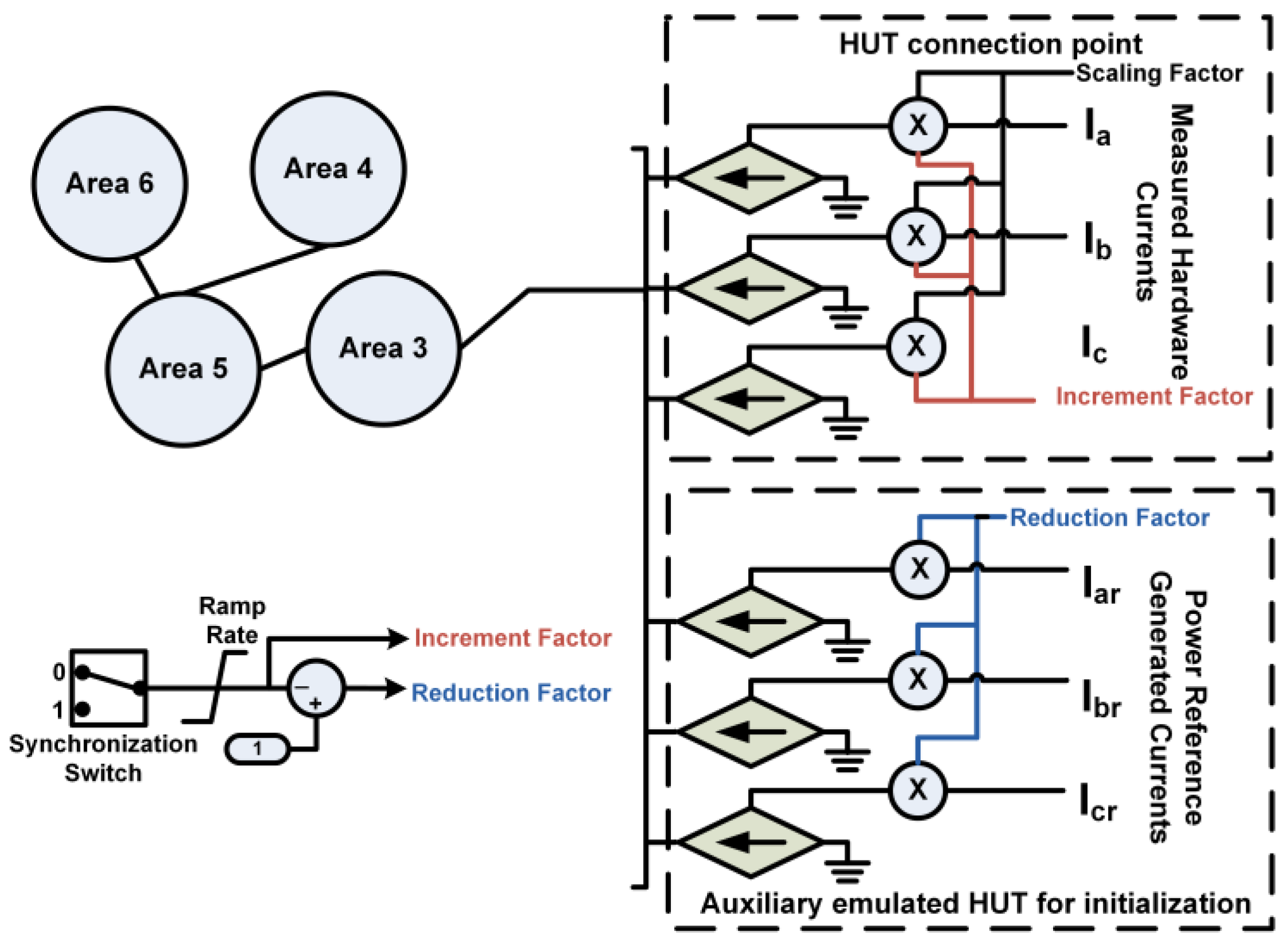
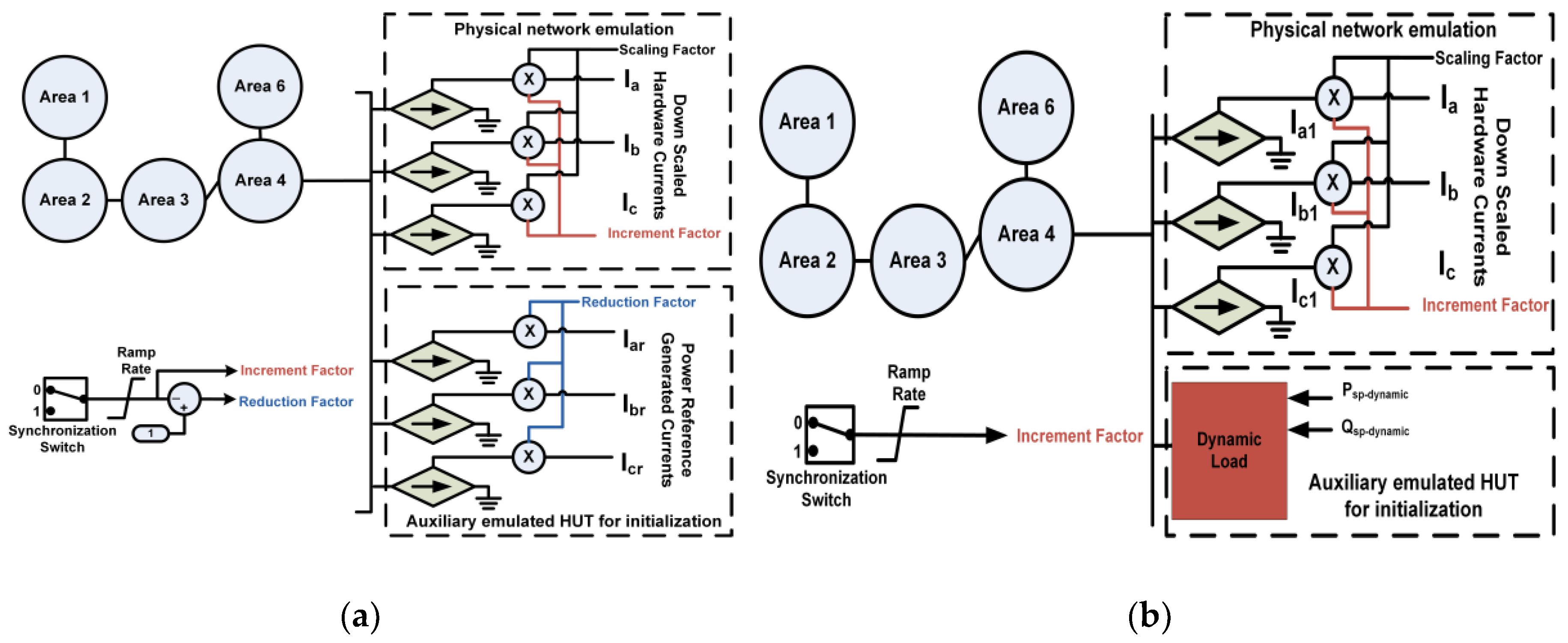
  • AC Controlled Current Source: if a controlled current source is utilized, the synchronization can be achieved with a proposed simple logic as presented in Figure 2. The synchronization process is begun by means of a synchronization switch that inversely ramps up and down both controlled current sources. The ramp rate can be chosen such that it doesn’t create any oscillations or transients on the system, once the currents from the auxiliary emulated HUT are reduced to zero and the currents from the HUT are fully connected to the simulation, the system is synchronized.
From the above discussion, it can be deduced that for the purpose of initialization and synchronization of PHIL setups, where the HUT represents a significant part of the test network, the most convenient option available is to utilize a controlled current source. It performs ideally under all scenarios, with accurate performance and a reliable, straightforward implementation. Furthermore, it is a generic approach that can be utilized when the HUT emulates net generation or load.
A proposed process for performing the initialization and synchronization is shown in Figure 3 with a flowchart. This process assumes that the PHIL simulation is stable for the interface algorithm chosen. This should be ensured before the PHIL simulation initialization and synchronization procedure is begun.

3. Experimental Setup for PHIL

In this section, the different components of the PHIL setup used for the validation of the proposed initialization and synchronization process are described. First the real-time simulation model of the Great Britain (GB) reference power system developed within RSCAD (a power system simulation software from RTDS Technologies, Winnipeg, MB, Canada) is described, the characteristics of the power interface used for the interconnection of the simulated system with the hardware is presented, the HUT utilized is detailed and finally the existing time delay within the setup is considered for the synchronization.

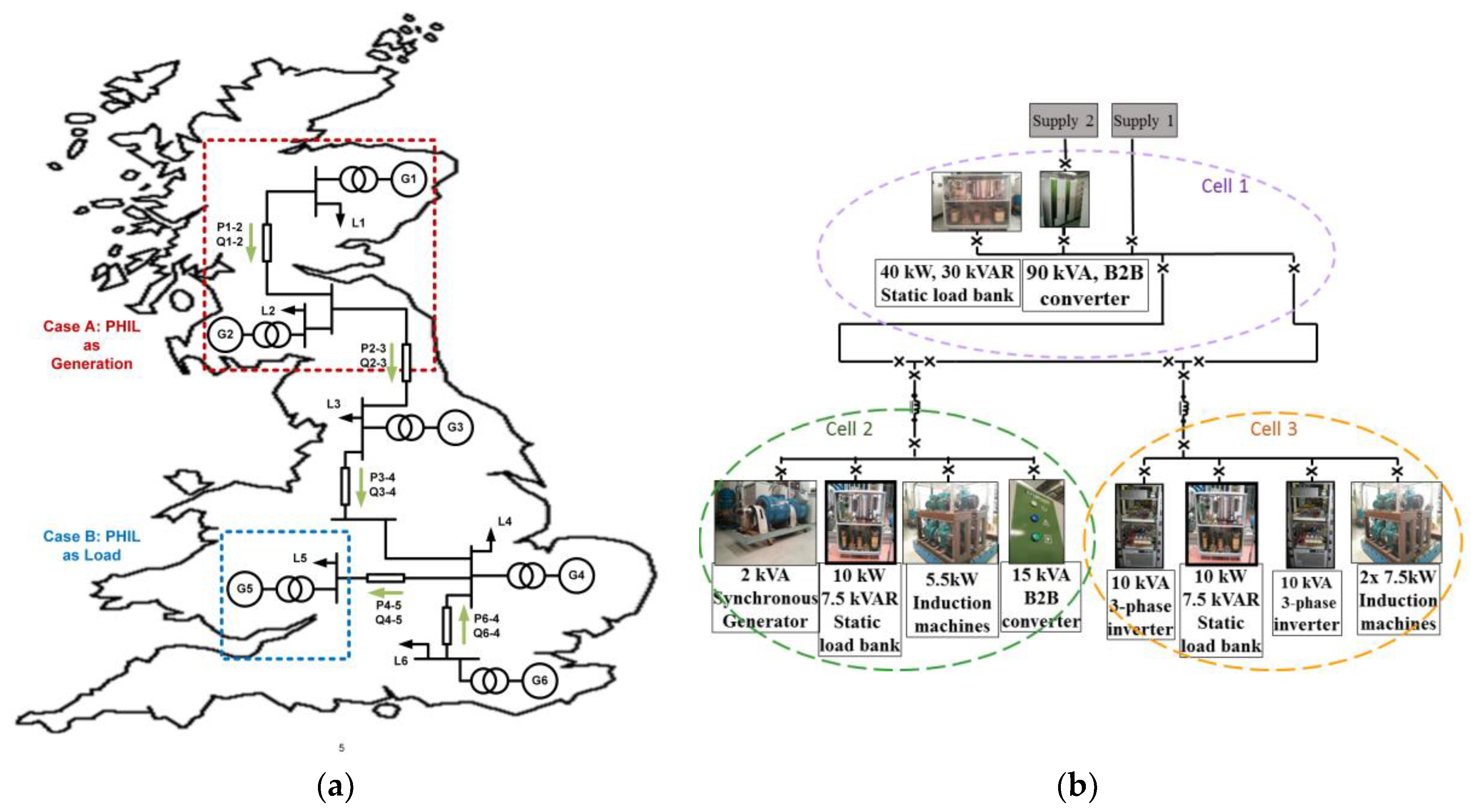
3.1. GB Power System

A reduced six-bus dynamic model of the GB power system has been chosen as the simulated network for this PHIL setup. A single line diagram of the GB power system is shown in Figure 4a. The choice of a six-area model is based on the GB National Electricity Transmission System (NETS) boundary map presented in the Electricity Ten Year Statement (ETYS) of National Grid, Transmission System Operator (TSO) of GB, where the GB transmission network is grouped into six regions [19]. These regions have been developed around major generation sources, power flow corridors and load centres [19]. The model is based on real power flow data of the six regions. Each area is built as the combination of a lumped generator and load. The area wise generation, area wise active and reactive power load, and inter-area power flows have been presented in Table 1 and Table 2. The model has been developed in RSCAD and simulated in real-time using a Real Time Digital Simulator from RTDS Technologies.

3.2. Power Interface

The power interface is composed of a 90 kVA back-to-back converter unit with a switching frequency of 8 kHz responsible for amplifying the signal received from the DRTS. Different interface algorithms have been described in the literature [11,17,20,21]. For the purpose of this paper, the voltage ideal transformer method (ITM) has been selected due to its straightforward implementation and good stability performance. Accordingly, the power interface amplifies and reproduces the voltages received from the simulation and therefore is controlled as a voltage source. At the same time, in the configuration used for this experiment, the power interface is also responsible for measuring the response of the HUT and sending it back to the DRTS for closing the loop with the simulation. Having analog-to-digital and digital-to-analog conversions at both ends, analog interface signals are exchanged between the power interface and the DRTS.

3.3. HUT

The Dynamic Power Systems Laboratory (DPSL) will be utilized as the HUT within this paper for the example case study. DPSL comprises a reconfigurable 125 kVA, 400 V three-phase AC power network with multiple controllable supplies and loads with flexible control systems and interfaces. The one-line diagram of DPSL is presented in Figure 4b. The laboratory network is designed such that it can be split into three separate power islands (represented as cells in Figure 4b) under independent control, or as a centralized interconnected system.
For the example case study, only cell 2 and 3 of Figure 4b will form the HUT, while the 90 kVA unit from cell 1 will represent the power interface. Since the laboratory equipment is relatively small compared to the required power transfers at the PCC, the response of the HUT (the measured currents at the hardware PCC) will be scaled up proportionally to match the test scenario.
The scaling of the response does not impact the simulation results; however, the scaling of the response does make the system more sensitive to oscillations. Small oscillations within the HUT can result in large power oscillations within the simulated system. This can lead the system to instability or cause the implemented controllers to malfunction. This further demonstrates the need for appropriate measures to be undertaken for initialization and synchronization of large synchronous power systems that become sensitive to oscillations under scaled PHIL setups.

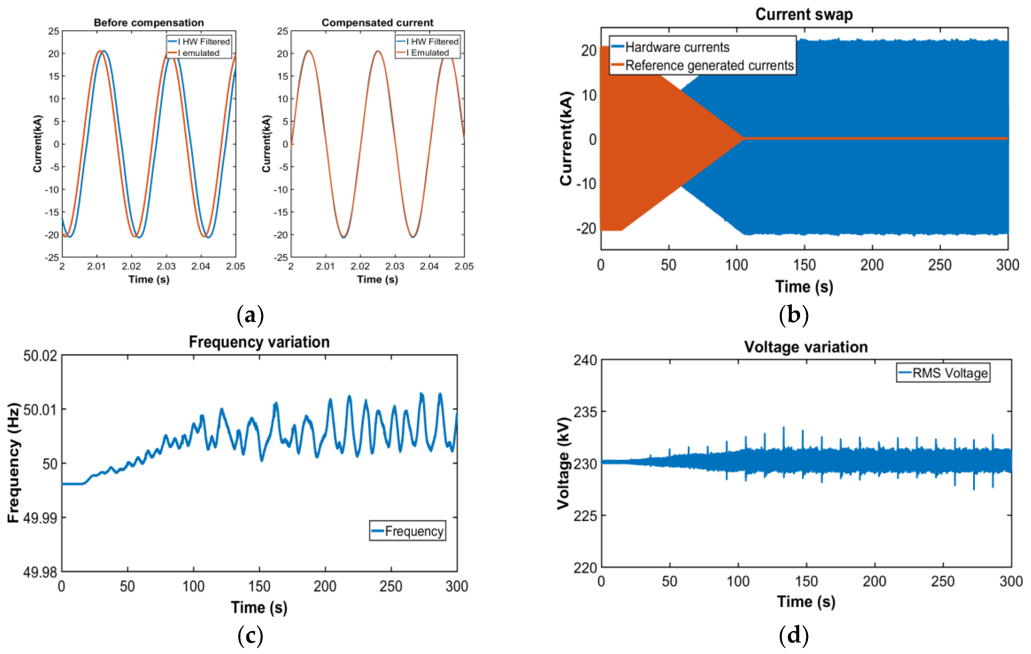
3.4. Time Delay Compensation

The synchronization process is completed when the measured response of the HUT is injected into the simulation. However, typically the hardware response (measured currents at the PCC) is delayed compared to the reference currents generated during initialization. The entire PHIL process: the processing time of the DRTS, the communication between DRTS and power interface, the power interface processing time for amplifying the signal and the feedback loop measurement and communication, contributes to this delay. For this work, a phase compensation method, as reported in [22], is utilized for compensating the time delay. If the delay is not compensated, it is not possible to ensure the equality of the reference power and the injected power and therefore the fidelity of the simulation. Once the delay has been accounted for, the hardware and simulation can be accurately synchronized.

4. Experimental Assessment and Validation

In this section, an assessment of the proposed initialization and synchronization procedures for PHIL simulations is performed. Two case studies have been developed for this purpose, first a case with a significant HUT that affects the PHIL initialization and synchronization if no measure is in place, and afterwards a case in which the simulation could be initialized without HUT, although with erroneous voltage and frequency parameters.
Case Study A: HUT critical for the stability of the real-time simulation.
For the first case study, the HUT is to represent Area 1 and 2 of the GB power system (as shown in Figure 4a) while the remaining areas will be part of the simulated network on the DRTS. As can be observed from Table 2, there is an active and reactive power flow from Area 2 to Area 3. This power flow needs to be matched by the HUT, effectively emulating generation of active and reactive power. Cell 2 and Cell 3 of the DPSL represent Area 2 and Area 1 respectively, while the 90kVA back-to-back converter is used as the power interface.
Initialization
The active and reactive power flow from Area 2 to Area 3 is 8900 MW and 4257 MVAR. Without the HUT representing Area 1 and 2, the remainder of the simulated GB power system (Area 3–6) within RSCAD, fails to initialize due to a lack of generation supposed to be produced by Area 1 and 2. The HUT emulates a large generation portion and the DRTS simulation model is unstable without the HUT. Hence, the process shown in Figure 3 is followed, were initialization of the RT system with an initialization technique is required. The AC current source mode for initialization is implemented due to its simplicity and its suitability to perform the synchronization process.
The schematic of the used methodology for initialization and synchronization of this PHIL implementation is shown in Figure 2. As can be observed from the figure, the auxiliary emulated HUT (the controlled current source in this case) is utilized to reproduce currents generated from the power reference i.e., 8900 MW and 4257 MVAR. Once the RT simulation is initialized and attained steady state, the PCC voltages (scaled down to 400 V) are reproduced in the laboratory using the power interface. Trying to reproduce the simulation voltages when the simulation is not yet stabilized or initialized properly, can damage the hardware components as large transients or/and oscillations can be present. With stable voltage being reproduced at the laboratory, the HUT components are then connected and initialized.
Synchronization
The main objective of the synchronization is to replace the auxiliary currents generated by the controlled current sources with the measured HUT currents. This is intended to be performed so that there is least change in frequency and voltage during the process of synchronization and least impact on the stability of the simulated network. After the DRTS is successfully initialized, the voltage from the simulation is reproduced by the power interface, allowing for the set reference power to be injected into the PCC. In this case, the net generation is produced by the 15 kVA back-to-back converter, the synchronous generator in cell 1 and the 10 kVA inverter in cell 2. A load bank has been added in each of the cells to represent the local loads within the two areas. By using these three power sources, the maximum power injection is limited to 27 kVA. The parameters used for the different hardware components are listed in Table 3. In order to represent the 8900 MW and 4257 MVAR from Area 2, the hardware currents are scaled by means of a scaling factor. For this work the scaling factor is chosen as k = 9 × 10⁵.
Consequently, the measured HUT currents, when injected into the simulation, should be equal to the auxiliary emulated HUT currents. In this case, the currents are being generated by small scale power converters which produce a considerable number of harmonics. The amplitude of the harmonic components when scaled up is not typical of transmission levels. To mitigate this issue, the currents received at the DRTS are filtered by means of a low pass filter. The low pass filter cut off frequency is selected as 200 Hz in order to reduce the impact of the harmonics, thereby alleviating the sensitivity of the simulation to oscillations. However, the low pass filter increases the time delay of the received signal. Therefore, time delay compensation is required not only to compensate for the delay characteristics of PHIL structures, but more importantly in this case, the delay introduced by the filter. This is because the selected cut-off frequency attains a much larger delay than the typical delay of PHIL setups. The results for the compensation of the time delay in this implementation are presented in Figure 5a.
Once the measured hardware currents (after scaling) and the auxiliary signals used for initialization are of the same magnitude and phase, the replacement process is initiated by means of the synchronization switch shown in Figure 2. The currents are then ramped up and down simultaneously over a period of 90 s as shown in Figure 5b. The frequency and voltage at PCC, during the process of synchronization, are presented in Figure 5c,d respectively. As can be observed from the two figures, although the HUT currents have been compensated for the time delay and filter delay and are approximately similar to the emulated currents (as shown in Figure 5a), there is an obvious change in both voltage and frequency during the process of synchronization. The change in frequency is less than 0.02% and the change in voltage is less than 0.05%. This is mainly due to small inaccuracies such as losses in small impedances, measurements inaccuracies and control inaccuracies of the hardware assets, although in this case the difference is not affecting to the test implementation.
The ramp rate utilized plays an important practical role in minimizing such impacts during the process of synchronization. Synchronizing without a ramp rate, risks transients being introduced. The ramp rate is dependent upon the acceptable variation on voltage and frequency during the process of synchronization. With the PHIL simulation fully synchronized and the power transfers set as required by the scenario, the testing of, for example, new control algorithms in a more realistic environment is made possible.
Case Study B: HUT Affecting Voltage and Frequency During Initialization.
For the second case study, the HUT represents Area 5 of the GB power system (as shown in Figure 4a). As can be observed from Table 2, there is an active and reactive power flow into Area 5. Therefore, in this case, the HUT effectively emulates a consumer area at the PCC. Cell 2, Cell 3, and the 40 kVA load bank of Cell 1 combined represent Area 4, while the 90 kVA power converter from Cell 1 is used as the power interface. The specific setpoints used for each of the components in each cell are presented in Table 4.
Initialization
The schematic of the PHIL interconnection within RSCAD is presented in Figure 6a. The HUT emulates net consumption, and so the measured current will have opposite direction to case A and will be drawing power from the simulated power system (through the power interface). In order to represent the 13,080 MW and 7088 MVAR absorbed by Area 5, the hardware currents are scaled by means of a scaling factor. The scaling factor in this case is set to k = 5 × 10⁵.
In this case, the remainder of the GB power system (Areas 1–3, 4 and 6) simulated within RSCAD would initialize without Area 5, as there is enough generation to support the network, unlike case A, but the frequency of the network would be above nominal (as no dispatching algorithm is implemented). The value of the frequency deviation would depend upon the droop settings. This is again undesirable as this would activate any frequency control algorithms implemented within the network. There is, of course, an option to de-activate the control during the process of synchronization. However, there might be hardware limitations on the value of frequency that can be sustained/emulated within the laboratory. To avoid such risks, an auxiliary component should be utilized to initialize the test network for PHIL simulations. A dynamic load or a controlled current source can be used for this purpose.
The schematic for initialization and synchronization of PHIL at the RTDS with the current source as the initialization and synchronization component is shown in Figure 6a. The reference currents for the auxiliary current source can be generated as presented in Case A Initialization. A dynamic load could be also used for the initialization, however depending on the simulation software used this can have different forms. For example, within Simulink simulation software the dynamic load is equivalent to a current source, hence the method would be equivalent to the current source method presented before (and therefore can be utilized for case A and B), while within RSCAD (RTDS simulation software tool) the dynamic load model does not allow for negative power set points (rendering it unusable for case A).
Synchronization
If the current sources are used for the initialization, the same process of synchronization as presented in Case A Synchronization is used. In this case, the dynamic load model could also be utilized indistinctly. However, if a dynamic load is being utilized, instead of using current set points, active and reactive power set points are required (as presented in Figure 5b), and these can be calculated as:
P S P _ d y n a m i c = P r e f P H W
Q S P _ d y n a m i c = Q r e f Q H W
where PHW and QHW are the active and reactive power drawn by the hardware respectively, and can be calculated as:
P H W = V a I a 1 + V b I b 1 + V c I c 1
Q H W = 1 3 ( V a ( I b 1 I c 1 ) + V b ( I c 1 I a 1 ) + V c ( I a 1 I b 1 ) )
where Vabc are the three phase voltages at PCC and Iabc1 are the currents measured at the PCC after the increment factor.
For this scenario, the current source model has been implemented. It can be observed from Figure 7 that by initializing and synchronizing the PHIL implementation with the current sources, the frequency and voltage at the PCC remain at the same steady state levels as before the connection with the HUT. Also, due to the nature of the hardware used and the real measurement devices, which can introduce some noise into the signals, the frequency and voltage waveforms show more realistic dynamics in comparison with a pure simulation.

5. Conclusions

PHIL simulations can be complex to initialize and synchronize depending on the HUT and its significance to the dynamic behaviour and stability of the overall study system. This then represents a limiting factor on the range of scenarios for which PHIL can be applied. This paper presents a range of possible methodologies for enabling the initialization and synchronization of such scenarios. The investigation of these alternatives has led to the identification of a recommended approach that uses current sources for initialization and symmetrical ramping rates for synchronization of PHIL simulations. The resulting improved performance and extended range of feasible scenarios that can be studied have been validated by experimentation of two different and realistic scenarios for the GB power system. This will allow for safer and more stable PHIL simulations, and permit validation of a wider range of realistic simulations through PHIL to the betterment of new controllers and power components.

Author Contributions

E.G.-S. and M.H.S. conceived the research idea, performed the experiments and wrote the paper. A.J.R. and G.M.B. oversaw the work and proofread the paper.

Acknowledgments

This work was partly supported by the European Community’s Horizon 2020 Program (H2020/2014–2020) under the project “ERIGrid: European Research Infrastructure supporting Smart Grid Systems Technology Development, Validation, and Roll Out” (Grant No. 654113) and from the European Union Seventh Framework Programme (FP7) under the project ELECTRA IRP (Grant No. 609687).

Conflicts of Interest

The authors declare no conflict of interest.

References

  1. Strasser, T.; Andrén, F.P.; Lauss, G.; Bründlinger, R.; Brunner, H.; Moyo, C.; Seitl, C.; Rohjans, S.; Lehnhoff, S.; Palensky, P.; et al. e & i Elektrotechnik und Informationstechnik; Springer: Vienna, Austria, 2017; Volume 134, pp. 71–77. [Google Scholar]
  2. Kotsampopoulos, P.C.; Lehfuss, F.; Lauss, G.F.; Bletterie, B.; Hatziargyriou, N.D. The Limitations of Digital Simulation and the Advantages of PHIL Testing in Studying Distributed Generation Provision of Ancillary Services. IEEE Trans. Ind. Electron. 2015, 62, 5502–5515. [Google Scholar] [CrossRef]
  3. Edrington, C.S.; Steurer, M.; Langston, J.; El-Mezyani, T.; Schoder, K. Role of Power Hardware in the Loop in Modeling and Simulation for Experimentation in Power and Energy Systems. Proc. IEEE 2015, 103, 2401–2409. [Google Scholar] [CrossRef]
  4. Kotsampopoulos, P.; Kleftakis, V.; Messinis, G.; Hatziargyriou, N. Design, development and operation of a PHIL environment for Distributed Energy Resources. In Proceedings of the IECON 2012—38th Annual Conference on IEEE Industrial Electronics Society, Montreal, QC, Canada, 25–28 October 2012; pp. 4765–4770. [Google Scholar]
  5. Ren, W.; Steurer, M.; Woodruff, S. Applying Controller and Power Hardware-in-the-Loop Simulation in Designing and Prototyping Apparatuses for Future All Electric Ship. In Proceedings of the 2007 IEEE Electric Ship Technologies Symposium, Arlington, VA, USA, 21–23 May 2007; pp. 443–448. [Google Scholar]
  6. Langston, J.; Schoder, K.; Steurer, M.; Faruque, O.; Hauer, J.; Bogdan, F.; Bravo, R.; Mather, B.; Katiraei, F. Power hardware-in-the-loop testing of a 500 kW photovoltaic array inverter. In Proceedings of the IECON 2012—38th Annual Conference on IEEE Industrial Electronics Society, Montreal, QC, Canada, 25–28 October 2012; pp. 4797–4802. [Google Scholar]
  7. Naeckel, O.; Langston, J.; Steurer, M.; Fleming, F.; Paran, S.; Edrington, C.; Noe, M. Power Hardware-in-the-Loop Testing of an Air Coil Superconducting Fault Current Limiter Demonstrator. IEEE Trans. Appl. Superconduct. 2015, 25, 1–7. [Google Scholar] [CrossRef]
  8. Kotsampopoulos, P.; Hatziargyriou, N.; Bletterie, B.; Lauss, G.; Strasser, T. Introduction of advanced testing procedures including PHIL for DG providing ancillary services. In Proceedings of the IECON 2013—39th Annual Conference of the IEEE Industrial Electronics Society, Vienna, Austria, 10–13 November 2013; pp. 5398–5404. [Google Scholar]
  9. Zhu, K.; Chenine, M.; Nordstrom, L. ICT Architecture Impact on Wide Area Monitoring and Control Systems’ Reliability. IEEE Trans. Power Deliv. 2011, 26, 2801–2808. [Google Scholar] [CrossRef]
  10. Lauss, G.F.; Faruque, M.O.; Schoder, K.; Dufour, C.; Viehweider, A.; Langston, J. Characteristics and Design of Power Hardware-in-the-Loop Simulations for Electrical Power Systems. IEEE Trans. Ind. Electron. 2016, 63, 406–417. [Google Scholar] [CrossRef]
  11. Ren, W.; Steurer, M.; Baldwin, T.L. Improve the Stability and the Accuracy of Power Hardware-in-the-Loop Simulation by Selecting Appropriate Interface Algorithms. IEEE Trans. Ind. Appl. 2008, 44, 1286–1294. [Google Scholar] [CrossRef]
  12. Viehweider, A.; Lauss, G.; Felix, L. Stabilization of Power Hardware-in-the-Loop Simulations of Electric Energy Systems. Simul. Model. Pract. Theory 2011, 19, 1699–1708. [Google Scholar] [CrossRef]
  13. Hatakeyama, T.; Riccobono, A.; Monti, A. Stability and accuracy analysis of power hardware in the loop system with different interface algorithms. In Proceedings of the 2016 IEEE 17th Workshop on Control and Modeling for Power Electronics (COMPEL), Trondheim, Norway, 27–30 June 2016; pp. 1–8. [Google Scholar]
  14. Dargahi, M.; Ghosh, A.; Ledwich, G. Stability synthesis of power hardware-in-the-loop (PHIL) simulation. In Proceedings of the 2014 IEEE PES General Meeting | Conference & Exposition, National Harbor, MD, USA, 27–31 July 2014; pp. 1–5. [Google Scholar]
  15. Brandl, R. Operational Range of Several Interface Algorithms for Different Power Hardware-In-The-Loop Setups. Energies 2017, 10, 1946. [Google Scholar] [CrossRef]
  16. Liegmann, E.; Riccobono, A.; Monti, A. Wideband identification of impedance to improve accuracy and stability of power-hardware-in-the-loop simulations. In Proceedings of the 2016 IEEE International Workshop on Applied Measurements for Power Systems (AMPS), Aachen, Germany, 28–30 September 2016; pp. 1–6. [Google Scholar]
  17. Lehfuss, F.; Lauss, G.; Strasser, T. Implementation of a multi-rating interface for Power-Hardware-in-the-Loop simulations. In Proceedings of the IECON 2012—38th Annual Conference on IEEE Industrial Electronics Society, Montreal, QC, Canada, 25–28 October 2012; pp. 4777–4782. [Google Scholar]
  18. Yu, M.; Roscoe, A.J.; Dyśko, A.; Booth, C.D.; Ierna, R.; Zhu, J.; Urdal, H. Instantaneous Penetration Level Limits of Non-Synchronous Devices in the British Power System. IET Renew. Power Gener. 2016, 11, 1211–1217. [Google Scholar] [CrossRef]
  19. National Grid. Electricity‎ Ten‎ Year‎ Statement 2016; ‎National Grid: Warwick, UK, 2016. [Google Scholar]
  20. Lentijo, S.; D’Arco, S.; Monti, A. Comparing the Dynamic Performances of Power Hardware-in-the-Loop Interfaces. IEEE Trans. Ind. Electron. 2010, 57, 1195–1207. [Google Scholar] [CrossRef]
  21. De Jong, E.; de Graff, R.; Vassen, P.; Crolla, P.; Roscoe, A.; Lefuss, F.; Lauss, G.; Kotsampopoulos, P.; Gafaro, F. European White Book on Real-Time Power Hardware in the Loop Testing; DERlab: Kassel, Germany, 2012. [Google Scholar]
  22. Guillo-Sansano, E.; Roscoe, A.J.; Burt, G.M. Harmonic-by-harmonic time delay compensation method for PHIL simulation of low impedance power systems. In Proceedings of the 2015 International Symposium on Smart Electric Distribution Systems and Technologies (EDST), Vienna, Austria, 8–11 September 2015; pp. 560–565. [Google Scholar]
Figure 1. PHIL implementation.
Energies 11 01087 g001
Figure 2. PHIL initialization and synchronization structure at DRTS side.
Energies 11 01087 g002
Figure 3. Initialization and synchronization flowchart.
Energies 11 01087 g003
Figure 4. (a) Reduced six-bus dynamic model of the GB power system, (b) Dynamic power system laboratory (HUT).
Energies 11 01087 g004
Figure 5. Results for study case A: HUT critical for stability of RT simulation, (a) time delay compensation, (b) currents swapping during synchronization, (c) frequency at PCC during synchronization and (d) voltage at PCC during synchronization.
Energies 11 01087 g005
Figure 6. PHIL configuration for case study B: affecting voltage and frequency during initialization. (a) with current source, (b) with dynamic load.
Energies 11 01087 g006
Figure 7. Results for case B: affecting voltage and frequency during initialization (a) Frequency variation, (b) voltage variation.
Energies 11 01087 g007
Table 1. Area wise capacity and initial load condition.
Capacity and Loading ConditionsArea 1Area 2Area 3Area 4Area 5Area 6
Area wise generation capacity (MVA)11,00020,0009160550015,5002000
Area wise active power load (MW)846812,5488398215026,852100
Area wise reactive power load (MVAr)410960774067104113,005500
Table 2. Inter-area power flows.
Inter-area active power flow (MW)P1-2P2-3P3-4P4-5P6-4
20978900910513,080970
Inter-area reactive power flow (MVAr)Q1-2Q2-3Q3-4Q4-5Q6-4
1328425750257088155
Table 3. Power setpoints for hardware components for case study A.
AreaComponentP (W)Q (Var)
Cell 215 kVA B2B Inverter70003600
2 kVA Synchronous Generator15000
Load Bank 2−15000
Cell 310 kVA Inverter66001100
Load Bank 3−33000
Table 4. Power setpoints for hardware components for case study B.
AreaComponentP (W)Q (Var)
Cell 1Load Bank 1−14,000−7900
Cell 215 kVA B2B Inverter4500−3000
2 kVA Synchronous Generator10000
Load Bank 2−9000−3500
Cell 310 kVA Inverter52000
Load Bank 3−9000−3500
Induction motor−4700−3000

