Article

Analysis of Capacitance to Ground Formulas for Different High-Voltage Electrodes

by
Jordi-Roger Riba
1,* and
Francesca Capelli
2
1
Electrical Engineering Department, Universitat Politècnica de Catalunya, 08034 Barcelona, Spain
2
Department of Research & Development, SBI Connectors España, 08635 Barcelona, Spain
*
Author to whom correspondence should be addressed.
Energies 2018, 11(5), 1090; https://doi.org/10.3390/en11051090
Submission received: 27 March 2018 / Revised: 20 April 2018 / Accepted: 24 April 2018 / Published: 28 April 2018
(This article belongs to the Section F: Electrical Engineering)

Abstract

:
Stray capacitance can seriously affect the behavior of high-voltage devices, including voltage dividers, insulator strings, modular power supplies, or measuring instruments, among others. Therefore its effects must be considered when designing high-voltage projects and tests. Due to the difficulty in measuring the effects of stray capacitance, there is a lack of available experimental data. Therefore, for engineers and researchers there is a need to revise and update the available information, as well as to have useful and reliable data to estimate the stray capacitance in the initial designs. Although there are some analytical formulas to calculate the capacitance of some simple geometries, they have a limited scope. However, since such formulas can deal with different geometries and operating conditions, it is necessary to assess their consistency and applicability. This work calculates the stray capacitance to ground for geometries commonly found in high-voltage laboratories and facilities, including wires or rods of different lengths, spheres and circular rings, the latter ones being commonly applied as corona protections. This is carried out by comparing the results provided by the available analytical formulas with those obtained from finite element method (FEM) simulation, since field simulation methods allow solving such problem. The results of this work prove the suitability and flexibility of the FEM approach, because FEM models can deal with wider range of electrodes, configurations and operating conditions.

1. Introduction

The calculation of capacitance formulas has received little attention compared to the analysis of inductance calculation formulas [1,2]. Nearby surfaces separated by an insulating medium such as air, subjected to different electric potentials, induce a stray or parasitic capacitance, and therefore this configuration acts as a capacitor. High voltages and high frequencies tend to amplify the effects of the unwanted stray capacitance. The analysis of stray capacitance effects is of interest in different disciplines, including electrical engineering, high-voltage applications, radio engineering or physical sciences, among others [3].
Different studies prove that the stray capacitance produces an uneven voltage distribution across each insulator unit in a high-voltage insulator string [4,5]. The effect of the stray capacitance is to reduce the efficacy of each additional insulator unit due to the non-linear voltage distribution [6]. This is because the capacitive current and the corresponding voltage drop across each insulator unit are greater in the insulator units closer to the conductors, due to the effect of the distributed stray capacitances to ground [7]. The string elements closer to the line are subjected to a higher electrical stress than those closer to the tower. Grading rings can be used at both ends of the string to homogenize the voltage drop across each insulator unit [8]. A similar effect occurs in high-voltage switching mode power supplies composed of several modules in series, since in [9] it is proved that the stray capacitance to ground has a significant impact on the individual voltage of each module. In other high-voltage applications, including high-voltage transformers [10] or high-voltage motors, parasitic capacitances have a key role to predict the frequency behavior of such machines.
Accurate methods to calculate the capacitance are based on the calculation of the electrostatic field generated by the system of charged objects under consideration [3]. The capacitance of basic isolated geometries, such as very long horizontal cylindrical conductors, coaxial cylindrical conductors, concentric spheres, or spheres well above ground, can be easily deduced theoretically. However, such formulas have very restricted practical use. The calculation of the capacitance of conductive objects which are close to ground leads to challenging mathematical problems, even for simple geometries. Therefore, analytical solutions for capacitance only exist for a limited number of electrode geometries and configurations, which have almost no practical applications [11], and often only contemplate the stray capacitance to ground, thus disregarding the effects of nearby grounded electrodes, structures or walls [3].
As a consequence, computational methods are increasingly being applied to solve such problem, although most of the published works deal with very particular problems, such as insulator strings [4,5,7], transformer windings [10] or voltage dividers [12], among others. FEM is perhaps the most applied computational technique to calculate the effects of capacitance, since it allows dealing with complex three-dimensional geometries, as reflected in several works [13,14,15,16,17,18,19].
Since stray capacitances are not easily measurable, because of the low immunity to noise of the small signal to be acquired [20], results provided by numerical methods are a good alternative during the design stage of high-voltage devices and instruments. Therefore, the capacitance between energized electrodes or between electrodes and ground is a factor to be considered when designing and planning high-voltage projects and tests [11].
Most works analyze specific problems related to the unwanted effects of stray capacitance, such as in transformer windings [10], motor windings [21] or insulator strings [
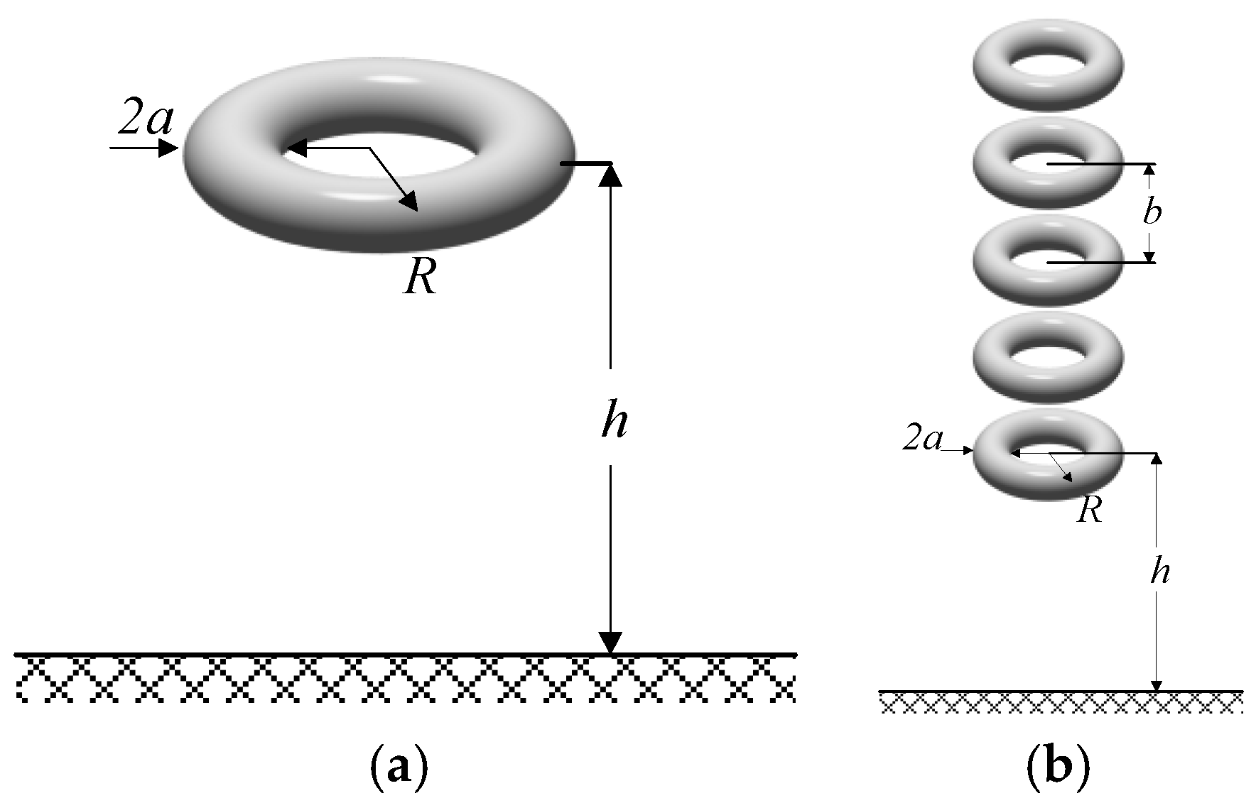
7], among others. However, there are no recent works providing a systematic account of the problems to calculate the stray capacitance to ground for geometries found in high-voltage laboratories and high-voltage installations such as substations. These geometries include wires, rods, spheres, and circular rings, the latter ones being commonly applied as corona protections. The stray capacitances due to these high-voltage electrodes can have a non-negligible impact on the measurement results and behavior of the devices involved.
This paper is focused to review and analyze the accuracy of different formulas found in the technical literature to calculate the stray capacitance to ground of various high-voltage electrodes. To this end, due to the lack of available experimental data because of experimental difficulties related to the small signal to be acquired and noise immunity, the results provided by the formulas are compared with the results provided by FEM simulations. It is noted that regardless the impact of the stray capacitance in high-voltage applications, at our knowledge, there are no published technical works assessing the accuracy of such formulas; thus this work contributes in this area. Results presented prove that FEM models offer flexibility, simplicity and accuracy to analyze the effects of stray capacitance in high-voltage systems with different geometries.

2. The FEM Approach to Analyze the Stray Capacitance

The stray capacitance to ground is directly related to the distribution of the electric field around high-voltage electrodes [22]. It is a recognized fact that the effects of stray capacitance can be determined by means of FEM-based approaches [12,23].
The capacitance can be calculated from the ratio C = Q/U, defined by the charge Q stored in the system and the electric potential U, supposing that the system under analysis is far from other charged bodies [3]. Therefore, the stray capacitance concept arises between any two charged bodies subjected to different electric potentials, and can be important in high-frequency and high-voltage applications.
For low-frequency applications, the capacitance can be calculated by analyzing the energy related to the electrostatic field, thus disregarding the displacement current. To evaluate the capacitance of a given geometry, it is necessary to calculate the electric potential on the surface of the analyzed conductor. Next, the outer electric potential and the electric field are calculated within all points surrounding the conducting electrodes, by applying the potential as boundary condition [14,24]. Finally, the capacitance of the analyzed system is calculated by applying:
C = 2 · W E / U 2
WE being the stored electrostatic energy.
The next paragraphs detail the process to follow for determining the stored electrostatic energy.
From the Gauss law that relates the distribution of the electric charge density (C/m3) to the electric field E (V/m),
( ε · E ) = ρ
and the relationship between the electric field and the electric potential U, E = U , the Poisson’s equation for electrostatics arises [25],
2 U = ρ / ε
Equation (3) allows solving for the electric potential and field in all points of the domain [26]. Next, the energy density in any point of the air domain is calculated as:
u E ( x , y , z ) = 1 2 ε o E ( x , y , z ) 2 ( J / m 3 )
The electrostatic energy stored in the domain can be calculated by integrating the energy density over the volume of the domain outside the conductive high-voltage electrode [14,27]:
W E = 1 2 v ε o · E ( x , y , z ) 2 d x d y d z ( J )
Finally, the capacitance is calculated by applying Equation (1) [24]. Therefore, the capacitance is calculated from the electrostatic energy stored in the air because of the incitation of U.
Figure 1 shows the surface meshes applied to some of the geometries analyzed in this paper, including cylindrical conductors, circular rings and spheres.
Figure 2 shows the blocks and meshes types applied in the simulations. Whereas a sufficiently large outer block was used to set the boundary conditions, a much smaller inner block was used in order to apply a much finer tetrahedral mesh to ensure improved accuracy.
Both three-dimensional (3D) and two-dimensional (2D) FEM simulations were carried out to simulate all geometries analyzed in this work. Whereas 3D-FEM simulations were applied to wires of finite length, circular rings and spheres, 2D-FEM simulations were applied to analyze wires of infinite length. Parametric simulations were carried out to automatically change the value of different parameters, such as the height about ground level or the curvature radius of the different analyzed geometries.
Simulations conducted in this work were performed by means of the Comsol Multiphysics package using the electrostatics module. They consist of approximately 0.5–9.5 million tetrahedral elements, 66–590 thousand triangular elements, 0.5–73 thousand edge elements, and 22–96 vertex elements, depending on the specific geometry analyzed.

3. The Analyzed Geometries

This section analyzes the accuracy of formulas to calculate the capacitance between different electrode geometries and an infinite ground plane, some of them being based on the method of images.

3.1. Finite-Length Straight Round Wire Which Is Parallel to the Ground Plane

Figure 3 shows the layout of a straight conductor of round section which is parallel to a conducting plane.
According to [3], the capacitance of a straight conductor of round section which is parallel to a conducting plane can be approximated as:
C = 2 π ε l ln ( 2 h / a ) 2.303 D 1 ( 0.5 l / h )   ( F )
being the permittivity of air, 8.85 × 10⁻¹² F/m, l the length of the conductor, h the height above ground and D1 a coefficient depending on l/(2h), which is obtained by interpolating the values given in Table 1.
Table 2 compares the capacitance of a finite-length straight round wire, which is parallel to the ground plane, provided by Equation (6) with those obtained by means of FEM simulations.
Data presented in Table 2 show a good agreement between the results provided by Equation (6) and those from FEM simulations.

3.2. Finite-Length Straight Wire of Round Section Which Is Perpendicular to the Ground Plane

According to [3], the capacitance of a straight conductor of round section which is perpendicular to a conducting plane, (see Figure 4) can be approximated as:
C = 2 π ε l ln ( l / a ) 2.303 D 2
D2 being a coefficient, which is calculated by interpolation of the values given in Table 3, as a function of h/l.
Table 4 compares the capacitance of a finite-length straight round wire, which is perpendicular to the ground plane, provided by Equation (7) with those obtained by means of FEM simulations.
Results presented in Table 4 show a good match between the data provided by Equation (7), with the data obtained from FEM simulations, especially when the height h of the conductor above the ground plane increases.

3.3. Infinite-Length Straight Circular Wire Which Is Parallel to a Conducting Plane

By applying the images method, the capacitance per unit length of a round straight conductor of infinite-length, which is parallel to a conducting plane, as shown in Figure 5, can be calculated as [3]:
C / l = 2 π ε acosh ( h / a )   ( F / m )
where a is the radius of the conductor, and h is the distance between its center and the ground plane.
In [28], an equivalent formula is proposed:
C / l = 2 π ε ln ( h + h 2 a 2 a )   ( F / m )
Figure 5 shows an infinite straight conductor of radius a, which is parallel to the ground plane:
Table 5 summarizes the results attained by means of Equations (8), (9) and FEM simulations for different values of the radius a, and the height h. It shows an excellent agreement between the results provided by Equations (8), (9) and FEM simulations.

3.4. Infinite-Length Straight Wire of Square Section Which Is Parallel to a Conducting Plane

By applying the method of the mirror images, the capacitance per unit length of an infinite-length straight conductor of square section, which is parallel to a conducting plane, can be calculated as [3]:
C / l = 4 π ε ln ( x 2 2 x x 1 )   ( F / m )
where x = 3.39 h/a, a being the side length of the square, and h the distance between the geometrical center of the wire and the ground plane.
Figure 6 shows the layout of the analyzed conductor.
Table 6 shows the results attained by applying Equation (10) and FEM for different values of the side length a, and the height h.

3.5. Sphere Over a Conducting Plane

Spheres are frequently applied as corona protections in high-voltage applications, although their stray capacitance can affect the behavior of sensitive high-voltage devices.
Figure 7 shows the layout of a sphere, where r is its radius, and h the distance between the lowest point of the sphere and the ground plane.
By applying the method of the images, the capacitance of a conductive sphere of radius r placed at a height h above a ground plane is given by [29]:
C = 4 π ε r i = 0 2 sin h ( η 0 ) e ( 1 + 2 i ) η 0 1
where η 0 = acos   h ( 1 + h / r ) .
A simplified expression for this arrangement is given in [29] as:
C = 4 π ε r [ 1 + 0.5 log ( 1 + r / h ) ]
An equivalent formulation to Equation (11) was proposed by Snow [28]:
C = 8 π ε r h 2 r 2 n = 0 e ( n + 0.5 ) γ 1 e ( n + 0.5 ) γ
being defined as:
γ = 2 ln ( h + h 2 r 2 r )
and h* = h + r.
Table 7 shows the results obtained by applying Equations (11)–(13) and FEM, for different values of the radius r and the height h.
Results presented in Table 7 show an excellent match between Equations (11), (13) and FEM results, although a greater difference when applying Equation (13), as expected.

3.6. Circular Ring or Toroid Which Plane Is Parallel to a Conducting Plane

Toroidal rings are commonly used as corona protections in high-voltage applications. However, the rings introduce a non-negligible capacitance in the system, whose impact cannot be neglected depending on the application.
Figure 8 shows a toroid of round section which is parallel to a conducting plane and different toroids lying in parallel planes.
By applying the images method, the capacitance of a circular ring or toroid, which is parallel to a conducting plane, can be calculated as [3]:
C = 4 π 2 ε R ln ( 8 R / a ) K ( k 2 ) k   [ F ]
where a and R are, respectively, the minor and major radiuses, h is the distance between the geometrical center of the toroid and the ground plane, k 2 = R 2 R 2 + h 2 and K is the complete elliptic integral of first kind with modulus k2, which can be computed by means of the ellipke function of MATLAB (2017, The MathWorks Ltd., Natick, MA, USA).
Table 8 summarizes the results obtained by applying Equation (15) and FEM, for different values of the radiuses a, R and the height h. It shows a good agreement between the results of both systems.
FEM allows the simple simulation of several concentric corona rings sharing the same vertical axis as shown in Figure 8b. This configuration common applied in high-voltage generators, voltage dividers, or capacitors, among others. However, there are no analytical formulas to deal with this geometry.
Table 9 presents the results obtained by means of FEM simulations, when dealing with a row of five circular rings which are placed as shown in Figure 8b.

3.7. n Parallel Round Wires of Finite Length Lying in a Plane Parallel to the Ground Plane

According to [3], the capacitance of n parallel round conductors of finite length lying in the same plane, which is parallel to the ground plane, can be calculated as:
C = 2 π ε n l ln ( 2 h / a ) + ( n 1 ) ln ( 2 h / b ) 2.303 n [ D 1 ( 0.5 l / h ) + B n ]
a being the radius of the conductors, l the length of any conductor, h the distance between the center of any conductor and the ground plane, b the distance between the centers of two adjacent conductors, and Bn a coefficient, which is calculated as:
B n = 2 n 2 [ log ( n 1 ) + 2 log ( n 2 ) + 3 log ( n 3 ) + ( n 2 ) log 2 ]
The values of D1 (0.5l/h) are given in Table 1. It is noted that Equation (16) is not a general formula, since it is only valid when bl/(n−1).
When the distance dk (k = 1, 2, …, n−1) between any two wires is inferior than the mean height above the ground plane, that is, dk << h, [3] suggests to apply:
C = 2 π ε n l 2.303 F 1
F1 being calculated as:
F 1 = log ( 2 h / a ) + k = 1 n 1 [ log ( 2 h / d k ) + 0.434 ( d k / l ) ] n D 1
Figure 9 shows the layout of the n parallel round wires of finite length, lying in a plane parallel to the ground plane.
Table 10 summarizes the results obtained by applying Equations (16), (18) and FEM, for different values of the radius a, the length l, and the height h.
According to the results summarized in Table 10, FEM results are more general results. FEM simulations avoid the inherent limitations and applicability of Formulas Equations (16) and (18), since they are not general, and only provide accurate results when fulfilling some constraints.

3.8. n Identical Straight Wires of Finite Length Parallel to the Ground Plane and Arranged on the Surface of a Circular Cylinder

According to [3], the capacitance of n identical straight wires of finite length parallel to the ground plane, and arranged on the surface of a circular cylinder, is given by Equation (18). It is noted that the coefficients D1 (0.5l/h) and dk (distance between the centers of any two wires) included in Equation (19) are obtained from Table 1, and by applying d k = 2 R sin ( k π / n ) with k = 1, 2, 3, …, n−1, respectively. It is known that Equation (18) is not accurate when the distance dk (k = 1, 2, …, n−1) between any two wires is inferior than the height of any conductor above the ground plane, that is, dk << h.
Figure 10 shows n straight round conductors of finite length (radius a, length l) parallel to the ground plane, which are placed on the surface of a circular cylinder of radius R whose center is placed at a height h above the ground plane.
Table 11 summarizes the results obtained by applying Equation (20) and FEM, for different values of the radius a, the length l, and the height h.
Results summarized in Table 11 prove that the accuracy of Equation (18) lowers when reducing the height of the conductors above the ground plane.

4. Discussion

This section summarizes the results attained in this work. As deduced from Section 3, FEM simulations offer more flexibility, generalization capability, and the possibility to deal with more complex geometries than analytical formulas for calculating the stray capacitance of high-voltage electrodes to ground. Although analytical formulas only are available for some simple geometries, they can be effectively applied to determine the straight capacitance to ground of high-voltage electrodes with simple geometries.
Table 12, Table 13 and Table 14 summarize the main results attained in this work.
Results summarized in Table 12 clearly show a very good agreement between the results provided by analytical formulas and FEM simulation for wires of infinite length, whereas in the case of straight wires of finite length, maximum differences around 1–5% are found.
Results presented in Table 13 clearly show that in the case of spheres, analytical and FEM results are almost the same, whereas in the case of circular rings, maximum differences around 5–8% are found.
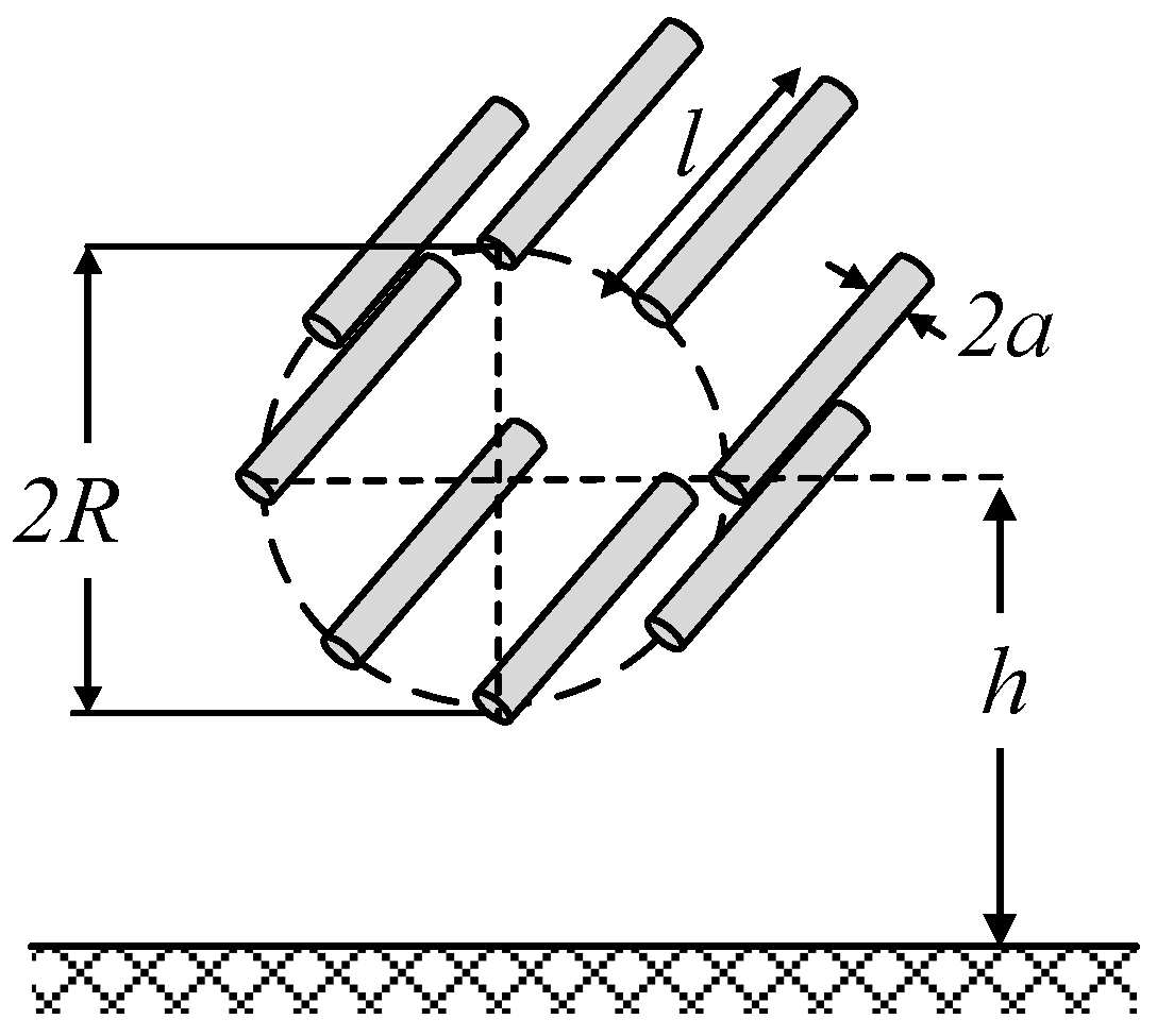
When dealing with multi-wire configurations, the differences are much higher than in the geometries above, since differences around 5–56% can be found. In addition, for some geometries, the analytical formulas available for multi-wire geometries cannot be applied, since some of the input parameters are out of the applicability limits of such formulas.

5. Conclusions

This work has analyzed the behavior of several approximate and exact formulas to calculate the capacitance to ground of high-voltage electrodes with different geometries. Due to experimental difficulties involved, there is a lack of experimental data, so it is necessary to develop numerical methods to infer the value of the capacitance when designing high-voltage tests and projects. The analyzed geometries found in high-voltage applications include different combinations of wires and rods, spheres and circular rings, the latter two being commonly applied as corona protections in high-voltage projects. The results provided by the analyzed formulas have been compared against the results provided by FEM simulations, since FEM simulations are internationally recognized as a valid means of obtaining accurate and reliable data. The analysis performed in this work has proved the inherent limitations of the analyzed formulas. It has been proved that although in some configurations the results are very accurate (single straight wires or single sphere configurations), while in other cases important differences arise, especially when dealing with multi-wire configurations. The stray capacitance of a multi-toroid geometry has been also analyzed, which cannot be calculated by means of analytical formulas. Therefore, this work has proven that analytical formulas can only deal with a narrow number of geometries, and has also proven the enhanced performance and flexibility of FEM simulations, due to their suitability, flexibility, and the wider range of geometries that FEM simulations allow to be evaluated.

Author Contributions

Jordi-Roger Riba conceived and designed the numerical tests, analyzed the data and wrote the paper; Francesca Capelli performed the simulations.

Conflicts of Interest

The authors declare no conflict of interest.

References

  1. Capelli, F.; Riba, J.-R. Analysis of formulas to calculate the AC inductance of different configurations of nonmagnetic circular conductors. Electr. Eng. 2016, 99, 827–837. [Google Scholar] [CrossRef]
  2. Morgan, V.T. The Current Distribution, Resistance and Internal Inductance of Linear Power System Conductors—A Review of Explicit Equations. IEEE Trans. Power Deliv. 2013, 28, 1252–1262. [Google Scholar] [CrossRef]
  3. Iossel, Y.Y.; Kochanov, E.S.; Strunskiy, M.G. The Calculation of Electrical Capacitance; Foreign Technology Div Wright-Patterson Afb Oh: Springfield, VA, USA, 1969. [Google Scholar]
  4. Tonmitr, N.; Tonmitr, K.; Kaneko, E. The Effect of Controlling Stray and Disc Capacitance of Ceramic String Insulator in the Case of Clean and Contaminated Conditions. Procedia Comput. Sci. 2016, 86, 333–336. [Google Scholar] [CrossRef]
  5. Ilhan, S.; Ozdemir, A. Voltage Distribution Effects of Non-Uniform Units in Suspension Strings. In Proceedings of the 2007 IEEE Lausanne Power Tech, Lausanne, Switzerland, 1–5 July 2007; pp. 801–806. [Google Scholar]
  6. Wu, C.; Cheng, T.; Rodriguez-Pena, A. A Study on the Use of Internal Grading to Improve the Performance of Insulators. IEEE Trans. Electr. Insul. 1981, EI-16, 250–257. [Google Scholar] [CrossRef]
  7. Kontargyri, V.T.; Gonos, I.F.; Stathopulos, I.A. Measurement and simulation of the electric field of high voltage suspension insulators. Int. Trans. Electr. Power 2009, 19, 509–517. [Google Scholar] [CrossRef]
  8. Heylen, A.E.D.; Hartles, S.E.; Noltsis, A.; Dring, D. Low and High Voltage Distribution Along a Cap and Pin Insulator String Subjected to AC and Impulse Voltages. In Gaseous Dielectrics VI; Springer: Boston, MA, USA, 1991; pp. 267–272. [Google Scholar]
  9. Ganuza, D.; García, F.; Zulaika, M.; Perez, A.; Jones, T.T.C. 130 kV 130 A high voltage switching mode power supply for neutral beam injectors—Control issues and algorithms. Fusion Eng. Des. 2005, 75–79, 253–258. [Google Scholar] [CrossRef]
  10. Dalessandro, L.; da Silveira Cavalcante, F.; Kolar, J.W. Self-Capacitance of High-Voltage Transformers. IEEE Trans. Power Electron. 2007, 22, 2081–2092. [Google Scholar] [CrossRef]
  11. Maruvada, P.S.; Hylten-Cavallius, N. Capacitance calculations for some basic high voltage electrode configurations. IEEE Trans. Power Appar. Syst. 1975, 94, 1708–1713. [Google Scholar] [CrossRef]
  12. Song, J.K.; Lv, D.; Zhang, H.H. The Modeling and Magnetic Simulation of Resistance High-Voltage Divider Based on AutoCAD and Maxwell. Appl. Mech. Mater. 2013, 307, 231–235. [Google Scholar] [CrossRef]
  13. Riba, J.-R. Calculation of the ac to dc resistance ratio of conductive nonmagnetic straight conductors by applying FEM simulations. Eur. J. Phys. 2015, 36, 1–10. [Google Scholar] [CrossRef]
  14. Yu, Q.; Holmes, T.W. A study on stray capacitance modeling of inductors by using the finite element method. IEEE Trans. Electromagn. Compat. 2001, 43, 88–93. [Google Scholar]
  15. Habibinia, D.; Feyzi, M.R. Optimal winding design of a pulse transformer considering parasitic capacitance effect to reach best rise time and overshoot. IEEE Trans. Dielectr. Electr. Insul. 2014, 21, 1350–1359. [Google Scholar] [CrossRef]
  16. Li, J.; Ruan, J.; Du, Z.; Li, L.; Ding, J.; Ding, H.; Zhu, L.; Jin, S. Analysis of Interference Current for High-Voltage Arresters Based on Resistance-Capacitance Network. IEEE Trans. Magn. 2015, 51, 1–4. [Google Scholar]
  17. Aghaei, M.; Kaboli, S. On the Effect of Disorder on Stray Capacitance of Transformer Winding in High-Voltage Power Supplies. IEEE Trans. Ind. Electron. 2017, 64, 3608–3618. [Google Scholar] [CrossRef]
  18. Zhang, D.; Zhang, Z.; Jiang, X.; Shu, L.; Wu, B. Simulation Study on the Effects of DC Electric Field on Insulator Surface Pollution Deposit. Energies 2018, 11, 626. [Google Scholar] [CrossRef]
  19. Zhang, Y.; Li, L.; Han, Y.; Ruan, Y.; Yang, J.; Cai, H.; Liu, G.; Zhang, Y.; Jia, L.; Ma, Y. Flashover Performance Test with Lightning Impulse and Simulation Analysis of Different Insulators in a 110 kV Double-Circuit Transmission Tower. Energies 2018, 11, 659. [Google Scholar] [CrossRef]
  20. Permata, D.; Nagaoka, N. Modeling method of fast transient for unsymmetrical stray capacitance to ground. IEEJ Trans. Electr. Electron. Eng. 2015, 10, S28–S33. [Google Scholar] [CrossRef]
  21. Sangha, P.; Sawata, T. Evaluation of winding stray capacitance in motors for aerospace applications. In Proceedings of the 2017 IEEE International Electric Machines and Drives Conference (IEMDC), Miami, FL, USA, 21–24 May 2017; pp. 1–6. [Google Scholar]
  22. Naidu, S.R.; Neto, A.F.C. The Stray-Capacitance Equivalent Circuit for Resistive Voltage Dividers. IEEE Trans. Instrum. Meas. 1985, IM-34, 393–398. [Google Scholar] [CrossRef]
  23. Klüss, J.; Hällström, J.; Elg, A.-P. Optimization of field grading for a 1000 KV wide-band voltage divider. J. Electrostat. 2015, 73, 140–150. [Google Scholar] [CrossRef]
  24. Chen, Y.; Yuan, J.S. Calculation of Single Conductor Capacitance by Estimating the Electrostatic Field. Adv. Mater. Res. 2012, 542–543, 1242–1247. [Google Scholar] [CrossRef]
  25. Hernández-Guiteras, J.; Riba, J.-R.; Romeral, L. Redesign process of a 765kVRMS AC substation connector by means of 3D-FEM simulations. Simul. Model. Pract. Theory 2014, 42, 1–11. [Google Scholar] [CrossRef]
  26. Riba, J.-R.; Abomailek, C.; Casals-Torrens, P.; Capelli, F. Simplification and cost reduction of visual corona tests. IET Gener. Transm. Distrib. 2018, 12, 834–841. [Google Scholar] [CrossRef]
  27. Kantouna, K.; Fotis, G.P.; Kiousis, K.N.; Ekonomou, L.; Chatzarakis, G.E. Analysis of a cylinder-wire-cylinder electrode configuration during corona discharge. In Proceedings of the 1st International Conference on Circuits, Systems, Communications, Computers and Applications (CSCCA ’12), Iasi, Romania, 13–15 June 2012; pp. 204–208. [Google Scholar]
  28. Snow, C. Formulas for Computing Capacitance and Inductance; U.S. Government Publishing Office: Washington, DC, USA, 1954; pp. 1–69. [Google Scholar]
  29. Crowley, J.M. Simple Expressions for Force and Capacitance for a Conductive Sphere near a Conductive Wall. In ESA Annual Meeting on Electrostatics; Minneapolis, MN, USA, 2008; pp. 1–15. [Google Scholar]
Figure 1. Surface meshes of some of the geometries analyzed in this paper. (a) Single- and multi-conductor arrangements; (b) Circular ring or toroid; (c) Sphere.
Energies 11 01090 g001
Figure 2. Blocks and meshes applied in the finite element method (FEM) simulations.
Energies 11 01090 g002
Figure 3. Finite-length straight round wire of radius a and length l. which is parallel to the ground plane.
Energies 11 01090 g003
Figure 4. Finite-length straight round wire of radius a, and length l, which is perpendicular to a conducting plane.
Energies 11 01090 g004
Figure 5. Infinite-length straight round wire of radius a, which is placed parallel to a conducting plane at a height h.
Energies 11 01090 g005
Figure 6. Infinite-length straight wire of square section of side length a. which is placed parallel to a conducting plane at a height h.
Energies 11 01090 g006
Figure 7. Sphere of radius r placed at a height h over a conducting plane.
Energies 11 01090 g007
Figure 8. (a) Toroid of circular cross section which plane is parallel to a conducting plane at a height h, with inner radius a, and outer radius R; (b) Different toroids lying in parallel planes.
Energies 11 01090 g008
Figure 9. n parallel round wires of finite length lying in a plane parallel to the ground plane.
Energies 11 01090 g009
Figure 10. n straight round conductors of finite length parallel to the ground plane and arranged on the surface of a circular cylinder.
Energies 11 01090 g010
Table 1. Values of coefficient D1 as a function of l/(2h).
l/(2h)D1l/(2h)D1l/(2h)D1
10.000.0420.850.3790.400.617
5.000.0820.800.3960.350.664
2.500.1570.750.4140.300.721
2.000.1910.700.4350.250.790
1.250.2830.650.4570.200.874
1.110.3100.600.4820.150.990
1.000.3360.550.5100.101.155
0.950.3500.500.5410.051.445
0.900.3640.450.5760.000.000
Table 2. Capacitance of a straight round wire of finite length which is parallel to a conducting plane.
RadiusEquation (6) (pF)FEM (pF)
a (m)l = 1 m, h = 1 m
0.0113.72814.014
0.0216.56116.981
0.0318.83419.314
0.0420.86721.356
0.0522.77323.230
0.0624.60924.982
0.0726.41026.654
0.0828.19828.262
0.0929.98829.824
0.1031.79331.346
a (m)l = 10 m, h = 1 m
0.01108.881109.590
0.02125.970127.056
0.03138.705140.094
0.04149.422151.092
0.05158.948160.880
0.06167.683169.852
0.07175.540178.252
0.08183.604186.216
0.09191.029193.844
0.10198.200201.200
a (m)l = 1 m, h = 5 m
0.0113.09713.360
0.0215.65116.031
0.0317.66618.095
0.0419.44219.876
0.0521.08621.490
0.0622.65122.980
0.0724.16824.388
0.0825.65725.726
0.0927.13027.016
0.1028.60028.256
a (m)l = 10 m, h = 5 m
0.0190.69691.464
0.02102.251103.384
0.03110.484111.916
0.04117.179118.880
0.05122.958124.906
0.06128.121130.292
0.07132.837135.222
0.08137.212139.796
0.09141.317144.090
0.10145.203148.152
Table 3. Values of coefficient D2 as a function of h/l.
h/lD2h/lD2h/lD2
10.000.1440.800.2190.150.323
5.000.1530.700.2270.100.345
2.500.1700.600.2360.080.356
2.000.1770.500.2470.060.369
1.250.1960.400.2610.040.384
1.110.2020.300.2800.020.403
1.000.2070.250.291--
0.900.21250.200.305--
Table 4. Capacitance of a straight round wire of finite length which is perpendicular to a conducting plane.
RadiusEquation (7) (pF/m)FEM (pF/m)
a (m)l = 1 m, h = 1 m
0.0113.47514.014
0.0216.19416.981
0.0318.36219.314
0.0420.28821.356
0.0522.08523.230
0.0623.80824.982
0.0725.49026.654
0.0827.15128.262
0.0928.80729.824
0.1030.46931.346
a (m)l = 10 m, h = 1 m
0.0191.00492.004
0.02102.642104.146
0.03110.941112.882
0.04117.693120.036
0.05123.524126.246
0.06128.735131.818
0.07133.497136.924
0.08137.917141.682
0.09142.065146.158
0.10145.993150.408
a (m)l = 1 m, h = 5 m
0.0113.08113.346
0.0215.62916.010
0.0317.63818.085
0.0419.40819.881
0.0521.04621.506
0.0622.60523.012
0.0724.11624.434
0.0825.59725.786
0.0927.06427.094
0.1028.52628.354
a (m)l = 10 m, h = 5 m
0.0187.76388.516
0.0298.53899.650
0.03106.163107.574
0.04112.329114.008
0.05117.629119.552
0.06122.346124.498
0.07126.639129.004
0.08130.609133.176
0.09134.323137.080
0.10137.829140.770
Table 5. Capacitance of a straight round wire of infinite length which is parallel to a conducting plane.
RadiusEquation (8) = Equation (9) (pF/m)FEM (pF/m)
a (m)l = ∞ m, h = 1 m
0.0110.50010.499
0.0212.08112.079
0.0313.24713.246
0.0414.22214.220
0.0515.08415.082
0.0615.86915.867
0.0716.60116.599
0.0817.29217.289
0.0917.95117.949
0.1018.58618.583
a (m)l = ∞ m, h = 5 m
0.018.0548.035
0.028.9528.928
0.039.5779.550
0.0410.07610.046
0.0510.50010.468
0.0610.87410.840
0.0711.21211.175
0.0811.52211.483
0.0911.81011.770
0.1012.08112.038
Table 6. Capacitance of a straight wire of infinite length and square section which is parallel to a conducting plane.
Side LengthEquation (10) (pF/m)FEM (pF/m)
a (m)l = ∞ m, h = 1 m
0.019.5499.546
0.0210.83910.825
0.0311.76811.740
0.0412.53112.485
0.0513.19413.128
0.0613.79113.702
0.0714.34014.225
0.0814.85114.710
0.0915.33415.163
0.1015.79315.591
a (m)l = ∞ m, h = 5 m
0.017.4827.469
0.028.2518.234
0.038.7798.758
0.049.1979.172
0.059.5499.520
0.069.8589.825
0.0710.13410.098
0.0810.38710.347
0.0910.62110.577
0.1010.83910.791
Table 7. Capacitance of a sphere over a conducting plane.
RadiusEquation (11) = Equation (13) (pF)Equation (12) (pF)FEM (pF)
r (m)h = 1 m
0.011.1181.1151.118
0.022.2472.2352.248
0.033.3873.3593.388
0.044.5384.4894.539
0.055.6995.6225.701
0.066.8706.7606.873
0.078.0527.9038.055
0.089.2449.0509.247
0.0910.44510.21010.449
0.1011.65611.35711.662
r (m)h = 5 m
0.011.1141.1131.114
0.022.2302.2272.230
0.033.3483.3423.349
0.044.4684.4584.470
0.055.5915.5755.593
0.066.7166.6936.718
0.077.8437.8127.847
0.088.9728.9328.976
0.0910.10310.05310.108
0.1011.23711.17411.242
r (m)h = 1 m
0.111.65611.35711.662
0.224.27723.13424.294
0.337.74135.28137.778
0.451.95047.75851.992
0.566.82360.53166.880
0.682.29773.57282.366
0.798.31586.86098.412
0.8114.832100.373114.942
0.9131.809114.096131.920
1.0149.213128.012149.333
r (m)h = 5 m
0.111.23711.17411.242
0.222.68922.44322.708
0.334.35233.80234.388
0.446.21845.25046.266
0.558.28256.78458.340
0.670.53868.40270.600
0.782.98280.10283.040
0.895.60891.88195.666
0.9108.411103.738108.448
1.0121.386115.670121.418
Table 8. Capacitance of a toroid which is parallel to a conducting plane for different configurations.
Inner RadiusEquation (15) (pF)FEM (pF)
a (m)R = 0.25 m, h = 1 m
0.0117.79217.835
0.0220.71620.840
0.0322.91923.166
0.0424.78925.204
0.0526.46427.084
0.0628.01128.872
0.0729.46730.592
0.0830.85632.290
0.0932.19533.962
0.1033.49535.626
a (m)R = 0.25 m, h = 5 m
0.0116.74116.779
0.0219.30519.412
0.0321.20421.418
0.0422.79623.150
0.0524.20424.726
0.0625.49326.210
0.0726.69227.618
0.0827.82728.994
0.0928.91130.340
0.1029.95531.660
a (m)R = 0.10 m, h = 1 m
0.0057.1077.128
0.0108.2738.338
0.0159.1519.283
0.0209.89610.115
0.02510.56310.886
0.03011.17911.622
0.03511.75912.338
0.04012.31213.040
0.04512.84513.731
0.05013.36214.418
Mean difference-3.7%
a (m)R = 0.10 m, h = 5 m
0.0056.9306.950
0.0108.0348.095
0.0158.8608.983
0.0209.5579.759
0.02510.17810.474
0.03010.74911.157
0.03511.28411.814
0.04011.79212.455
0.04512.28013.086
0.05012.75213.709
Table 9. Capacitance of a row of five circular rings which are parallel to a conducting plane.
a (m)R = 0.10 m, h = 5 m, b = 3a
0.00511.547
0.01014.945
0.01518.036
0.02020.914
0.02523.654
0.03026.294
0.03528.862
0.04031.370
0.04533.836
0.05036.266
Table 10. Capacitance of n round straight wires of finite length lying in a plane which is parallel to the ground plane.
RadiusEquation (16) (pF/m)Equation (18) (pF/m)FEM (pF/m)
a (m)n = 9, l = 1 m, b = 3·a, h = 1 m
0.0125.48627.56726.768
0.0237.34438.50737.170
0.0351.31047.99546.584
0.0469.84056.11855.654
0.0597.018 *62.642 *64.592
0.06142.245 *67.377 *73.482
0.07234.783 *70.292 *82.390
0.08537.921 *71.522 *91.328
0.09−3873.668 *71.327 *100.334
0.10−464.680 *70.019 *109.402
a (m)n = 9, l = 1 m, b =a, h = 10 m
0.0123.14624.84524.214
0.0232.52633.39632.454
0.0342.63340.30739.500
0.0454.69045.88545.958
0.0570.057 *50.15652.060
0.0690.936 *53.14757.908
0.07121.568 *54.94463.576
0.08171.655 *55.69369.110
0.09269.653 *55.57474.528
0.10551.085 *54.77779.860
a (m)n = 9, l = 10 m, b = 3·a, h = 1 m
0.01171.708187.492179.876
0.02218.441243.370230.580
0.03259.804293.982274.540
0.04300.125344.125315.860
0.05341.199395.835 *355.940
0.06384.154450.434 *395.400
0.07429.917509.035 *434.560
0.08479.385572.740 *473.660
0.09533.535642.756 *512.800
0.10593.505720.493 *552.120
a [m]n = 9, l = 10 m, b = 3·a, h = 10 m
0.01124.029132.046129.028
0.02146.699157.517153.758
0.03164.261177.270172.856
0.04179.509194.345189.294
0.05193.436209.826204.120
0.06206.529224.233217.880
0.07219.065237.865230.820
0.08231.223250.906243.180
0.09243.125263.480255.060
0.10254.860275.672266.540
* Does not fulfill the requirements of the formula.
Table 11. Capacitance of n infinitely long parallel wires of round section lying in a plane parallel to a conducting plane.
RadiusEquation (18) (pF)Equation FEM (pF)
a (m)n = 8, l = 1 m, R = 0.5 m, h = 1 m
0.0155.75365.468
0.0261.05573.360
0.0364.65278.964
0.0467.47283.520
0.0569.83587.470
0.0671.89291.030
0.0773.72994.322
0.0875.39797.424
0.0976.932100.390
0.1078.360103.254
a (m)n = 8, l = 1 m, R = 0.5 m, h = 10 m
0.0145.64151.538
0.0249.13456.286
0.0351.43659.506
0.0453.20662.032
0.0554.66464.156
0.0655.91766.018
0.0757.02167.694
0.0858.01469.232
0.0958.91970.668
0.1059.75272.020
a (m)n = 8, l = 10 m, R = 0.5 m, h = 1 m
0.01373.467391.420
0.02396.536420.140
0.03411.400440.020
0.04422.642456.240
0.05431.793470.540
0.06439.570483.760
0.07446.367496.380
0.08452.427508.620
0.09457.911520.680
0.10462.930532.660
a (m)n = 8, l = 10 m, R = 0.5 m, h = 10 m
0.01203.369209.640
0.02210.022217.680
0.03214.120222.900
0.04217.126226.940
0.05219.516230.340
0.06221.508233.380
0.07223.221236.140
0.08224.726238.720
0.09226.071241.140
0.10227.288243.480
Table 12. Single straight wires. Comparative results between analytical formulas and FEM simulations.
Geometry AnalyzedMean DifferenceMaximum Difference
Finite-length straight round wire which is parallel to the ground plane: Equation (6) vs. FEM
a = 0.01–0.1 m, l = 1 m, h = 1 m1.6%2.5%
a = 0.01–0.1 m, l = 10 m, h = 1 m1.2%1.5%
a = 0.01–0.1 m, l = 1 m, h = 5 m1.5%2.4%
a = 0.01–0.1 m, l = 10 m, h = 5 m1.6%2.0%
Finite-length straight wire of round section which is perpendicular to the ground plane: Equation (7) vs. FEM
a = 0.01–0.1 m, l = 1 m, h = 1 m4.3%5.0%
a = 0.01–0.1 m, l = 10 m, h = 1 m2.2%2.9%
a = 0.01–0.1 m, l = 1 m, h = 5 m1.6%2.5%
a = 0.01–0.1 m, l = 10 m, h = 5 m1.6%2.0%
Infinite-length straight circular wire which is parallel to a conducting plane: Equation (8) = Equation (9) vs. FEM
a = 0.01–0.1 m, h = 1 m<0.1%<0.1%
a = 0.01–0.1 m, h= 5 m0.3%0.4%
Infinite-length straight wire of square section which is parallel to a conducting plane: Equation (10) vs. FEM
a = 0.01–0.1 m, h = 1 m0.6%1.3%
a = 0.01–0.1 m, h= 5 m0.3%0.4%
Table 13. Spheres and circular rings. Comparative results between analytical formulas and FEM simulations.
Geometry AnalyzedMean DifferenceMaximum Difference
Sphere over a conducting plane: Equation (11) = Equation (13); Equation (12) vs. FEM
r = 0.01–0.1 m, h = 1 m<0.1%; 1.4%<0.1%; 2.6%
r = 0.01–0.1 m, h = 5 m<0.1%; 0.3%<0.1%; 0.6%
r = 0.1–1.0 m, h = 1 m<0.1%; 9.4%<0.1%; 14.2%
r = 0.1–1.0 m, h = 5 m<0.1%; 2.7%0.1%; 4.7%
Circular ring or toroid which plane is parallel to a conducting plane: Equation (15) vs. FEM
a = 0.01–0.1 m, R = 0.25, h = 1 m2.9%6.4%
a = 0.01–0.1 m, R = 0.25, h = 5 m2.5%5.7%
a = 0.005–0.05 m, R = 0.10, h = 1 m3.7%7.9%
a = 0.005–0.05 m, R = 0.10, h = 5 m3.6%7.5%
Table 14. Multiple wires. Comparative results between analytical formulas and FEM simulations.
Geometry AnalyzedMean DifferenceMaximum Difference
n parallel round wires of finite length lying in a plane parallel to the ground plane: Equation (18) vs. FEM *
a = 0.01–0.1 m, n = 9, l = 1 m, b = 3a, h = 1 m16.4%56.2%
a = 0.01–0.1 m, n = 9, l = 1 m, b = 3a, h = 10 m14.0%45.8%
a = 0.01–0.1 m, n = 9, l = 10 m, b = 3a, h = 1 m8.1%8.6%
a = 0.01–0.1 m, n = 9, l = 10 m, b = 3a, h = 10 m5.1%5.5%
n identical straight wires of finite length parallel to the ground plane and arranged on the surface of a circular cylinder: Equation (18) vs. FEM
a = 0.01–0.1 m, n = 8, l = 1 m, R = 0.5 m, h = 1 m25.5%31.8%
a = 0.01–0.1 m, n = 8, l = 1 m, R = 0.5 m, h = 10 m17.4%20.5%
a = 0.01–0.1 m, n = 8, l = 10 m, R = 0.5 m, h = 1 m9.7%15.1%
a = 0.01–0.1 m, n = 8, l = 10 m, R = 0.5 m, h = 10 m5.1%7.1%
* Some of the input parameters are out of the applicability limits of the formula.

