Determining Time-Varying Drivers of Spot Oil Price in a Dynamic Model Averaging Framework

Faculty of Economic Sciences, University of Warsaw, 00-241 Warsaw, Poland
Energies 2018, 11(5), 1207; https://doi.org/10.3390/en11051207
Submission received: 10 April 2018
/
Revised: 27 April 2018
/
Accepted: 7 May 2018
/
Published: 9 May 2018
Abstract
:This article presents results from modelling spot oil prices by Dynamic Model Averaging (DMA). First, based on a literature review and availability of data, the following oil price drivers have been selected: stock prices indices, stock prices volatility index, exchange rates, global economic activity, interest rates, supply and demand indicators and inventories level. Next, they have been included as explanatory variables in various DMA models with different initial parameters. Monthly data between January 1986 and December 2015 has been analyzed. Several variations of DMA models have been constructed, because DMA requires the initial setting of certain parameters. Interestingly, DMA has occurred to be robust to setting different values to these parameters. It has also occurred that the quality of prediction is the highest for the model with the drivers solely connected with the stock markets behavior. Drivers connected with macroeconomic fundamental indicators have not been found so important. This observation can serve as an argument favoring the hypothesis of the increasing financialization of the oil market, at least in the short-term period. The predictions from other, slightly different modelling variations based on DMA methodology, have happened to be consistent with each other in general. Many constructed models have outperformed alternative forecasting methods. It has also been found that normalization of the initial data, although not necessary for DMA from the theoretical point of view, significantly improves the quality of prediction.
1. Introduction
Forecasting oil prices is an important problem in the energy market. It is crucially important for both oil-importing and oil-exporting countries. Moreover, oil prices are a key factor in many macroeconomic forecasts. Unfortunately, this task happens to be very hard. One of the reasons is the very high complexity of the oil market. As a result, there is no fixed or even commonly accepted forecasting technique [1].
Various forecasting methods have been developed in case of oil prices. For example, time-series models, financial models, structural models, qualitative models, artificial neural network-based models, and many other sophisticated techniques. However, none of these has been found as a superior to the others. Therefore, many institutions (for example, Eurosystem/ECB staff macroeconomic projections and International Monetary Fund) focus mostly on the predictions based just on futures contracts [2]. Unfortunately, the predictive power of such a method is not satisfactory. Moreover, such forecasts are usually worse than naïve forecasts [3,4].
Therefore, the problem of developing forecasting method for oil price is still an open and challenging task. Herein, a novel Bayesian method, i.e., Dynamic Model Averaging (in short: DMA) is presented. This method starts from considerably many simple regression models (it is not known a priori which model is the best). Next, in each period forecasts produced by each of these regression models are given weights, and the weighted average forecast is computed [5]. In particular, the important advantage of DMA is that both the state space model and models’ regression coefficients can vary in time.
Indeed, various studies have shown that the significant determinants of oil price might vary in time [6,7,8,9,10]. Therefore, it seems interesting to consider a methodological framework in which several potentially important oil price drivers would be examined. For example, DMA estimates certain time-varying posteriori probabilities which might be used to quantify the importance of the considered drivers in influencing oil price.
It is worth noting that such an approach has recently been applied in economics and finance [11,12,13,14,15,16,17]. However, DMA has still not been studied too extensively. Naser [18] has applied DMA to oil prices, but her conclusions were that the quality of prediction is not so good. Herein, it is argued that DMA actually performs very well for oil prices. Moreover, this research extends the previous applications of DMA. In particular, herein a more thorough examination of DMA in the context of oil price is performed, rather than just a simple model estimation and its diagnostic. Indeed, several remarks on data preselection, within the particular context of the oil market, are formulated. It is shown that they can significantly improve the quality of prediction given by DMA. Therefore, this paper is a try to fill the existing literature gap.
Amongst various conclusions derived from this research are the following: that Chinese economy is an important oil price driver since 1990s; market stress’ impact on oil price decreased in 2000s; generally, indices from stock markets play important roles as oil price drivers, not fundamentals like supply and demand; there are some weak arguments in favor of speculation during the oil price surge in 2007–2008, but they might also be applied to periods when oil price used to be more stable. Generally, except better quality of forecast, DMA brings new knowledge about the oil market. Technically, it has been found that data normalization is highly beneficial, sometimes a reduction of the number of drivers leads to better forecasts, and DMA is robust to initial parameters’ calibration.
The structure of this paper is as follows: first, a two-part literature review is presented. In the first part a short review with arguments why a new method, especially one like DMA, can be useful in forecasting oil price is given. The second part is devoted to preselecting potential oil price drivers, i.e., to find which drivers have already been found useful in forecasting oil prices in previous researches. Next, a shortly reminder about DMA methodology is provided. Finally, DMA models are estimated and outcomes are discussed. For the reader’s convenience a Glossary is added at the end of this paper.
2. Literature Review
2.1. Models
First of all, it should be noted that various modelling approaches have been applied to forecasting oil prices. Herein, just a short overview is presented. The interested reader is referred to, for example, papers by Xu [19], Fan and Li [20] or Behimri and Pires Manso [21]. Generally, the oil price forecasting techniques can be classified according to the following scheme: time-series models [22,23,24,25], financial models [26,27,28,29,30], structural models [31,32], qualitative models [33,34,35], artificial neural networks based models, support vector machines, and other sophisticated methods [36,37,38].
All of them have some advantages, as well as, certain drawbacks [39]. First of all, even if a model has a strong predictive power, it may still omit important factors. As a result, after a period of good performance, the model may fail when the economic situation changes. This remark highly applies to time-series models, i.e., especially ARIMA and ARCH/GARCH-based ones. Such models usually produce very accurate results, but only where a short-term prediction is concerned. Indeed, a structural change or an unexpected event on the market can drastically lower the model accuracy. Changes in policies also strongly affect the performance of other types of models, for example, Dynamic Stochastic General Equilibrium models [40].
In econometrics, the classical approach requires a researcher to choose the most suitable model out of a few proposed, based on his or her knowledge and experience. Sometimes, if several models provide good descriptions for the given data, the common practice is to select a model based on some criteria, for example, minimizing errors. A bit more sophisticated criteria are also used, like information criteria [41].
Another approach is based on combining forecasts from different methods. Interestingly, such weighted forecasts have already been found very useful for modelling oil prices [39]. However, such methods use a constant weight for each of the applied models. This can be an important obstacle, as for example, the uncertainty about the true model is ignored. On the other hand, it would be desirable to model this uncertainty itself.
Therefore, according to, for example, Salisu and Fasanya [42] and Baumeister et al. [43], there is still a need for a more developed combining scheme than the existing ones. In particular, to consider a method, which would allow both the state space model and its (regression) coefficients to vary in time, seems to be both novel and desirable approach for oil prices.
Such considerations directly lead to Bayesian econometrics. It should be noticed that such an approach has already garnered increasing attention when studying the oil market [44,45], as well as the use of models with many explanatory variables [46].
Indeed, the Bayesian inference becomes especially helpful in such a case. In other words, it would be highly desirable to update the weights of models used in a combining forecast as more data becomes available and the forecast performance for each of these models can be updated. Within this context, Hoeting et al. [47] proposed Bayesian Model Averaging (BMA). It is an extension of the usual Bayesian inference, which models parameter uncertainty both through the prior distribution and with obtaining posterior parameter. More on Bayesian econometrics can be found, for example, in a book by Koop [48]. A quick and popular motivation for Bayesian approach in economics and finance has been given by Sims [49].
Interestingly, in a method explored in this paper, i.e., DMA, a state space model for the parameters is combined with a Markov chain model for the true model. As a result, the true model can vary in time. Moreover, in the original paper introducing DMA by Raftery et al. [5] it can be found that a recursive implementation of BMA can be recovered as a special case of DMA. It is worth noticing that BMA has already been extensively used in social sciences, and that it was found very useful in economics [50], and also in energy markets [51,52]. Therefore a more thorough exploitation of a similar, but more developed model seems to be both highly desirable and interesting.
The DMA methodology combines various already existing ideas, like the already mentioned BMA, hidden Markov models, and forgetting in the state space model [48,53,54]. The forgetting factor allows for controlling the degree of instability in coefficients. For example, Baur et al. [16] have noticed that for their a data lower value of a forgetting factor (i.e., allowance for more abrupt coefficients’ changes) resulted in smaller forecast errors. On the other hand, lower values of a forgetting factor might lead DMA model to “catch the noise”, which is not a desired property [55,56].
Moreover, BMA is restricted to static problems. Therefore, Raftery et al. [57] proposed an extension to dynamic updating by using a sliding window estimation. However, DMA is a more novel approach, as it is rather a recursive updating method [5].
From practical point of view, it should be stressed that in DMA a focus is made on building possibly large set of potential oil price drivers. It is not important whether a particular driver is important for the whole analyzed period, but only that it probably might be important in some subperiod of the whole analyzed period. However, if such a preselected driver is not truly important, then this will emerge in the post-estimation results. Certain weight parameters for this driver will be marginally small, but the other estimations will be unaffected by inclusion of such a driver.
Indeed, there are many studies suggesting that the determinants of oil price might vary in time, for example, due to the structural breaks [58,59,60,61]. For example, Fan and Xu [62] have stressed that the structure of the oil market changed significantly since 2000. First of all, the strength of the relationship of oil price with macroeconomic fundamentals and financial markets has changed. Secondly, the role of supply and demand factors has been argued to decline. On the other hand, an increasing role of exchange rates and stock markets has been found [52].
Of course, the strength of interaction between oil price and its potential drivers can be measured by correlation coefficients. Unfortunately, such an approach is too simple. Moreover, in DMA this interaction is time-varying and its quantification is crucially connected with the forecast performance of regression models containing given driver. In other words, correlations say nothing about the time-varying predictive power of the model. Whereas with a help of DMA the significance of a given driver can be measured with respect to the quality of oil price forecast produced with a model containing this driver as an explanatory variable.
2.2. Oil Price Drivers
One of the first attempts in modelling price of a non-renewable resource has been done by Hotelling [63]. According to his arguments the price should depend on the interest rate. Recently, Arora and Tanner [64] have examined such a relationship for the oil market, and found that it is true, and, moreover strength of this relationship varies in time.
Further, researchers have focused on supply and demand factors when examining the oil market. The arguments up to 1980s used to come mostly from the belief that oil price is determined generally by OPEC decisions. Within this context, it is worth to notice that between 1930 and 1970 the long-term path of oil price was quite stable. Even in later periods, short-term fluctuations used to be explained mostly by events like the Arab states instituting embargoes against countries supporting Israel in the Yom Kippur War, Iran-Iraq War, Iraq war, Saudi Arabia’s increase of production quotas, the Iraq invasion of Kuwait, or the Asian financial crisis. However, this relationship can be complex and time-dependent [65].
Since 1990s more attention has been placed on financial factors, like, for example, gross domestic product, stock market activity, exchange rates, etc. [66,67]. For example, Basher et al. [68] have noticed that growth of prices on emerging stock markets might result in higher pressure on the increase of oil price. Indeed, certain researches have shown that even volatility of stock markets might significantly affect the oil market [69,70,71].
Moreover, such an impact can be time-varying [72]. For example, Silvennoinen and Thorp [73] have observed that higher stock market volatility increases the correlation of commodities prices with equity markets. Also, the volatility transmissions to and from stock markets and the oil market has been observed [74,75]. Similarly, as in the case of other factors, this relationship varies in time [76,77]. For example, a concise analysis of the period between 1968 and 2012 in the time-varying context was provided by Kang et al. [78].
It can also be argued that an appreciation of a domestic currency against the currency in which the oil price is denominated lowers the oil price expressed in the domestic currency. This can lead to the demand increase, and, furthermore, to the oil price increase [79,80]. The confirmation of such a hypothesis has been successfully examined for both developed and emerging economies [81,82,83]. Interestingly, in the context of this paper, this relationship also varies in time [84,85,86,87].
However, there are also evidences for the important and time-varying relationship between oil price and exports in developed countries (i.e., the Euro area). This was examined, for example, by Riggi and Venditti [88].
Additionally, Bekiros et al. [89] noticed the impact of policy uncertainty on oil prices, as well as that allowing for time-varying parameters in modelling scheme improves the forecast quality. This topic was also discussed by Andreasson et al. [90].
In recent years it has become questionable whether the oil price surge between 2003 and 2008 can be explained by the variability of the above mentioned, classically recognized, fundamental factors. For example, the financialization of the oil futures markets has been a subject of serious discussion. Within this context, a speculation was tentatively proposed as to the major oil price driver for the period of late 2000s. Unfortunately, no consensus amongst researchers has been found on this hypothesis [91,92].
However, such a debate has led to an extensive interest in the role of speculative pressures on the oil market [44,93]. Moreover, some evidence has been found that previous shocks (i.e., in 1979, 1986 and 1990) could have been connected with speculation [94]. In case of quantitative analysis, speculative pressures on the oil market are usually measured by the level of inventories [91,94,95].
Also this relationship, i.e., between the level of inventories and oil price can vary in time [96]. It has been verified that in certain period this correlation is positive; whereas in some other periods it is negative. For example, between 2005 and 2010 the correlation of total U.S. inventories and NYMEX oil spot price was between −0.48 and 0.13 [97].
Kilian and Hicks [98] have proposed that the increase in the oil price between 2003 and 2008 could have been mostly due to the dynamic growth of emerging Asian economies, which resulted in the increased demand for industrial commodities. Economic growth and economic activity have commonly been perceived as significant oil price determinants for many years [99] However, this relationship used to be analyzed mostly with a focus on developed economies.
Whereas, recently the role of emerging economies in the oil market became much greater than before. Energy Information Administration has estimated that by 2030 China will account for 42% of the increase in the global oil demand. It should be noticed that China used to be a net petroleum exporter until 1992, but it become the world’s third biggest importer in 2007. Since 2010 it is the fourth largest petroleum producer, and since 2003 the second biggest petroleum consumer.
According to Li and Leung [100] China has already become an important player in the global oil market. Kaufmann [95] has suggested that oil price changes between 2007 and 2008 can be mostly explained by the drop in the Chinese demand and supply.
Within this context it should be mentioned that measuring the economic activity in a classical way, i.e., in terms of GDP is a bit of a tricky task. The main disadvantage is that data has at least a quarterly frequency. In order to overcome this obstacle, Kilian [101] has constructed a certain indicator of global economic activity, connected with the demand for industrial commodities. The Kilian index is based on dry cargo single voyage ocean freight rates. Indeed, such an index can serve as a good measurement for the oil market [102].
3. Data
Based on the above literature review ten potential oil price drivers have been initially proposed: stock markets indices, volatility of stock markets, interest rates, economic activity, exchange rates, supply and demand, and inventories. All of them are presented in Table 1.
Monthly data beginning on January 1986 and ending on December 2015 has been analyzed. As a result each of the initially considered time-series consists of 360 observations. The detailed data description is given in Table 1. For more information on data and its methodology the reader is referred to the diverse data providers (see the References and Data Sources (Appendix A) sections at the end of the paper). The frequency of data has been chosen to be the highest one, which allows to merge several economically justified drivers. For example, economic activity is measured by Kilian’s index [101], which is given with monthly frequency. If GDP-based measures were to be used, at least quarterly frequency is possible. On the other hand, daily (or even higher frequency) data is easily available for stock markets, but for several interesting oil market factors the data availability frequencies are no higher than monthly ones [103]. As a result, the monthly frequency has been chosen to obtain a consistent collection of time-series.
The spot price of crude oil was measured by WTI spot price (WTI), because according to Yu et al. [34] this is the most common benchmark oil price. The originally obtained data on the oil import (IMP) is provided in the weekly frequency. It has been aggregated to monthly frequency by taking mean values for the corresponding months. Following, for example, Bu [104], Karali and Power [105] and Kao and Wan [106], strategic petroleum reserves (SPR) has been excluded from the data in order to measure private consumers’ demand only. Indeed, the change in SPR happens rather due to political reasons, and they are influenced mainly by the occurrence of natural disasters and, moreover, are prone to geopolitical decisions. Generally, such an exclusion has been performed in numerous other studies for the oil market.
The equity market stress has been measured by VXO (the volatility index based on trading of S&P 100 options, http://www.cboe.com/micro/vxo). Nowadays, such a measurement would rather be done with a help of VIX (i.e., a measure of market expectations of near-term volatility conveyed by S&P 500 stock index option prices, http://www.cboe.com/micro/vix). But the analysis provided in this paper dates back to 1986. The calculation methodology of VXO has been changed in 2004, and the new index, namely VIX, would not be consistent with data for the whole analyzed period.
The variable (driver) CHI has been constructed in the following way. Shanghai Composite Index (http://english.sse.com.cn/home) was taken since December 1990. It has been rescaled at December 1990 in a way to glue with Hang Seng Index (http://www.hsi.com.hk), which has been taken for the period before December 1990. Shanghai Composite Index is not available before December 1990. Fortunately, Hang Seng Index is commonly seen as a back-door to China markets. Therefore it can serve as a proxy for Chinese economy before December 1990. However, for the period when Shanghai Composite is available it is better to use this index directly. Indeed, for example, taking look on data from 2012, it can clearly be seen that Shanghai Composite Index and Hang Seng behave a bit differently. On the other hand, it seems that there is no better alternative to measure Chinese economy before 1990 for the purposes of this paper.
Generally, there exists a lot of easily available data for U.S. On the contrary, corresponding time-series for the whole world are usually missing. Therefore, following, for example, Hamilton [91] and Kilian and Murphy [94], U.S. data has been taken as satisfactory proxies.
Futures (NFP) have not been included in the constructed models, except just one model, due to the following two main reasons. First of all, following Alquist and Kilian [4], they were used as an alternative forecast.
Such a practice is common in several financial institutions [107]. Secondly, the initial test simulations of various models (not included herein) have indicated that the inclusion of NFP in DMA models does not significantly improve the predictions. As clarified later in the text, the data are kept at their levels, if not stated otherwise. However, certain class of models is described later, for which data were rescaled to fit between 0 and 1.
4. Methodology
All calculations were done in R [108] software with the help of Trapletti et al.’s [109] tseries package.
4.1. Model Specification
The general idea of DMA framework is briefly sketched herein. For more details the reader is referred to the original paper by Raftery et al. [5].
Suppose that there are given m potential determinants of the dependent variable (drivers). As a result, K = 2m different regression models can be constructed, including the model with constant only. Let t denote the time index, i.e., let t = {0, 1, …}, and let yt denote the dependent variable. Let xt(k) denote independent variables (drivers) in the k-th model.
Then, the state space model is given by the following equations:
where k = {1, …, K} and θt(k) denotes regression parameters of the k-th model. It is assumed that errors are normally distributed, i.e., εt(k) ~ N(0,Vt(k)) and δt(k) ~ N(0,Wt(k)). Starting at t = 0 the initial values have to be assigned to variance matrices V0(k) and W0(k). Further, inference of Vt(k) is estimated by a recursive method of moments estimator [5], and inference of Wt(k)—by the forgetting procedure. In this paper, W0(k) has been estimated following the procedure basing on the whole data sample given by Raftery et al. [5]. It is also necessary to set the initial value for V0(k). This is further discussed more thoroughly in Section 4.3.2. The regression coefficients are updated with the help of the Kalman filter.
Initially, at the first period, i.e., for t = 0, all of K models are assumed to be equally “good”. In other words, the conditional distribution of the state is set equal for each model at time t = 0, i.e., it is defined as:
Next, the recursive updating is performed according to the following two equations:
and:
where fk(yt|Yt−1) is the predictive density of the k-th model at yt, given the data from previous periods, and α is a certain forgetting factor fixed from (0,1). πt|t,k are called posteriori inclusion probabilities and πt|t−1,k are called posteriori predictive probabilities. In order to guarantee non-zero outcomes (which might happen because of numerical approximations) some small constant is added in Equation (4). For example, c = 0.001/K.
Finally, the forecast is computed from the following equation:
where is the prediction given by the k-th regression model.
4.2. Assumptions and Limitations Involved in the DMA Method
It should be noticed that DMA allows for both the uncertainty of the model itself, as well as, for the parameters of each model to change with time. Therefore, it is a significant extension of time-varying regression. In other words, the final DMA forecast is computed as a weighted average of the predictions from all possible K models, but the weights change in time in accordance with the predictive power of each regression model at the given moment of time.
The standard assumption for DMA is that amongst the considered K models there is the true one. Secondly, it is assumed that θt(k) can be computed independently for each of K models. Except for in Equation (4) the forgetting factor is also used in the estimation of the state error covariance during the Kalman filtering. The details are in the paper by Raftery et al. [5].
It should be stressed that DMA does not require data to be stationary, despite the fact that it combines regression models (and regression itself requires stationary data). Indeed, matrices Vt(k) and Wt(k) are time-varying. In the previous applications of DMA to economic and financial problems their Authors have been using stationary data [14,15,16,17,18], but it was rather due to the common habit in economic research, than any real necessity for the applied method.
On the other hand, the serious drawback of DMA is that for large state space models it is extremely time-costing method. For example, adding an extra driver to the analysis doubles the time of computation. In other words, the time of computations is proportional to 2m. However, it is not desirable to consider an enormous number of potential drivers. Definitely, it should not be taken for granted that more drivers automatically lead to better forecast. Indeed, not only in DMA framework it might happen that quite a high number of variables can worsen the forecast [110]. This effect is theoretically understood when considering model structure estimation [111].
In Equation (3), initially, all regression models are assumed equally “good”, because a priori it is not known anything about the models. For the general references to the role of data pre-processing and prior elicitation the Reader is referred to, for example, [47,112,113,114,115] and references therein.
4.3. Model Calibration
4.3.1. Forgetting Factor
The forgetting factor α is responsible for how the previous estimations are remembered by the process in the present prediction. In particular, data lagged by i periods, is given αi weight. So, α = 1 corresponds to no forgetting at all. In fact [5], if α = 1, then DMA reduces to Bayesian Model Averaging (BMA). If α = 0.99, then in the considered case of monthly data, data from previous quarter is given 97% weight in comparison to the current one. But if α = 0.95, it is given 86% weight. The forgetting factor α should be specified by the researcher. According to the remarks from the Literature review, a few values have been tested, i.e., α = {1, 0.99, 0.95}.
Indeed, for some of pre-estimated test models (not reported) it has been observed that lower α usually results in lower prediction errors (measured, for example, by MSE). Moreover, such a relationship between MSE and α is the logarithmic one. Therefore, it is indeed reasonable to consider α = {1, 0.99, 0.95} as mentioned above, i.e., the small step from BMA, and then relatively larger decrease in the forgetting factor.
MSE (mean squared error) is the mean value of the squared deviations of the model’s predictions from the true values. MSE heavily weights outliers, because it takes error in squares. As a result, large errors are effectively weighted more heavily than small ones. Such a property is desirable in financial models, because, for example an investor or a policymaker, can be much more aware of high errors than the small ones.
4.3.2. Variance Matrix
It is also necessary to set the initial value for V0(k). This should be done in correspondence to the allowed variability of the used time-series. Therefore, for models with normalized time-series it has been set to the unit matrix. For models with non-normalized ones—to the unit matrix multiplied by 1002. In other words, for non-normalized models it has been rescaled by an arbitrary big number, as it has been done in previous researches, for example, by Baur et al. [16].
The normalization has been done by the feature scaling (i.e., unity-based normalization). In other words, let the variable Yt be scaled. Then, it is transformed into:
Of course, for normalized models also other than unit matrix values can also be considered. Therefore, some (unreported) simulations have been done for normalized time-series with a few different initial V0(k), i.e., a few unit matrices multiplied by a few numbers ranging from 0.25 to 4. However, the coefficient of variation for the obtained sample of various MSE was slightly above 1%. Therefore, V0(k) = I (i.e., the unit matrix) was used in further estimations. Generally, some pre-simulations for the given data have indicated that higher values on the diagonal of V0(k) result in lower MSE in the logarithmic pattern. Indeed, data normalization is highly preferable for DMA, because if time-series are rescaled to fit between 0 and 1, then setting V0(k) = I corresponds to reasonably high volatility [112,116,117].
Finally, it should be noticed that if Et are residuals from modelling the independent variable Yt, and et are residuals from modelling yt, where Yt = a·yt + b, with a and b being some scaling parameters (which corresponds to normalization), then Et = a·et. So, if Yt is obtained by normalization of yt, then residuals can be rescaled from the model including non-normalized time-series (by dividing them by ) and compared with residuals from the model with normalized time-series. This observation can help to compare, whether time-series normalization really improves the quality of prediction from the DMA model.
4.4. Time-Varying Parameters Preselection
Furthermore, each of the considered models has been constructed in two versions. The first one, called “full”, consists directly of all drivers listed in a corresponding row in Table 2.
From Table 2 it can be seen that five models have been proposed to further analysis. Model 1 consists simply of drivers indicated by the Literature review and indicated in Table 1. However, according to, for example, Alquist et al. [117], autoregressive models are very common in the oil price modelling. Therefore, Model 2 is constructed by adding the 1st lag of WTI to the drivers present in the initial Model 1.
It should be noticed that DMA models with 10 drivers can be estimated on an ordinary computer device in a reasonable time of a few minutes. However, as already stated, adding a driver doubles the time of computations. As a result, adding an extra lag to every driver from Model 1, resulting in 10 extra drivers, would increase the computation time by 210 = 1024. Consequently computations would take rather days than minutes.
Model 3 has been constructed by adding futures prices to Model 2. As already stated, in this research futures are used rather as an alternative benchmark forecast. However, it was desired to verify, whether adding this driver (at least in one of the considered models) improves the forecast quality.
Model 5 has been constructed basing on the off-line structure estimation with an assumption that regression coefficients do not vary [111]. It is worth noting that only stock market indicators are present in Model 5. Moreover, this model contains lagged variables. Therefore, it would be tempting to expand this model by other drivers from Table 1 with lags. Unfortunately, such a model would again consist of too many drivers, leading to a serious computational burden. Model 4 is a pruned version of such a model, which is possible to be estimated in a reasonable time.
Each of these models has also been estimated in a “reduced” version. Drivers for the “reduced” version are chosen according to the following algorithm [111]. First, all regression models that can be constructed out of drivers given in Table 2 are estimated in the time-varying regression framework. In other words, similar computations as described in Section 4.1 are performed, but no weighted forecast is computed. For a time-varying regression the forgetting factor α = 0.99 is taken [118]. Next, the model with the highest predictive density in the last period is chosen. Then, drivers included in this model are taken as the initial set of drivers for the DMA model, and such a DMA model is called a “reduced” one.However, the “reduced” version of Model 1 has been constructed in a different way. For this model the “reduced” version contains the following drivers: MSCI, TB3MS, KEI, TWEXM, PROD, INV, CONS and CHI. The selection has been done according to the principle to drop drivers which might somehow “double” the information. For example, it was desired not to include simultaneously CONS and IMP as both drivers correspond to demand factors (see Table 1). Similarly, it has not been desirable to include simultaneously stock market index and stress index for stock market, or to have more than one driver measuring supply forces, etc.
Such a “reduction” procedure is novel for DMA exploitation in economics and finance. For example, Naser [18] has included many different interest rates as drivers in her DMA oil price model. Bearing in mind the computational burden of DMA, it is worth examining whether such a “reduction” procedure influences the quality of forecast.
Additionally, also time-varying parameters regressions were estimated for all possible to be constructed models with variables as in Model 1. These TVP regressions were equally weighted in each period. Such a model is called Equally-Weighted Averaging, and it was used as another benchmark model. In other words, this model can be viewed as DMA with replacing the set of weights πt|t−1,k and πt|t,k with 1/K. In W0(k) approximation the forgetting factor 0.99 was used.
4.5. Economic Interpretation
A posteriori inclusion probabilities πt|t,k can be used for a nice economic interpretation. Indeed, for every period t, we can sum up the a posteriori inclusion probabilities of every model which contain a given driver. In other words, let us compute:
where IN denotes the set of models which contain the driver X. Then, pt(X) is the probability that a driver X is useful for forecasting oil price at time t based on weights attached by DMA to models which include this driver. Therefore, this number can be interpreted as the importance of driver X in predicting oil price. As pt(X) naturally changes with t, it is interesting to observe its time variation.
However, the above interpretation should be taken with a caution, as it is not sure how much of these variations are caused by the variation of a true significance of the driver, and how much by, for example, over-parametrization and forgetting.
The last remark also motivates estimation of models with various forgetting factors (see Section 4.3.1). It remains as an open problem, for further theoretical research, whether the importance measured by pt(X) includes also joint statistical significance. In other words, a high posteriori inclusion probability πt|t,i can be indicated by the i-th model containing the given driver and some other driver(s), while a marginally small posteriori inclusion probability πt|t,j might be indicated by the j-th model containing only the given driver, and the high value of πt|t,i can be the result of including the other driver(s).
5. Results
According to Section 4.4 “full” and “reduced” DMA models have been estimated. Drivers included in “full” DMA models are presented in Table 2, and drivers which have emerged to be present in “reduced” versions of models are presented in Table 3.
MSE for all estimated models are presented in Table 4. Additionally, for an easier outlook comparisons between “full” and “reduced” models, normalized and non-normalized models, and the ones with different forgetting factors are presented in Figure 1, Figure 2 and Figure 3.
First of all, it should be noticed that in 75% of cases DMA has an advantage over BMA by producing forecast of a better quality (measured by minimizing MSE). However, in 25% of cases BMA is superior over any estimated DMA model. In 35% of cases DMA with α = 0.95 is superior over DMA with α = 0.99. But only in 25% of cases DMA with α = 0.99 is superior over BMA and, simultaneously, DMA with α = 0.95 is superior over DMA with α = 0.99. In other words, a smaller forgetting factor leads to a smaller MSE. In 35% of cases DMA with α = 0.99 produces smaller MSE than BMA and smaller than DMA with α = 0.95 (see Figure 1 and Table 4).
Secondly, if for a given forgetting factor the “reduced” and the “full” version of a model are compared, it occurs that only in 1/3 of cases the “reduced” version of a model produces smaller MSE than the “full” version of a model. However, if only models which have produced MSE smaller than benchmark forecasts (i.e., naïve forecast and 1-month futures) are considered, then 52% of them are models in the “reduced” version. Generally, only 38% of constructed models have produced MSE smaller than benchmark forecasts (see Figure 2 and Table 4).
In 70% of cases a given model has produced smaller MSE for normalized data than for non-normalized data (see Figure 3 and Table 4). In various cases it has happened that a non-normalized model has MSE no smaller than benchmark forecasts, but a normalized version of this model has MSE smaller than benchmark forecasts. Therefore, the improvement gained from normalization can sometimes even decide whether a model can beat benchmark forecasts (i.e., produce smaller MSE).
It is worth to notice that in the already performed financial applications of DMA [11,13,14,15,16,17,18] explicit data normalization has not been considered. The original time-series have usually been taken in 1st differences in order to obtain stationarity. Stationarity is a necessary assumption for ordinary regression, but it is not necessary for DMA. Although, taking 1st differences of variables is a common practice in economy and finance, it should be stressed that it is not required from the theoretical point of view in DMA.
Of course, the outperformance of benchmark forecasts by selected DMA models is quite small (approximately the best of estimated DMA models lowers MSE by 10% in comparison to the naïve forecast, and by 8% in comparison to the 1-month futures forecast). In particular, from comparing Model 2 and Model 3 it can be seen (Table 4) that adding NFP (futures prices) improves the forecast quality. However, amongst all the considered models it is Model 4 with α = 0.99 and with normalized data which is characterized by the smallest MSE (the difference between the “full” and the “reduced” version is in this case negligible).
However, outcomes are robust to the selection of the forgetting factor α. Amongst models with α = 0.95 it is the “reduced” version of Model 5 with normalized data which minimizes MSE. For α = 0.99 it is both the “reduced” and the “full” version of Model 4 with normalized data. For α = 1 it is the “reduced” version of Model 4 with normalized data. From Table 3 it can also be seen that when working with non-normalized data, the algorithm described in Section 4.4 tends to exclude drivers more often than if models with normalized data are applied. As the aim of this research is to find drivers of oil price, this serves as another argument in favor of normalizing data.
It would be desirable to select one model amongst all the estimated models, i.e., the one which behaves “the best”. First of all, it is reasonable to consider only models, which outperformed benchmark forecasts. Secondly, it would be desirable if model’s errors (see Table 4) would not depend on the forgetting factor α. Indeed, there is such a model, i.e., Model 5 in the “reduced” version with normalized data. Clearly, it is the most robust model against changing the forgetting factor, even if all estimated models are considered (not only those outperforming naïve forecast and futures forecast). Interestingly, it is also the second “best” model under the criterion of minimizing MSE. (But the “best” one has only 1% smaller MSE.) It should be noticed that this model is the one, which, first, consists of normalized data; secondly, is in the “reduced” version; and, thirdly, has been obtained by the off-line structure estimation algorithm by Karny and Kulhavy [111] with an assumption that regression coefficients do not vary (see Section 4.4).
Finally, it is stressed that the model which minimizes MSE is the one with the forgetting factor α = 0.99 (as well as the above described, the “best”, model). Indeed, this observation supports the hypothesis that DMA can be a useful method in oil price forecasting.
Therefore, in Figure 4 there are presented probabilities pt(X) described in Section 4.5. In Figure 4 they are presented for the above chosen, the “best” model, i.e., Model 5 with normalized data, in the “reduced” version, and with the forgetting factor α = 0.99. These probabilities express the probability that a driver X is useful for forecasting oil price at time t based on weights attached by DMA to regression models which include this driver.
As some kind of a robustness check this model was also estimated with WTI oil price replaced by the Brent oil price (BRENT). It can be seen that the outcomes are quite similar. Indeed, it should be noticed that pt(X) start from the same value of 0.5, i.e., p0(X) = 0.5 for every X. This is just a direct consequence of Equation (3). Afterwards, DMA “learns” from the upcoming new data. Therefore, it is crucial to use DMA for sufficiently long time-series. Of course, this requirement is met in the analysis presented herein. The period of 30 years is covered, with 360 observations. Approximately first 20% of observations play a “learning” role for models. This can be seen in Figure 4 as pt(X) adapt quickly their values. However, they are not the exact values of pt(X) which are important to interpret, but their time-paths. In other words, from the economical point of view it is interesting to observe how the probability that a given driver is important in forecasting oil price varies in time.
Usually, researchers divide samples into “learning” period and “testing” periods. Herein, as already mentioned the “learning” one consists of 20% of the first observations, and the “testing” one—from the remaining 80%. Indeed, the DMA is a recursively estimated model, in which the model adaptation takes place every time the new information is added. Therefore, no fixed coefficients are estimated during the “learning” period to be used in the “training” period. The “learning” period is rather a period excluded from further evaluation, during which DMA adapts its parameters from the starting values. In other words, the time given for DMA to “catch the signal”. Later on, the model still continually changes its parameters. However, then it “catches the changes in the signal”, not that it still tries to “catch the signal itself”.
First of all, it can be seen that stock markets played an important role as oil price driver between 1992 and 2000. This observation is consistent with previous researches. Later, it was decreasing until around 2005. In 2008 this role suddenly increased, but since around 2013 it has kept to decline. Therefore, it can be seen that during the oil price surge in 2007–2008 stock market behavior played an important role.
The market stress played an important role until around 2005. Since then, its role as an important oil price driver started to decrease and this continued until 2007. This means that before the beginning of the recent global financial crisis and the oil price surge investors were not putting much attention to market risk. Indeed, many estimated DMA models gave posteriori inclusion probabilities of the 1st and the 2nd lag of VXO marginal values shortly before 2007. Later, the role of this driver suddenly increased. Its role was increasing until around 2012. Recently, its role as an important oil price driver has been decreasing.
The role of Chinese economy was systematically increasing between 1992 and 2000. Later, its role started to decline, but since around 2005 it started to increase again. These observations confirm that China become an important player on the oil market. Moreover, this importance was present in 1990s also.
The role of interest rate was increasing between 1992 and 2000. Later, it started to decrease. Its role as an important oil price driver started to increase around 2009, but recently it is again declining.
The role of exchange rates keep rather a stable time-path, with just some slight exceptions (oscillations). For example, its role as an important oil price driver was increasing before 2000. Later, its role was slightly decreasing until 2007.
The role of global economic activity as an important oil price driver was increasing between 1992 and 2000. According to DMA models, it was playing an important role until around 2010. Later, its role started to decrease.
The role of supply forces increased between 2000 and 2006. It can be seen that their role decreased shortly before the oil price surge in 2007–2008. During this surge their role suddenly increased, but recently they started to decline again.
The role of demand forces (measured by consumption and import quotas) present similar conclusions with each other. Around 2000 their role as important oil price drivers increased. Later, their role decreased. Around the recent global financial crisis and the oil price surge their roles suddenly increased again. Also, recently their roles have increased.
Interestingly, the role of inventories as an important oil price driver increased between 1995 and 2004. However, in 2005 its role decreased. Suddenly, in 2007 its role increased again, but since around 2009 its role was decreasing. Just recently, its role started to increase again. This can serve as some weak argument in favor of the previously mentioned hypothesis of the role of speculation on the oil market in late 2000s.
The role of futures prices played an important role as an oil price driver in 1990s. However, in 2000s (except some small peaks around 2005) they did not play an important role. But, since 2009 it can be observed that their role systematically increases.
Finally, it can be seen that the autoregressive component, i.e., lags of WTI, plays an important role as an oil price driver. Posteriori inclusion probability of the 1st lag of WTI decreased only occasionally. For example, around 2001, 2005 and 2010. However, all decreases (except the one around 2001) were compensated by increases of posteriori inclusion probability of the 2nd lag of WTI. Therefore, the autoregressive component almost always have played an important role as an oil price driver. If it has not been just the 1st lag, then it has been the 2nd lag. For example, in 1990s both lags played an important role. It is interesting to notice that the decrease of the importance of both lags have been observed around the oil price surge. In other words, highly common and advocated in literature autoregressive models became less useful in this period, i.e., other drivers took the leading role then.
Similar interpretations can be based on selecting drivers for which pt is greater than 0.5. It can be seen that during 1990s the main drivers of oil price were: developed stock markets, Chinese economy and autoregressive components. Later, in the 2000s the importance of these drivers decreased. Especially, the market stress index become less important as an oil price driver. During the oil price surge Chinese economy was an important driver. Later, its role decreased, but recently it has been increasing again. Recently, the role of futures prices has also been increasing. They played an important role in 1990s, but later (in 2000s) their role decreased.
Summarizing the above considerations, it can be seen that in different periods, different drivers play an important role in oil price forecasting. This is important and very characteristic advantage of DMA models. Except that some of them have produced smaller errors than benchmark forecasts, DMA models dynamically change weights ascribed to regression models. In other words, as the market situation changes, DMA is able to select the most important drivers for the modelled time-series.
The forecast from the selected model, i.e., Model 5 for normalized data and in the “reduced” version was compared with forecasts from some other models. The selected DMA models were taken with the same forgetting parameter as Model 5 (i.e., 0.99) and also in the “reduced” versions. The comparing was done with the Diebold-Mariano test [119]. This test was chosen because it relies on relatively few assumptions and is quite popular. The results are presented in Table 5. The null hypothesis of this test is that the forecast accuracies from both methods are different. The alternative hypothesis is presented in rows of Table 5. It can be seen that, assuming 5% significance level, it cannot be said that the selected model produced significantly more accurate forecast than BMA, 1-month futures or Model 4. However, it can be said that the selected model produced significantly more accurate forecast than Equal-Weighted Averaging, naïve method and Model 1, Model 2 and Model 3.
Additionally, to illustrate the practical application, from the investors perspective it was checked if DMA can be used as some kind of an investment strategy. For this, Model 1 in “reduced” version and with normalized variables were taken. The forgetting factor was set to 0.99. The simple strategy was constructed in the following way. If DMA predicted the oil price increase in the next month, the investor should buy oil. Otherwise, he or she should “buy” MSCI index. This strategy is called DMA in Table 6.
The benchmark strategy can be simply to buy/sell in one-month period oil. In other words, this correspo nds just to buying oil and selling it after some time. This strategy is called “hold oil” in Table 6. The third strategy considered was to buy oil, if 1-month futures prices were predicting its increase; otherwise—to “buy” MSCI index.
The results are reported in Table 6. First of all, it should be noticed that the strategy based on futures prices generates on average a loss. Table 6 reports mean monthly returns from the given strategy, standard deviations of these returns, and the Sharpe ratio, i.e., the ratio of mean to standard deviation. The higher values of Sharpe ratio are preferred, as this corresponds to higher expected return under the same risk; or the same expected return under the smaller risk. It can be seen that DMA-based strategy allows to obtain, first of all, a slightly higher returns; secondly—smaller risk, comparing to benchmark strategies. Consequently, the Sharpe ratio from this strategy is approximately 45% higher than the one from the benchmark strategy “hold oil”.
6. Conclusions
In this paper it has been discussed how Dynamic Model Averaging can help in forecasting and finding drivers of crude oil prices in a time-varying context. In particular, this method allows for both the model’s state space and models’ parameters (regression coefficients) uncertainty. It has been found that Dynamic Model Averaging can slightly improve the quality of prediction for the crude oil price in comparison to alternative methods. In particular, 10% decrease in mean squared error (MSE) has been found. It should be stated that Dynamic Model Averaging has occurred to produce smaller errors than its predecessor, i.e., Bayesian Model Averaging. In other words, it has been found that forgetting definitely reduces the size of forecast error. Although, the improvement is not spectacular, it still seems interesting, because there is no consensus amongst researchers and practitioners which forecasting method of oil price is the best one.
Technically, it has also been found that data should be normalized (rescaled to fit between 0 and 1) before inserting into Dynamic Model Averaging. Usually, the common practice is to transform data in order to obtain stationarity. This is not required in Dynamic Model Averaging. On the other hand, arguments have been presented why normalization improves Dynamic Model Averaging forecast. It might serve as a non-trivial advice for some future researches, as the popularity of Dynamic Model Averaging is growing in recent years.
Moreover, Dynamic Model Averaging produces certain time-varying weights (probabilities) which can be used to describe the importance of a given driver in oil price forecasting. In particular, this research has confirmed that (according to Dynamic Model Averaging method) developed stock markets, market stress, Chinese economy growth, global economic activity, interest rates, exchange rates, oil futures prices and autoregressive behavior were most important oil price drivers in 1990s. The role of the autoregressive behavior was especially important during 1990s and the oil price surge in 2007–2008. In 2000s the most important drivers were: global economic activity, autoregressive behavior, and in a lesser degree, market stress and supply. During the oil price surge the important drivers were: stock markets, market stress, production, consumption, inventories quotas and autoregressive behavior. Recently, the dominant drivers are: Chinese economy, consumption, inventories quotas, futures prices and autoregressive behavior. It has been observed that the role of Chinese economy played an important role in impacting crude oil price also in 1990s. Interestingly, market stress’ role has been declining in the beginning of 2000s, before the beginning of the recent global financial crisis.
As a result, it has been found that it is drivers from the equity market rather than the fundamental microeconomic or macroeconomic factors which are useful in forecasting crude oil price. It has also been found that adding autoregressive components is strongly preferred. This is an interesting result as, for example, in the recent study Kruse and Wegener [120] indicated only Kilian’s index of global economy activity as the significant determinant of oil price persistence. Nevertheless, that research was focused on modelling the persistence. Moreover, the variables to further averaging were selected through some initial testing one-variable models, which could have excluded certain joint relations.
From the policymaking point of view it seems that nowadays seeking a new swing producer of crude oil (after Saudi Arabia abdicated its role in 2014) is useless. On the other hand, much volatility of oil price can come from financial speculation. Therefore, ensuing commodities futures market regulations seems to be a reasonable direction. Still, the performed research has shown that the role of futures trading nowadays is similar to that in 1990s. Paradoxically, shortly after deregulating Commodity Futures Modernization Act of 2000 speculative pressures on oil price decreased. On the other hand, clearly the connection between spot and futures prices loosened greatly. Nevertheless, this research has shown rather a general financialization of oil market through tight links with stock markets. Therefore, it is rather a complex relation, instead of simple explanation by speculation on futures. Also, for U.S. the Strategic Petroleum Reserves should be kept at relatively high level. On the other hand, monetary policies had higher impact on oil price in 1990s than after 2000. It seems that confronting oil price volatility should be rather by reducing overall demand for oil than by increasing demand elasticity. Within this context, the performed research advocates rather search for alternative energy sources than to extend offshore drilling or in wildlife terrains (like, for example, in Arctic National Wildlife Refuge).
It has been found that in different periods, different drivers play a significant role as oil price drivers. The inclusion of various drivers is beneficial, because the averaging approach is more flexible to capture abrupt oil price changes. Initially, in this research ten drivers have been considered (without lags, therefore, making 1024 regression models to be averaged). Whereas, the “best” estimated model has consisted of three drivers, but with lags, therefore making totally seven variables and 128 models being averaged. Within this context, it is clear that prudent number of models has occurred to be preferred in averaging procedure. However, this research has shown that Dynamic Model Averaging can produce interesting results starting from even three variables.
Although, numerous variations of Dynamic Model Averaging have been applied, results from single models are consistent with each other. In other words, Dynamic Model Averaging has occurred to be robust against different parameters’ settings, and, even changing the initial set of potential oil price drivers. This presents the considered method as worth further studies.
Acknowledgments
The research was funded by the Polish National Science Centre grant under the contract number DEC-2015/19/N/HS4/00205. The author is also thankful to UTIA CAS for a hospitality during his research stay. The research was partially supported by GACR contract number 13-13502S.
Conflicts of Interest
The authors declare no conflict of interest
Appendix A. Data Sources
BRENT
Federal Reserve Bank of St. Louis, https://fred.stlouisfed.org/series/POILBREUSDM
WTI, PROD, IMP, INV, CONS and NFP:
U.S. Energy Information Administration,
MSCI:
MSCI World, http://www.msci.com/end-of-day-data-search
TB3MS and TWEXM:
Federal Reserve Bank of St. Louis, http://research.stlouisfed.org/fred2/series/TB3MS
KEI:
VXO:
Chicago Board Options Exchange, http://www.cboe.com/micro/vix/historical.aspx
CHI (Hang Seng and Shaghai Composite):
Stooq, http://stooq.com
Glossary
- BMA—Bayesian Model Averaging
- DMA—Dynamic Model Averaging
- forgetting factor—described in Section 4.1 and 4.3.1
- “full” model—described in Section 4.4
- futures forecast—a forecast is equal to the current price of 1-month futures price
- MSE—mean squared error, i.e., the average of the squares of differences between the real values of a time-series and the forecasted values of this time-series
- naïve forecast—a forecast is equal to the last observed value
- normalization—defined by Equation (7)
- posterior probability—conditional probability assigned after the relevant evidence is taken into account
- posteriori inclusion probability—defined by Equation (5)
- posteriori predictive probability—defined by Equation (4)
- prior probability—probability expressing the belief about it, before some evidence is taken into account
- “reduced” model—described in Section 4.4
- swing producer—supplier of a commodity, controlling its global deposits, able to change the level of supply at minimal cost, and, therefore, able to influence the price and balance the market
References
- Yang, C.W.; Hwang, M.J.; Huang, B.N. An analysis of factors affecting price volatility of the US oil market. Energy Econ. 2002, 24, 107–119. [Google Scholar] [CrossRef]
- ECB. Forecasting the price of oil. Econ. Bull. 2015, 4, 87–98. [Google Scholar]
- Acharya, V.V.; Lochstoer, L.A.; Ramadorai, T. Limits to arbitrage and hedging: Evidence from commodity markets. J. Financ. Econ. 2013, 109, 441–465. [Google Scholar] [CrossRef]
- Alquist, R.; Kilian, L. What do we learn from the price of crude oil futures? J. Appl. Econom. 2010, 25, 539–573. [Google Scholar] [CrossRef]
- Raftery, A.E.; Karny, M.; Ettler, P. Online prediction under model uncertainty via Dynamic Model Averaging: Application to a cold rolling mill. Technometrics 2010, 52, 52–66. [Google Scholar] [CrossRef] [PubMed]
- Aastveit, K.A.; Bjornland, H.C. What drives oil prices? Emerging versus developed economies. J. Appl. Econom. 2015, 30, 1013–1028. [Google Scholar] [CrossRef]
- Zhang, Y.-J.; Wu, G. Does China factor matter? An econometric analysis of international crude oil prices. Energy Policy 2014, 72, 78–86. [Google Scholar]
- Baumeister, C.; Peersman, G. Time-varying effects of oil supply shocks on the US economy. Am. Econ. J. Macroecon. 2013, 5, 1–28. [Google Scholar] [CrossRef]
- Coleman, L. Explaining crude oil prices using fundamental measures. Energy Policy 2012, 40, 318–324. [Google Scholar] [CrossRef]
- Lippi, F.; Nobili, A. Oil and the macroeconomy: A quantitative structural analysis. J. Eur. Econ. Assoc. 2012, 10, 1059–1083. [Google Scholar] [CrossRef]
- Liu, J.; Wei, Y.; Ma, F.; Wahab, M.I.M. Forecasting the realized range-based volatility using dynamic model averaging approach. Econ. Model. 2017, 61, 12–26. [Google Scholar] [CrossRef]
- Wang, Y.; Wu, C. Energy prices and exchange rates of the U.S. dollar: Further evidence from linear and nonlinear causality analysis. Econ. Model. 2012, 29, 2289–2297. [Google Scholar] [CrossRef]
- Buncic, D.; Moretto, C. Forecasting copper prices with dynamic averaging and selection models. N. Am. J. Econ. Financ. 2015, 33, 1–38. [Google Scholar] [CrossRef]
- Aye, G.; Gupta, R.; Hammoudeh, S.; Kim, W.J. Forecasting the price of gold using Dynamic Model Averaging. Int. Rev. Financ. Anal. 2015, 41, 257–266. [Google Scholar] [CrossRef]
- Bork, L.; Moller, S.V. Forecasting house prices in the 50 states using Dynamic Model Averaging and Dynamic Model Selection. Int. J. Forecast. 2015, 31, 63–78. [Google Scholar] [CrossRef]
- Baur, D.G.; Beckmann, J.; Czudaj, R. Gold Price Forecasts in a Dynamic Model Averaging Framework—Have the Determinants Changed over Time? Ruhr Economic Papers No. 506; Ruhr-Universitat: Bochum, Germany, 2014; p. 27. [Google Scholar]
- Koop, G.; Korobilis, D. Forecasting inflation using Dynamic Model Averaging. Int. Econ. Rev. 2012, 53, 867–886. [Google Scholar] [CrossRef]
- Naser, H. Estimating and forecasting the real prices of crude oil: A data rich model using a dynamic model averaging (DMA) approach. Energy Econ. 2016, 56, 75–87. [Google Scholar] [CrossRef]
- Xu, C. Forecasting oil prices. Oil Gas J. 2016, 114, 26. [Google Scholar]
- Fan, L.; Li, H. Volatility analysis and forecasting models of crude oil prices: A review. Int. J. Glob. Energy Issues 2015, 38, 5–17. [Google Scholar] [CrossRef]
- Behimri, N.B.; Pires Manso, J.R. Crude oil price forecasting techniques: A comprehensive review of literature. Altern. Invest. Anal. Rev. 2013, 2, 30–49. [Google Scholar]
- Klein, T.; Walther, T. Oil price volatility forecast with mixture memory GARCH. Energy Econ. 2016, 58, 46–58. [Google Scholar] [CrossRef]
- Silva, E.G.; Legey, L.F.L.; Silva, E.A. Forecasting oil price trends using wavelets and hidden Markov models. Energy Econ. 2010, 32, 1507–1519. [Google Scholar] [CrossRef]
- Wei, Y.; Wang, Y.; Huang, D. Forecasting crude oil market volatility: Further evidence using GARCH-class models. Energy Econ. 2010, 32, 1477–1484. [Google Scholar] [CrossRef]
- Vo, M.T. Regime-switching stochastic volatility: Evidence from the crude oil market. Energy Econ. 2009, 31, 779–788. [Google Scholar] [CrossRef]
- Nomikos, N.K.; Pouliasis, P.K. Forecasting petroleum futures markets volatility: The role of regimes and market conditions. Energy Econ. 2011, 33, 321–337. [Google Scholar] [CrossRef]
- Agnolucci, P. Volatility in crude oil futures: A comparison of the predictive ability of GARCH and implied volatility models. Energy Econ. 2009, 31, 316–321. [Google Scholar] [CrossRef]
- Coppola, A. Forecasting oil price movements: Exploiting the information in the futures market. J. Futures Mark. 2008, 28, 34–56. [Google Scholar] [CrossRef]
- Sadorsky, P. Modeling and forecasting petroleum futures volatility. Energy Econ. 2006, 28, 467–488. [Google Scholar] [CrossRef]
- Yousefi, S.; Weinreich, I.; Reinarz, D. Wavelet-based prediction of oil prices. Chaos Solitons Fractals 2005, 25, 265–275. [Google Scholar] [CrossRef]
- Kaufmann, R.K.; Dees, S.; Gasteuil, A.; Mann, M. Oil prices: The role of refinery utilization. Futures markets and non-linearities. Energy Econ. 2008, 30, 2609–2622. [Google Scholar] [CrossRef]
- Dees, S.; Karadeloglou, P.; Kaufmann, R.K.; Sanchez, M. Modelling the world oil market: Assessment of a quarterly econometric model. Energy Policy 2007, 35, 178–191. [Google Scholar] [CrossRef]
- Gori, F.; Ludovisi, D.; Cerritelli, P.F. Forecast of oil price and consumption in the short-term under three scenarios: Parabolic, linear and chaotic behavior. Energy Econ. 2007, 32, 1291–1296. [Google Scholar] [CrossRef]
- Yu, L.; Wang, S.; Lai, K.K. A roughset-refined text mining approach for crude oil market tendency forecasting. Int. J. Knowl. Syst. Sci. 2005, 2, 33–46. [Google Scholar]
- Wang, Y.; Wu, C.; Yang, L. Oil price shocks and stock market activities: Evidence from oil-importing and oil-exporting countries. J. Comp. Econ. 2013, 41, 1220–1239. [Google Scholar] [CrossRef]
- Kulkarni, S.; Haidar, I. Forecasting model for crude oil price using artificial neural networks and commodity futures prices. 2009; arXiv:0906.4838. [Google Scholar]
- Yu, L.; Wang, S.; Lai, K.K. Forecasting crude oil price with an EMD-based neural network. Ensemble learning paradigm. Energy Econ. 2008, 30, 2623–2635. [Google Scholar] [CrossRef]
- Shambora, W.; Rossiter, R. Are there exploitable inefficiencies in the futures market for oil? Energy Econ. 2007, 29, 18–27. [Google Scholar] [CrossRef]
- Baumeister, C.; Kilian, L. What central bankers need to know about forecasting oil prices. Int. Econ. Rev. 2014, 55, 869–889. [Google Scholar] [CrossRef]
- Heryan, T. Oil spot prices’ next day volatility: Comparison of European and American short-run forecasts. In Financial Environment and Business Development; Bilgin, M., Danis, H., Demir, E., Can, U., Eds.; Eurasian Studies in Business and Economics 4; Springer: Cham, Switzerland, 2017; pp. 285–296. [Google Scholar]
- McQuarrie, A.D.R.; Tsai, C.-L. Regression and Time Series Model Selection; World Scientific: Singapore, 1998. [Google Scholar]
- Salisu, A.A.; Fasanya, I.O. Modelling oil price volatility with structural breaks. Energy Policy 2013, 52, 554–562. [Google Scholar] [CrossRef]
- Baumeister, C.; Kilian, L.; Lee, T.K. Forecasting the real price of oil in a changing world: A forecast combination approach. Energy Econ. 2015, 46, S33–S43. [Google Scholar] [CrossRef]
- Lammerding, M.; Stephan, P.; Trede, M.; Wilfling, B. Speculative bubbles in recent oil price dynamics: Evidence from a Bayesian Markov-switching state-space approach. Energy Econ. 2013, 36, 491–502. [Google Scholar] [CrossRef]
- Du, X.; Yu, C.L.; Hayes, D.J. Speculation and volatility spillover in the crude oil and agricultural commodity markets: A Bayesian analysis. Energy Econ. 2011, 33, 497–503. [Google Scholar] [CrossRef]
- Zagaglia, P. Macroeconomic factors and oil futures prices: A data-rich model. Energy Econ. 2010, 32, 409–417. [Google Scholar] [CrossRef]
- Hoeting, J.A.; Madigan, D.; Raftery, A.E.; Volinsky, C.T. Bayesian model averaging: A tutorial. Stat. Sci. 1999, 14, 382–401. [Google Scholar]
- Koop, G. Bayesian Econometrics; Wiley: Hoboken, NJ, USA, 2003. [Google Scholar]
- Sims, C. Bayesian Methods in Applied Econometrics, or, Why Econometrics Should Always and Everywhere Be Bayesian, Hotelling Lecture, 29 June 2007, Duke University. 2007. Available online: http://sims.princeton.edu/yftp/EmetSoc607/AppliedBayes.pdf (accessed on 3 October 2017).
- Sala-I-Martin, X. I just ran two million regressions. Am. Econ. Rev. 1997, 87, 178–183. [Google Scholar]
- Culka, M. Uncertainty analysis using Bayesian Model Averaging: A case study of input variables to energy models and inference to associated uncertainties of energy scenarios. Energy Sustain. Soc. 2016, 6, 7. [Google Scholar] [CrossRef]
- Breitenfellner, A.; Crespo Cuaresma, J.; Keppel, C. Determinants of crude oil prices: Supply, demand, cartel or speculation? Monetary Policy Econ. 2009, 4, 111–136. [Google Scholar]
- Leamer, E.E. Specification Searches: Ad hoc Inference with Nonexperimental Data; Wiley: New York, NY, USA, 1978. [Google Scholar]
- Clyde, M.; George, E.I. Model uncertainty. Stat. Sci. 2004, 19, 81–94. [Google Scholar]
- Kulhavy, R.; Zarrop, M.B. On a general concept of forgetting. Int. J. Control 1993, 58, 905–924. [Google Scholar] [CrossRef]
- Dedecius, K.; Nagy, I.; Karny, M. Parameter tracking with partial forgetting method. Int. J. Adapt. Control Signal Process. 2012, 26, 1–12. [Google Scholar] [CrossRef]
- Raftery, A.E.; Gneiting, T.; Balabdaoui, F.; Polakowski, M. Using Bayesian Model Averaging to calibrate forecast ensembles. Mon. Weather Rev. 2005, 133, 1155–1174. [Google Scholar] [CrossRef]
- Stefanski, R. Structural transformation and the oil price. Rev. Econ. Dyn. 2014, 17, 484–504. [Google Scholar] [CrossRef]
- Blanchard, O.J.; Riggi, M. Why are the 2000s so different from the 1970s? A structural interpretation of changes in the macroeconomic effects of oil prices. J. Eur. Econ. Assoc. 2013, 11, 1032–1052. [Google Scholar] [CrossRef]
- Ji, Q. System analysis approach for the identification of factors driving crude oil prices. Comput. Ind. Eng. 2012, 63, 615–625. [Google Scholar] [CrossRef]
- Fattouh, B.; Scaramozzino, P. Uncertainty, expectations, and fundamentals: Whatever happened to long-term oil prices? Oxf. Rev. Econ. Policy 2011, 27, 186–206. [Google Scholar] [CrossRef]
- Fan, Y.; Xu, J.-H. What has driven oil prices since 2000? A structural change perspective. Energy Econ. 2011, 33, 1082–1094. [Google Scholar] [CrossRef]
- Hotelling, H. The economics of exhaustible resources. J. Political Econ. 1931, 39, 137–175. [Google Scholar] [CrossRef]
- Arora, V.; Tanner, M. Do oil prices respond to real interest rates? Energy Econ. 2013, 36, 546–555. [Google Scholar] [CrossRef] [Green Version]
- Byrne, J.P.; Lorusso, M.; Xu, B. Oil Prices and Informational Frictions: The Time-Varying Impact of Fundamentals and Expectations; CEERP Working Paper No. 6; Heriot-Watt University: Edinburgh, UK, 2017. [Google Scholar]
- Bernabe, A.; Martina, E.; Alvarez-Ramirez, J.; Ibarra-Valdez, C. A multi-model approach for describing crude oil price dynamics. Phys. A Stat. Mech. Its Appl. 2004, 338, 567–584. [Google Scholar] [CrossRef]
- Yousefi, A.; Wirjanto, T.S. The empirical role of the exchange rate on the crude-oil price information. Energy Econ. 2004, 26, 783–799. [Google Scholar] [CrossRef]
- Basher, S.A.; Haug, A.A.; Sadorsky, P. Oil prices, exchange rates and emerging stock markets. Energy Econ. 2012, 34, 227–240. [Google Scholar] [CrossRef]
- Du, L.; He, Y. Extreme risk spillovers between crude oil and stock markets. Energy Econ. 2015, 51, 455–465. [Google Scholar] [CrossRef]
- Mensi, W.; Beljid, M.; Boubaker, A.; Managi, S. Correlations and volatility spillovers across commodity and stock markets: Linking energies, food, and gold. Econ. Model. 2013, 32, 15–22. [Google Scholar] [CrossRef] [Green Version]
- Arouri, M.E.H.; Jouini, J.; Nguyen, D.K. Volatility spillovers between oil prices and stock sector returns: Implications for portfolio management. J. Int. Money Financ. 2011, 30, 1387–1405. [Google Scholar] [CrossRef]
- Creti, A.; Joets, M.; Mignon, V. On the links between stock and commodity markets’ volatility. Energy Econ. 2013, 37, 16–28. [Google Scholar] [CrossRef]
- Silvennoinen, A.; Thorp, S. Financialization, crisis and commodity correlation dynamics. J. Int. Financ. Mark. Inst. Money 2013, 24, 42–65. [Google Scholar] [CrossRef]
- Kumar, D. Realized volatility transmission from curde oil to equity sectors: A study with economic significance analysis. Int. Rev. Econ. Financ. 2017, 49, 149–167. [Google Scholar] [CrossRef]
- Wang, Y.; Ma, F.; Wei, Y.; Wu, C. Forecasting realized volatility in changing world: A dynamic model averaging approach. J. Bank. Financ. 2016, 64, 136–149. [Google Scholar] [CrossRef]
- Mollick, A.V.; Assefa, T.A. U.S. stock returns and oil prices: The tale from daily data and the 2008–2009 financial crisis. Energy Econ. 2013, 36, 1–18. [Google Scholar] [CrossRef]
- Fayyad, A.; Daly, K. The impact of oil price shocks on stock market returns: Comparing GCC countries with the UK and USA. Emerg. Mark. Rev. 2011, 12, 61–78. [Google Scholar] [CrossRef]
- Kang, W.; Ratti, R.A.; Yoon, K.H. Time-varying effect of oil market shocks on the stock market. J. Bank. Financ. 2015, 61, S150–S163. [Google Scholar] [CrossRef]
- Aloui, R.; Aissa, M.S.B.; Nguyen, D.K. Conditional dependence structure between oil prices and exchange rates: A copula-GARCH approach. J. Int. Money Financ. 2013, 32, 719–738. [Google Scholar] [CrossRef]
- Akram, Q.F. Commodity prices, interest rates and the dollar. Energy Econ. 2009, 31, 838–851. [Google Scholar] [CrossRef]
- Wang, S.; Yu, L.; Lai, K.K. A novel hybrid AI system framework for crude oil price forecasting. Lect. Notes Comput. Sci. 2004, 3327, 233–242. [Google Scholar]
- Chen, S.-S.; Chen, H.-C. Oil prices and real exchange rates. Energy Econ. 2007, 29, 390–404. [Google Scholar] [CrossRef]
- Bal, D.P.; Rath, B.N. Nonlinear causality between crude oil price and exchange rate: A comparative study of China and India. Energy Econ. 2015, 51, 149–156. [Google Scholar]
- Uddin, G.S.; Tiwari, A.K.; Arouri, M.; Teulon, F. On the relationship between oil price and exchange rates: A wavelet analysis. Econ. Model. 2013, 35, 502–507. [Google Scholar] [CrossRef]
- Reboredo, J.C.; Rivera-Castro, M.A. A wavelet decomposition approach to crude oil price and exchange rate dependence. Econ. Model. 2013, 32, 42–57. [Google Scholar] [CrossRef]
- Turhan, I.; Hacihasanoglu, E.; Soytas, U. Oil prices and emerging market exchange rates. Emerg. Mark. Financ. Trade 2013, 49, 21–36. [Google Scholar] [CrossRef]
- Reboredo, J.C. Modelling oil price and exchange rate co-movements. J. Policy Model. 2012, 34, 419–440. [Google Scholar] [CrossRef]
- Riggi, M.; Venditti, F. The time varying effect of oil price shocks on euro-area exports. J. Econ. Dyn. Control 2015, 59, 75–94. [Google Scholar] [CrossRef]
- Bekiros, S.; Gupta, R.; Paccagnini, A. Oil price forecastability and economic uncertainty. Econ. Lett. 2015, 132, 125–128. [Google Scholar] [CrossRef]
- Andreasson, P.; Bekiros, S.; Nguyen, D.K.; Uddin, G.S. Impact of speculation and economic uncertainty on commodity markets. Int. Rev. Financ. Anal. 2016, 43, 115–127. [Google Scholar] [CrossRef]
- Hamilton, J.D. Causes and consequences of the oil shock of 2007–08. Brook. Pap. Econ. Act. 2009, 40, 215–259. [Google Scholar] [CrossRef]
- Fattouh, B.; Kilian, L.; Mahadeva, L. The role of speculation in oil markets: What have we learned so far? Energy J. 2013, 34, 20–30. [Google Scholar] [CrossRef]
- Carmona, R. Financialization of the commodities markets: A non-technical introduction. In Commodities, Energy and Environmental Finance; Aid, R., Ludkovski, M., Sircar, R., Eds.; Springer: New York, NY, USA, 2015. [Google Scholar]
- Kilian, L.; Murphy, D.P. The role of inventories and speculative trading in the global market for crude oil. J. Appl. Econom. 2014, 29, 454–478. [Google Scholar] [CrossRef]
- Kaufmann, R.K. The role of market fundamentals and speculation in recent price changes for crude oil. Energy Policy 2011, 39, 105–115. [Google Scholar] [CrossRef]
- Pirrong, C. Stochastic fundamental volatility, speculation, and commodity storage. In Commodity Price Dynamics. A Structural Approach; Pirrong, C., Ed.; Cambridge University Press: Cambridge, UK, 2011. [Google Scholar]
- Kemp, J. Oil Inventories Lose Their Influence on Prices. Reuters. 2010. Available online: http://blogs.reuters.com/great-debate/2010/03/24/oil-inventories-lose-their-influence-on-prices (accessed on 3 October 2017).
- Killian, L.; Hicks, B. Did unexpectedly strong economic growth cause the oil price shock of 2003–2008? J. Forecast. 2013, 32, 385–394. [Google Scholar] [CrossRef]
- Hamilton, J.D. Oil and the macroeconomy since world war II. J. Political Econ. 1983, 91, 228–248. [Google Scholar] [CrossRef]
- Li, R.; Leung, G.C.K. The integration of China into the world crude oil market since 1998. Energy Policy 2011, 39, 5159–5166. [Google Scholar] [CrossRef]
- Kilian, L. Not all oil price shocks are alike: Disentangling demand and supply shocks in the crude oil market. Am. Econ. Rev. 2009, 99, 1053–1069. [Google Scholar] [CrossRef]
- He, Y.; Wang, S.; Lai, K.K. Global economic activity and crude oil prices: A cointegration analysis. Energy Econ. 2010, 32, 868–876. [Google Scholar] [CrossRef]
- Nguyen, D.K.; Walther, T. Modeling and Forecasting Commodity Market Volatility with Long-Term Economic and Financial Variables; MPRA Paper 84464; University Library of Munich: Munich, Germany, 2018. [Google Scholar]
- Bu, H. Effect of inventory announcements on crude oil price volatility. Energy Econ. 2014, 46, 485–494. [Google Scholar] [CrossRef]
- Karali, B.; Power, G.J. Short- and long-run determinants of commodity price volatility. Am. J. Agric. Econ. 2013, 95, 724–738. [Google Scholar] [CrossRef]
- Kao, C.-W.; Wan, J.-Y. Price discount, inventories and the distortion of WTI benchmark. Energy Econ. 2012, 34, 117–124. [Google Scholar] [CrossRef]
- Alquist, R.; Kilian, L.; Vigfusson, R.J. Forecasting the price of oil. In Handbook of Economic Forecasting; Elliott, G., Timmermann, A., Eds.; Elsevier: New York, NY, USA, 2013. [Google Scholar]
- R Core Team. R: A Language and Environment for Statistical Computing. Vienna: R Foundation for Statistical Computing. 2015. Available online: http://www.R-project.org (accessed on 3 October 2017).
- Trapletti, A.; Hornik, K.; LeBaron, B. Time Series Analysis and Computational Finance. 2015. Available online: http://cran.r-project.org/web/packages/tseries/index.html (accessed on 3 October 2017).
- D’Agostino, A.; Giannone, D. Macroeconomic forecasting and structural change. J. Appl. Econom. 2013, 28, 82–101. [Google Scholar] [CrossRef]
- Karny, M.; Kulhavy, R. Structure determination of regression-type models for adaptive prediction and control. In Bayesian Analysis of Time Series and Dynamic Models; Spall, J.C., Ed.; Marcel Dekker: New York, NY, USA, 1988; pp. 313–345. [Google Scholar]
- Ljung, L. System Identification: Theory for the User; Prentice-Hall: Upper Saddle River, NJ, USA, 1999. [Google Scholar]
- Clyde, M. Bayesian model averaging and model search strategies. Bayesian Stat. 1999, 6, 157–185. [Google Scholar]
- Garcia, S.; Luengo, J.; Herrera, F. Data Preprocessing in Data Mining; Springer: Cham, Switzerland, 2015. [Google Scholar]
- Karny, M. Algorithms for determining the model structure of a controlled system. Kybernetika 1983, 19, 164–178. [Google Scholar]
- Conigliani, C.; O’Hagan, A. Sensitivity of the fractional Bayes factor to prior distributions. Can. J. Stat. 2000, 28, 343–352. [Google Scholar] [CrossRef]
- Karny, M.; Andrysek, J.; Bodini, A.; Guy, T.V.; Kracik, J.; Ruggeri, F. How to exploit external model of data for parameter estimation? Int. J. Adapt. Control Signal Process. 2006, 20, 41–50. [Google Scholar] [CrossRef]
- Miguel, B.; Koop, G. Model Switching and Model Averaging in Time-Varying Parameter Regression Models; Scottish Institute for Research in Economics Discussion Papers; SIRE: Edinburgh, UK, 2013; p. 34. [Google Scholar]
- Diebold, F.X.; Mariano, R.S. Comparing predictive accuracy. J. Bus. Econ. Stat. 1995, 13, 134–144. [Google Scholar]
- Kruse, R.; Wegener, C. Time-varying persistence in real oil prices and its determinant. 2017; unpublished. [Google Scholar]
Figure 1.
Prediction quality: ln(MSE) for models with different values of the forgetting factor.

Figure 2.
Prediction quality: ln(MSE) of “reduced” vs. “full” models.

Figure 3.
Prediction quality: ln(MSE) of normalized vs. non-normalized models.

Figure 4.
Posteriori inclusion probabilities pt for drivers included in Model 5 (normalized, “reduced”, α = 0.99). Thick line corresponds to model with WTI, dotted—to model with BRENT.
Figure 4.
Posteriori inclusion probabilities pt for drivers included in Model 5 (normalized, “reduced”, α = 0.99). Thick line corresponds to model with WTI, dotted—to model with BRENT.


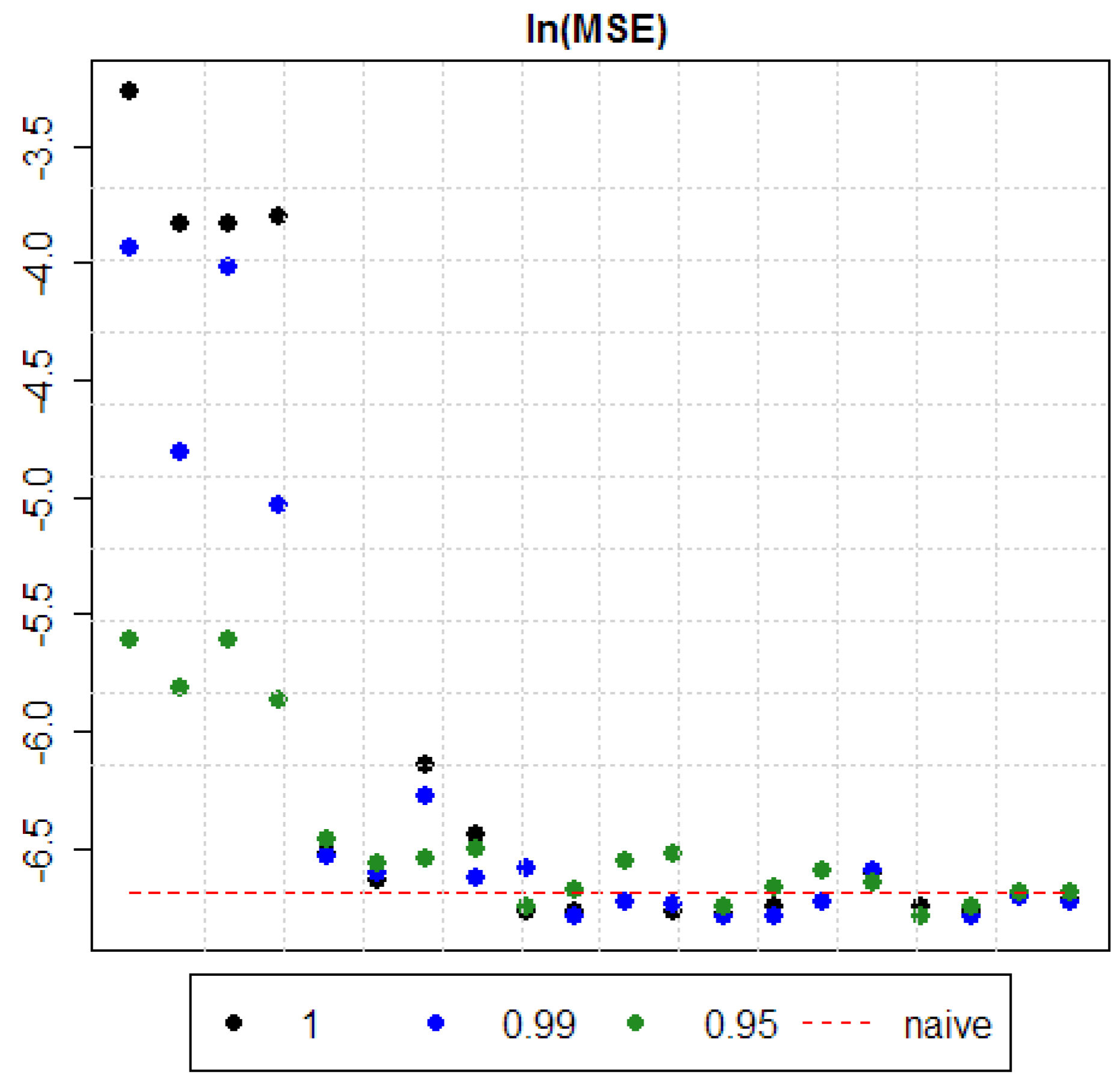
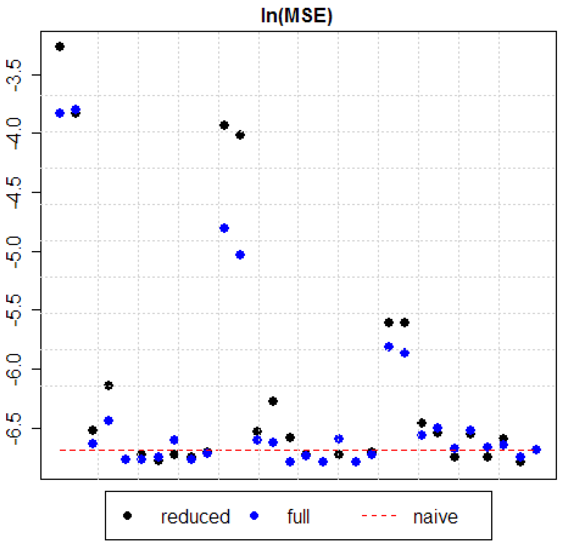
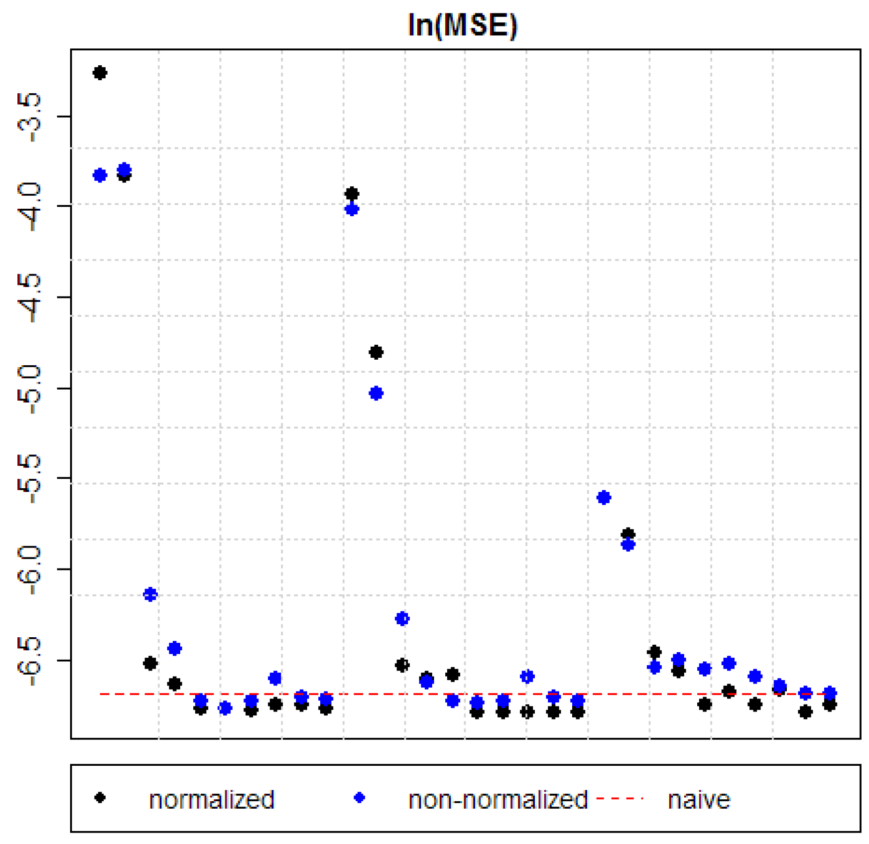
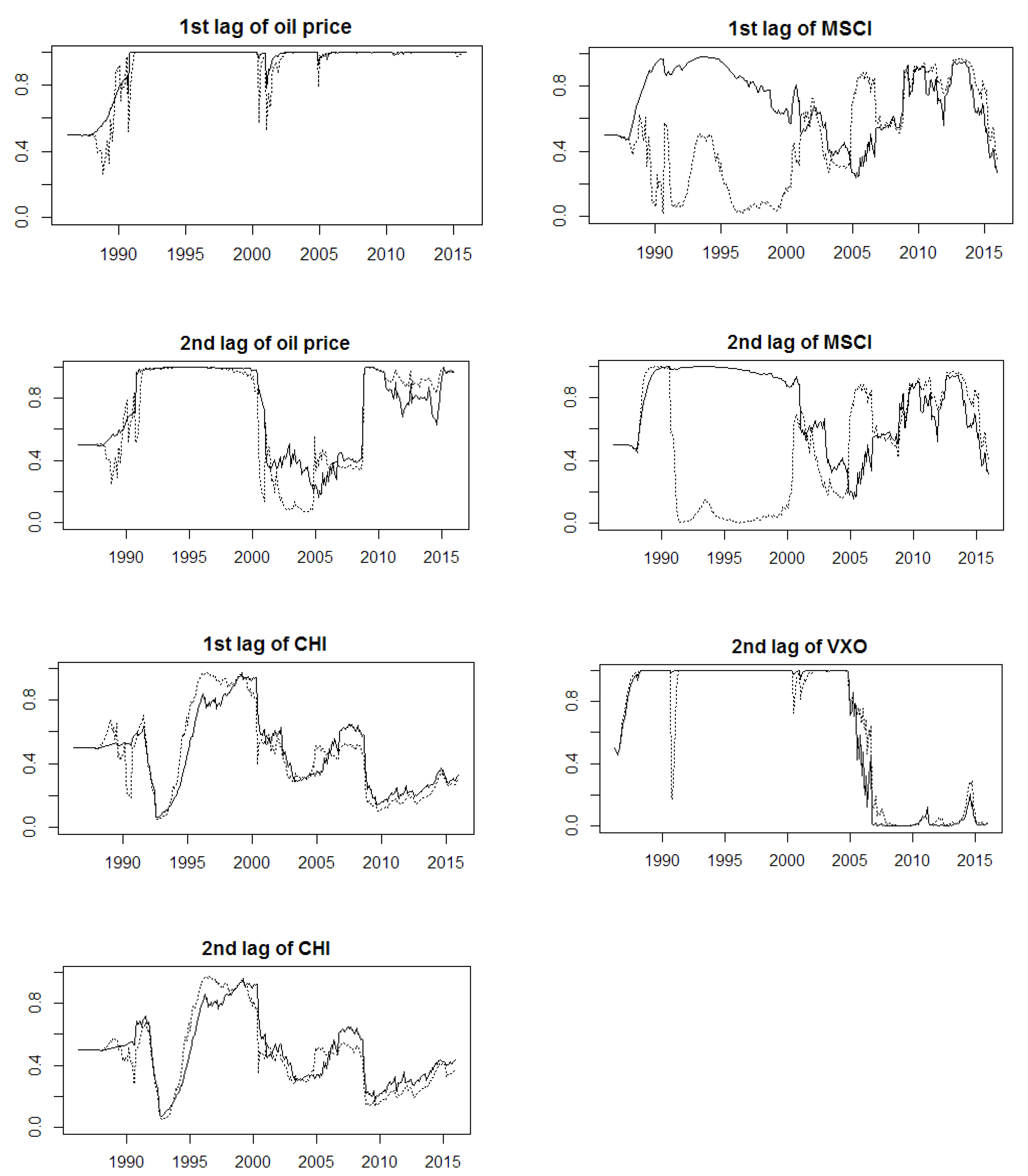
Table 1.
Description of time-series used.
| Name | Description | Economic Factor Measured by the Driver (and Units) |
|---|---|---|
| dependent variable in regression models | ||
| WTI | WTI spot price | crude oil spot price (in USD) |
| independent variables in regression models (drivers) | ||
| MSCI | MSCI World Index | stocks prices (index) |
| TB3MS | U.S. 3-month treasury bill secondary market rate | interest rate (in percentages) |
| KEI | Kilian’s index of global economy activity [101] | global economic activity (index) |
| TWEXM | trade weighted U.S. dollar index | exchange rate (Mar, 1973 = 100) |
| PROD | U.S. crude oil production | oil supply (in thousand barrels) |
| IMP | daily average of U.S. crude oil import | oil demand (in thousand barrels per day) |
| INV | U.S. total ending stocks of commercial crude oil (excluding SPR) | speculative pressures (in thousand barrels) |
| VXO | implied volatility of S&P 100 | volatility of stocks market (index) |
| CONS | total consumption of petroleum products in OECD | oil demand (in quad BTU) |
| CHI | Shanghai Composite Index merged with Hang Seng Index as a representative of Chinese economy | Chinese economy (rescaled index) |
| other time-series | ||
| NFP | 1-month NYMEX WTI futures prices | alternative forecast of crude oil price (in USD) |
Table 2.
Lists of drivers considered in the constructed DMA models.
| Model | xt(k) (Drivers Considered in the Model) |
|---|---|
| Model 1 | 1st lag of MSCI, |
| 1st lag of TB3MS, 1st lag of KEI, 1st lag of TWEXM, 1st lag of PROD, 1st lag of IMP,1st lag of INV, | |
| 1st lag of VXO, 1st lag of CONS, 1st lag of CHI | |
| Model 2 | 1st lag of WTI, |
| 1st lag of MSCI, | |
| 1st lag of TB3MS, 1st lag of KEI, 1st lag of TWEXM, 1st lag of PROD, 1st lag of IMP, 1st lag of INV, | |
| 1st lag of VXO, 1st lag of CONS, 1st lag of CHI | |
| Model 3 | 1st lag of WTI, |
| 1st lag of MSCI, | |
| 1st lag of TB3MS, 1st lag of KEI, 1st lag of TWEXM, 1st lag of PROD, 1st lag of IMP, 1st lag of INV, | |
| 1st lag of VXO, 1st lag of CONS, 1st lag of CHI, | |
| 1st lag of NFP | |
| Model 4 | 1st lag of WTI, 2nd lag of WTI, |
| 1st lag of MSCI, 2nd lag of MSCI, | |
| 1st lag of TB3MS, 1st lag of KEI, 1st lag of TWEXM, 1st lag of PROD, 1st lag of IMP, 1st lag of INV, | |
| 1st lag of VXO, 1st lag of CONS, 1st lag of CHI, | |
| Model 5 | 1st lag of WTI, 2nd lag of WTI, 1st lag of MSCI, 2nd lag of MSCI, 1st lag of VXO, 2nd lag of VXO, |
| 1st lag of CHI, 2nd lag of CHI |
Table 3.
“Reduced” models.
| Presence of the Driver in the Model with Normalized Data is Indicated by “x”, and in the Model with Non-Normalized Data by “o”. | |||||||||||||||
|---|---|---|---|---|---|---|---|---|---|---|---|---|---|---|---|
| Model 1 | Model 2 | Model 3 | Model 4 | Model 5 | |||||||||||
| α | 1 | 0.99 | 0.95 | 1 | 0.99 | 0.95 | 1 | 0.99 | 0.95 | 1 | 0.99 | 0.95 | 1 | 0.99 | 0.95 |
| 1st lag of WTI | x o | x o | x o | x o | x o | x o | x o | x o | x o | x o | x o | x o | |||
| 2nd lag of WTI | x o | x o | x o | x o | x o | x o | |||||||||
| 1st lag of MSCI | x o | x o | o | o | x o | x o | o | x o | |||||||
| 2nd lag of MSCI | x o | o | x o | ||||||||||||
| 1st lag of TB3MS | x | o | x o | x o | x | x o | x | x o | x o | x | x o | ||||
| 1st lag of KEI | x | x o | x o | x o | x | x o | |||||||||
| 1st lag of TWEXM | x o | x o | x o | x | x o | x | x | x o | x o | x | x o | ||||
| 1st lag of PROD | o | o | x | x o | x | x o | x | x | x o | ||||||
| 1st lag of IMP | x o | o | x | o | x | ||||||||||
| 1st lag of INV | x o | o | x | o | x | ||||||||||
| 1st lag of VXO | x | x o | o | x | o | o | o | o | x o | ||||||
| 2nd lag of VXO | x | x | x | ||||||||||||
| 1st lag of CONS | o | x | x o | x o | x | x o | x | x o | |||||||
| 1st lag of CHI | x | x | o | x | x o | ||||||||||
| 2nd lag of CHI | o | x o | x o | ||||||||||||
| 1st lag of NFP | x o | o | x o | ||||||||||||
Table 4.
MSE for estimated models.
| Models | α | |||
|---|---|---|---|---|
| 1 | 0.99 | 0.95 | ||
| Model 1 (normalized) | reduced | 0.03794 | 0.01949 | 0.00365 |
| full | 0.02169 | 0.00817 | 0.00298 | |
| Model 1 (non-normalized) | reduced | 0.02176 | 0.01795 | 0.00365 |
| full | 0.02235 | 0.00654 | 0.00283 | |
| Model 2 (normalized) | reduced | 0.00147 | 0.00145 | 0.00156 |
| full | 0.00131 | 0.00135 | 0.00141 | |
| Model 2 (non-normalized) | reduced | 0.00215 | 0.00187 | 0.00144 |
| full | 0.00159 | 0.00132 | 0.00150 | |
| Model 3 (normalized) | reduced | 0.00115 | 0.00138 | 0.00117 |
| full | 0.00115 | 0.00113 | 0.00126 | |
| Model 3 (non-normalized) | reduced | 0.00120 | 0.00120 | 0.00142 |
| full | 0.00115 | 0.00118 | 0.00147 | |
| Model 4 (normalized) | reduced | 0.00114 | 0.00112 | 0.00117 |
| full | 0.00117 | 0.00112 | 0.00127 | |
| Model 4 (non-normalized) | reduced | 0.00119 | 0.00120 | 0.00136 |
| full | 0.00135 | 0.00136 | 0.00130 | |
| Model 5 (normalized) | reduced | 0.00117 | 0.00113 | 0.00113 |
| full | 0.00115 | 0.00113 | 0.00117 | |
| Model 5 (non-normalized) | reduced | 0.00122 | 0.00122 | 0.00124 |
| full | 0.00121 | 0.00120 | 0.00125 | |
| Benchmarks | ||||
| 1-month futures | 0.00122 | |||
| naïve (i.e., the last period’s actuals are used as this period’s forecast) | 0.00124 | |||
| Equal-Weighted Averaging | 0.02694 | |||
| MSE smaller than those of benchmark forecasts are bolded. | ||||
Table 5.
Results of the Diebold-Mariano test for forecast accuracy.
| Halt: Forecast from the Chosen Model is More Accurate than the Forecast from the … | Stat. | p-val. |
|---|---|---|
| BMA | 0.8676 | 0.1931 |
| Equal-Weighted Averaging | 9.5349 | 0.0000 |
| 1-month futures | 0.7614 | 0.2235 |
| naive | 14.6047 | 0.0000 |
| Model 1 (normalized) | 8.7911 | 0.0000 |
| Model 2 (normalized) | 2.0940 | 0.0185 |
| Model 3 (normalized) | 1.8576 | 0.0320 |
| Model 4 (normalized) | −0.1078 | 0.5429 |
Table 6.
Comparison of investment strategies.
| Strategy | Mean | SD | Sharpe Ratio |
|---|---|---|---|
| DMA | 0.0069 | 0.0614 | 0.1131 |
| “Hold oil” | 0.0066 | 0.0848 | 0.0778 |
| Based on futures | −0.0010 | 0.0688 | −0.0141 |
© 2018 by the author. Licensee MDPI, Basel, Switzerland. This article is an open access article distributed under the terms and conditions of the Creative Commons Attribution (CC BY) license (http://creativecommons.org/licenses/by/4.0/).
Share and Cite
MDPI and ACS Style
Drachal, K. Determining Time-Varying Drivers of Spot Oil Price in a Dynamic Model Averaging Framework. Energies 2018, 11, 1207. https://doi.org/10.3390/en11051207
AMA Style
Drachal K. Determining Time-Varying Drivers of Spot Oil Price in a Dynamic Model Averaging Framework. Energies. 2018; 11(5):1207. https://doi.org/10.3390/en11051207
Chicago/Turabian StyleDrachal, Krzysztof. 2018. "Determining Time-Varying Drivers of Spot Oil Price in a Dynamic Model Averaging Framework" Energies 11, no. 5: 1207. https://doi.org/10.3390/en11051207
Note that from the first issue of 2016, this journal uses article numbers instead of page numbers. See further details here.