Nonlinear Modeling and Dynamic Analyses of the Hydro–Turbine Governing System in the Load Shedding Transient Regime

Abstract

Load shedding processes are widespread in hydropower stations, which has great influence on the safe and stable operation of the hydro–turbine governing system. In order to study the dynamic characteristics of the hydro–turbine governing system during the load shedding process, a novel nonlinear mathematical model of the hydro–turbine governing system is established considering the hydro–turbine system, the generator system and the governor system. In particular, a novel nonlinear mathematical model of the six hydro–turbine transfer coefficients is presented based on the definitions and hydro–turbine internal characteristics. After that, from the viewpoint of nonlinear dynamics and the practical engineering, the dynamic characteristics of the hydro–turbine governing system are investigated utilizing bifurcation diagrams, time series, Poincare maps, power spectrums and phase planes. Some meaningful results are found. The advantages of the novel nonlinear mathematical model are illustrated and commented in detail in comparison with the previous model. Finally, these models and analysis results will provide some theoretical references for the operation of hydropower stations in the load shedding transient.

1. Introduction

Hydraulic power, as a kind of renewable, clean, and economical resource, has been well developed in China [1,2,3]. By the end of 2015, the combined installed hydropower station capacity reached 320.03 GW [4,5]. However, some challenges are also found in the operation of the hydro–turbine generator units [6,7,8,9,10], such as water hammer in the penstock, the self–oscillation of the machinery, the unbalanced magnetic pull, and so on. At the same time, with the rapid development of wind energy and the photovoltaic power generation in recent years, these unstable resources need to be balanced utilizing hydropower stations [11,12,13,14]. All these factors could increase the instability of the whole hydro–turbine generator system, especially, the hydro–turbine governing system (HTGS). Therefore, to ensure the safe and stable operation of the hydro–turbine generator unit, the study of the dynamic characteristics of the HTGS is necessary.

The transient process of the HTGS mainly comprises the major fluctuation processes and the small fluctuation processes. In the previous studies, much attention has been paid to the small fluctuation processes [15,16,17,18,19,20,21,22,23]. Many scholars have proposed excellent control algorithms [15,16,17,18,19,20] to adjust the hydro–turbine generator unit when some small disturbances appear, or established reasonable models to study the stability and other dynamic characteristics of the HTGS during the small fluctuation process [21,22,23]. Chang et al. [15] proposed a kind of effective neural–network–predict–control method to optimizing the control of the HTGS. Based on the polynomial robust H_∞ optimization method, Eker [16] presented a robust single–input multi–output design approach for governors for speed control of hydro–turbines. Khodabakhshian and Hooshmand [17] put forward a new robust proportional-integral-derivative (PID) controller for automatic generation control of hydro–turbine power systems, which is designed mainly based on a maximum peak resonance specification. Ren et al. [18] proposed an improved cascade control strategy for hydro–turbine speed governors, which can effectively decrease fluctuations of the rotational speed under non–Gaussian disturbance conditions in practical hydropower plants. Chen et al. [19] focused on designing the fractional–order PID controller using a chaotic non–dominated sorting genetic algorithm II for the HTGS, which has a better performance than traditional integer PID controllers. Zhang et al. [20] created a brand new non–linear predictive control method using the Takagi–Sugeno (T–S) fuzzy method and the generalized predictive control, which can govern a non–linear system more effectively. Chen et al. [21] established a new nonlinear mathematical model of the HTGS with a surge tank, and then, the nonlinear dynamical behaviors of the system in small fluctuation process were studied in detail. Guo et al. [22] studied the stability of the HTGS of the hydropower station with sloping ceiling tailrace tunnel utilizing the Hopf bifurcation theory, and also got the algebraic criterion of the occurrence of Hopf bifurcation. Xu et al. [23] built the Hamiltonian mathematical model of the multi–hydro–turbine governing system with a sharing common penstock under the excitation of stochastic and shock load, and then, discussed the stability of the system by comparing it with a real hydropower station. In these studies, constant or linear hydro–turbine transfer coefficients are mainly applied to.

Regarding the major fluctuation process, many published papers [24,25,26,27,28] mainly adopt a simple nonlinear model to analyze the dynamic characteristics of the HTGS during the major fluctuation, in which some linear or approximate nonlinear hydro–turbine transfer coefficient models are widely applied. However, when the hydro–turbine generator unit undergoes a major fluctuation process, the dynamic characteristics of the hydro–turbine generator unit are very complex, including hydraulic [6,8], electrical [26], and mechanical instability [29,30], so the hydro–turbine transfer coefficients expressed by the constant value, the linear model or the approximate nonlinear model could lead to unreasonable, and even wrong results. In light of the foregoing analyses, previous simple models cannot meet the needs of scientific researches and engineering practices, a more reasonable model needs to be established to describe the dynamic characteristics of the HTGS in the major fluctuation process.

Motivated by the above discussions, there are three advantages that make our research more attractive. First, the six hydro–turbine transfer coefficients are calculated more accurately based on definitions and hydro–turbine internal characteristics, which are appropriate for nonlinear dynamic studies of the HTGS in the major fluctuation. Second, a novel nonlinear mathematical model of the HTGS in the load shedding transient process is established with the elastic water hammer model of the penstock. Finally, the nonlinear dynamic characteristics of the HTGS are studied in detail, and some meaningful results are also presented. The rest of the paper is organized as follows: in Section 2, the mathematical model of the HTGS is established. Section 3 analyzes the nonlinear dynamic characters of the system. Section 4 closes the paper.

2. Mathematical Model of the Hydro–Turbine Governing System

2.1. Mathematical Model of the Francis Hydro–Turbine

The structure of the Francis HTGS [24] is usually described as shown in Figure 1.

The dynamic characteristics of the Francis hydro–turbine [21,22,23,24] can be expressed as:

$$\{\begin{array}{l}{M}_t=M_t(H,W,Y)\\ Q=Q(H,W,Y)\end{array},$$

(1)

where M_t, Q, H, W and Y are the mechanical torque of the hydro–turbine, the hydro–turbine flow, the hydro–turbine head, the rotational speed and the guide vane opening, respectively. For convenience, the relative deviation values of them are denoted by m_t, q, h, ω and y, respectively, and the corresponding relative values ($m_t^{*}$, $q^{*}$, $h^{*}$, ${\omega }^{*}$ and $y^{*}$) are marked by the superscript (*). Then, m_t and q can be written as:

$$\{\begin{array}{l}{m}_t=e_{my}y+e_{mh}h+e_{m\omega }\omega \\ q=e_{qy}y+e_{qh}h+e_{q\omega }\omega \end{array},$$

(2)

where e_my, e_mh, and e_mω are transfer coefficients of the hydro–turbine torque (m_t) with respect to the guide vane opening (y), the hydro–turbine head (h), and the rotational speed (ω), respectively. e_qy, e_qh and e_qω, respectively, denote transfer coefficients of the hydro–turbine flow (q) with respect to the guide vane opening (y), the hydro–turbine head (h), and the rotational speed (ω). Thus, these six hydro–turbine transfer coefficients can be calculated by $e_{my}=(\partial m_t/\partial y)$, $e_{mh}=(\partial m_t/\partial h)$, $e_{m\omega }=(\partial m_t/\partial \omega )$, $e_{qy}=(\partial q/\partial y)$, $e_{qh}=(\partial q/\partial h)$, and $e_{q\omega }=(\partial q/\partial \omega )$.

2.2. Dynamic Characteristics of the Penstock System

For simplifying the calculation, the elasticity of the water and pipes are usually ignored in the modeling of the small fluctuation process for the penstock system, and a rigid water hammer model is applied to. However, for the major fluctuation, the rigid hammer model cannot meet requirements of the engineering, the influence of the elasticity of the water and pipes must be considered.

From [23,31], the transfer function of the penstock system with elastic water hammer can be written as:

$$G_h(s)=\frac{H(s)}{Q(s)}=-2h_w\frac{sh(\frac{T_r}{2}s)}{ch(\frac{T_r}{2}s)}\approx -2h_w\frac{\frac{1}{48}{T}_r^3{s}^3+\frac{1}{2}{T}_{r}s}{\frac{1}{8}{T}_r^2{s}^2+1},$$

(3)

where h_w is a coefficient describing the pipe characteristic, T_r is the elastic hammer time constant.

Thus, the state–space equations of Equation (3) can be expressed as:

$$\{\begin{array}{l}{\dot{x}}_1=x_2\\ {\dot{x}}_2=x_3\\ {\dot{x}}_3=-a_1{x}_2+h\\ \dot{q}=b_1{x}_2-a_1{b}_2{x}_2+b_{2}h\end{array},\mathrm{overlapping}\mathrm{symbols}$$

(4)

where $a_1=24/T_r^2$, $b_1=-24/(h_w{T}_r^3)$ and $b_2=-3/(h_w{T}_r)$. x₁, x₂ and x₃ are intermediate variables.

2.3. Mathematical Model of the Generator

A second–order generator model [31] is considered, which can be written as:

$$\{\begin{array}{l}\dot{\delta }={\omega }_B\omega \\ \dot{\omega }=\frac{1}{T_{ab}}\left(m_t-m_e-D\omega \right)\end{array},$$

(5)

where $\delta$ is the rotor angle, m_e is the relative deviation of the electromagnetic torque, T_ab is the mechanical starting time, D is the damping coefficient, ω_B = 2πf₀ and f₀ = 50 Hz.

According to generator dynamic characteristics, if the change of the electromagnetic torque caused by rotational speed is included in damping coefficient, the electromagnetic torque (m_e) will be equal to its electromagnetic power (P_e) [31]. Therefore, it can be written as:

$$m_e=P_e.$$

(6)

The electromagnetic power of the salient pole hydro–turbine generator can be expressed as:

$$P_e=\frac{E_q^{\prime }{V}_s}{x_{d\mathrm{\Sigma }}^{\prime }}\sin \delta +\frac{V_s^2}{2}\frac{x_{d\mathrm{\Sigma }}^{\prime }-x_{q\mathrm{\Sigma }}}{x_{d\mathrm{\Sigma }}^{\prime }{x}_{q\mathrm{\Sigma }}}\sin 2\delta ,$$

(7)

where $E_q^{\prime }$ is the transient electric potential of the generator q-axis, $V_s$ is the busbar voltage, $x_d^{\prime }$ is the transient reactance of the generator d-axis, $x_q$ is the synchronous reactance of the generator q-axis. Besides, $x_{d\mathrm{\Sigma }}^{\prime }$ and $x_{q\Sigma }$ can be calculated by:

$$\{\begin{array}{l}{x}_{d\mathrm{\Sigma }}^{\prime }={\dot{x}}_d+x_T+\frac{1}{2}{x}_L\\ x_{q\mathrm{\Sigma }}=x_q+x_T+\frac{1}{2}{x}_L\end{array},$$

(8)

where $x_T$ is the short–circuit reactance of the transformer, $x_L$ is the reactance of the electric transmission line.

Therefore, combining Equations (5)–(8), the generator model can be written as:

$$\{\begin{array}{l}\dot{\delta }={\omega }_B\omega \\ \dot{\omega }=\frac{1}{T_{ab}}\left(m_t-\frac{E_q^{\prime }{V}_s}{x_{d\mathrm{\Sigma }}^{\prime }}\sin \delta -\frac{V_s^2}{2}\frac{x_{d\mathrm{\Sigma }}^{\prime }-x_{q\mathrm{\Sigma }}}{x_{d\mathrm{\Sigma }}^{\prime }{x}_{q\mathrm{\Sigma }}}\sin 2\delta -D\omega \right)\end{array}$$

(9)

2.4. Mathematical Model of the Hydraulic Speed Regulation System

The parallel PID governor is wildly applied in many hydropower stations. Its regulator output u can be expressed as:

$$u=-k_p\omega -k_i{\displaystyle {\int }_0^t\omega dt}-k_d\dot{\omega }=-k_p\omega -\frac{k_i}{{\omega }_B}\delta -k_d\dot{\omega },$$

(10)

where k_p, k_i, and k_d denote the proportional, integral, and differential adjustment coefficient, respectively.

The dynamic characteristic of the hydraulic servo system can be described as:

$$T_y\frac{dy}{dt}+y=u,$$

(11)

where $T_y$ is the response time of the servomotor.

Combining Equations (9) and (10), Equation (12) can be obtained:

$$\dot{y}=\frac{1}{T_y}(-k_p\omega -\frac{k_i}{{\omega }_B}\delta -k_d\dot{\omega }-y).$$

(12)

2.5. Nonlinear Expressions of the Hydro–Turbine Transfer Coefficients

When the hydro–turbine generator unit operates under small fluctuation conditions, the transfer coefficients of the hydro–turbine are usually calculated by the constant transfer coefficient method [31], the simple linear method [26], or the external characteristic method [32]. However, the simple linear method and the constant transfer coefficient method only apply to the small fluctuation condition. At the same time, the external characteristic method cannot describe hydro–turbine characteristics in the poor efficiency region, so the external characteristic method also loses efficacy when the hydro–turbine generator unit operates under major fluctuation conditions. Therefore, in this paper, the internal characteristic method will be used to calculate hydro–turbine transfer coefficients according to their definitions.

For the Francis hydro–turbine, internal characteristic equations [33] can be written as:

$$Q=\frac{W{r}^2+\frac{9.8\eta H}{W}}{\frac{\cot \alpha }{2\pi b_0}+r\frac{\cot {\beta }_0}{A}}$$

(13)

and:

$$M_t=Q[(\frac{\cot \alpha }{2\pi b_0}+r\frac{\cot {\beta }_0}{A})Q-W{r}^2],$$

(14)

where $\alpha$ is the guide vane discharge angle, b₀ is the height of the guide vane, $\eta$ is the efficiency of the hydro–turbine, A is the runner outlet area, r is the radius of the runner intermediate flow surface and ${\beta }_0$ is the runner intermediate flow surface angle.

Combining Equations (12) and (13), and replacing M_t, W, H and Q by corresponding relative values ($m_t^{*}$, ${\omega }^{*}$, $h^{*}$, $q^{*}$), it can be gotten:

$$M_{tr}{m}_t^{*}-\left(\frac{\cot \alpha }{2\pi b_0}+r\frac{\cot {\beta }_0}{A}\right){\left[\frac{W_r{\omega }^{*}{r}^2+\frac{9.8\eta H_r{h}^{*}}{W_r{\omega }^{*}}}{\frac{\cot \alpha }{2\pi b_0}+r\frac{\cot {\beta }_0}{A}}\right]}^2-W_r{\omega }^{*}{r}^2\left[\frac{W_r{\omega }^{*}{r}^2+\frac{9.8\eta H_r{h}^{*}}{W_r{\omega }^{*}}}{\frac{\cot \alpha }{2\pi b_0}+r\frac{\cot {\beta }_0}{A}}\right]=0.$$

(15)

The relationship between guide vane opening (Y) and the guide vane discharge angle ($\alpha$) can be written as:

$$Y=D_0\sin (\frac{\beta }{2})\sin (\alpha +\frac{\beta }{2})-L\sin (\frac{\beta }{2}),$$

(16)

where D₀ is the distribution circle diameter, L is the guide vane width, $\beta$ is the width between two guide vanes.

Replacing the guide vane opening (Y) in Equation (15) with corresponding relative value ($y^{*}$), the guide vane discharge angle ($\alpha$) can be expressed as:

$$\alpha =\arcsin \left[\frac{Y_r{y}^{*}+L\sin (\frac{\beta }{2})}{D_0\sin (\frac{\beta }{2})}\right]-\frac{\beta }{2}.$$

(17)

Therefore:

$$\frac{\partial \alpha }{\partial y^{*}}=\frac{1}{\sqrt{1-{\left(\frac{Y_r{y}^{*}+L\sin (\frac{\beta }{2})}{D_0\sin (\frac{\beta }{2})}\right)}^{{}^2}}}\cdot Y_r.$$

(18)

Define a function $F_1(m_t^{*},\alpha ,h^{*},{\omega }^{*})$ according to Equation (14), it can be expressed as:

$$F_1(m_t^{*},\alpha ,h^{*},{\omega }^{*})=M_{tr}{m}_t^{*}-\left(\frac{\cot \alpha }{2\pi b_0}+r\frac{\cot {\beta }_0}{A}\right){\left[\frac{W_r{\omega }^{*}{r}^2+\frac{9.8\eta H_r{h}^{*}}{W_r{\omega }^{*}}}{\frac{\cot \alpha }{2\pi b_0}+r\frac{\cot {\beta }_0}{A}}\right]}^2-W_r{\omega }^{*}{r}^2\left[\frac{W_r{\omega }^{*}{r}^2+\frac{9.8\eta H_r{h}^{*}}{W_r{\omega }^{*}}}{\frac{\cot \alpha }{2\pi b_0}+r\frac{\cot {\beta }_0}{A}}\right].$$

(19)

Then according to Equation (18), the partial derivative of the hydro–turbine torque ($m_t^{*}$) with respect to the guide vane discharge angle ($\alpha$) can be expressed as:

$$\frac{\partial m_t^{*}}{\partial \alpha }=-\frac{\frac{\partial F_1}{\partial \alpha }}{\frac{\partial F_1}{\partial m_t^{*}}}=\frac{1}{M_{tr}}\cdot \frac{1}{{\left(\frac{\cot \alpha }{2\pi b_0}+r\frac{\cot {\beta }_0}{A}\right)}^2}\cdot \frac{{\csc }^2\alpha }{2\pi b_0}\cdot \left[\left(2W_r{\omega }^{*}{r}^2+\frac{9.8\eta H_r{h}^{*}}{W_r{\omega }^{*}}\right)\cdot \left(W_r{\omega }^{*}{r}^2+\frac{9.8\eta H_r{h}^{*}}{W_r{\omega }^{*}}\right)\right].$$

(20)

Thus, e_my, e_mh and e_mω can be calculated as:

$$\begin{array}{ll}{e}_{my}& =\frac{\partial m_t}{\partial y}=\frac{\partial (m_t^{*}-1)}{\partial (y^{*}-1)}=\frac{\partial (m_t^{*}-1)}{\partial y^{*}}\cdot \frac{\partial y^{*}}{\partial (y^{*}-1)}=\frac{\partial m_t^{*}}{\partial y^{*}}\cdot \frac{\partial y^{*}}{\partial (y^{*}-1)}=\frac{\partial m_t^{*}}{\partial y^{*}}=\frac{\partial m_t^{*}}{\partial \alpha }\cdot \frac{\partial \alpha }{\partial y^{*}}\\ & =\frac{1}{M_{tr}}\cdot \frac{1}{{\left(\frac{\cot \alpha }{2\pi b_0}+r\frac{\cot {\beta }_0}{A}\right)}^2}\cdot \frac{{\csc }^2\alpha }{2\pi b_0}\cdot \frac{Y_r}{\sqrt{1-{\left(\frac{Y_r(y+1)+L\sin (\frac{\beta }{2})}{D_0\sin (\frac{\beta }{2})}\right)}^{{}^2}}}\\ & \times \left[\left(2W_r(\omega +1)r^2+\frac{9.8\eta H_r(h+1)}{W_r(\omega +1)}\right)\cdot \left(W_r(\omega +1)r^2+\frac{9.8\eta H_r(h+1)}{W_r(\omega +1)}\right)\right]\end{array},$$

(21)

$$\begin{array}{ll}{e}_{mh}& =\frac{\partial m_t}{\partial h}=\frac{\partial (m_t^{*}-1)}{\partial (h^{*}-1)}=\frac{\partial (m_t^{*}-1)}{\partial h^{*}}\cdot \frac{\partial h^{*}}{\partial (h^{*}-1)}=\frac{\partial m_t^{*}}{\partial h^{*}}\cdot \frac{\partial h^{*}}{\partial (h^{*}-1)}=\frac{\partial m_t^{*}}{\partial h^{*}}\\ & =-\frac{\frac{\partial F_1}{\partial h^{*}}}{\frac{\partial F_1}{\partial m_t^{*}}}=\frac{1}{M_{tr}}\cdot \frac{1}{\frac{\cot \alpha }{2\pi b_0}+r\frac{\cot {\beta }_0}{A}}\cdot \left[2(h+1)\cdot {\left(\frac{9.8\eta H_r}{W_r(\omega +1)}\right)}^2+3\times 9.8\eta H_r{r}^2\right]\end{array},$$

(22)

and:

$$\begin{array}{ll}{e}_{m\omega }& =\frac{\partial m_t}{\partial \omega }=\frac{\partial (m_t^{*}-1)}{\partial ({\omega }^{*}-1)}=\frac{\partial (m_t^{*}-1)}{\partial {\omega }^{*}}\cdot \frac{\partial {\omega }^{*}}{\partial ({\omega }^{*}-1)}=\frac{\partial m_t^{*}}{\partial {\omega }^{*}}\cdot \frac{\partial {\omega }^{*}}{\partial ({\omega }^{*}-1)}=\frac{\partial m_t^{*}}{\partial {\omega }^{*}}\\ & =-\frac{\frac{\partial F_1}{\partial {\omega }^{*}}}{\frac{\partial F_1}{\partial m_t^{*}}}=\frac{1}{M_{tr}}\cdot \frac{1}{\frac{\cot \alpha }{2\pi b_0}+r\frac{\cot {\beta }_0}{A}}\cdot \left\{2(\omega +1)\left[{\left(W_r{r}^2\right)}^2-{\left(\frac{9.8\eta H_r(h+1)}{W_r{(\omega +1)}^2}\right)}^2\right]+2W_r^2{r}^4(\omega +1)\right\}\end{array}.$$

(23)

Equation (13) can also be written as:

$$M_{tr}{m}_t^{*}-Q_r{q}^{*}[(\frac{\cot \alpha }{2\pi b_0}+r\frac{\cot {\beta }_0}{A})Q_r{q}^{*}-W_r{\omega }^{*}{r}^2]=0.$$

(24)

Define a function $F_2(q^{*},m_t^{*},\alpha ,h^{*},{\omega }^{*})$ according to Equation (23), it can be written as:

$$F_2(q^{*},m_t^{*},\alpha ,h^{*},{\omega }^{*})=M_{tr}{m}_t^{*}-Q_r{q}^{*}[(\frac{\cot \alpha }{2\pi b_0}+r\frac{\cot {\beta }_0}{A})Q_r{q}^{*}-W_r{\omega }^{*}{r}^2].$$

(25)

Then $\partial q^{*}/\partial m_t^{*}$ can be calculated as:

$$\frac{\partial q^{*}}{\partial m_t^{*}}=-\frac{\frac{\partial F_2}{\partial m_t^{*}}}{\frac{\partial F_2}{\partial q^{*}}}=-\frac{M_{tr}}{-2Q_r^2\left(\frac{\cot \alpha }{2\pi b_0}+r\frac{\cot {\beta }_0}{A}\right)q^{*}+W_r{r}^2{Q}_r{\omega }^{*}}.$$

(26)

Thus, e_qy, e_qh and e_qω can be calculated as:

$$e_{qy}=\frac{\partial q}{\partial y}=\frac{\partial q^{*}}{\partial y^{*}}=\frac{\partial q^{*}}{\partial m_t^{*}}\cdot \frac{\partial m_t^{*}}{\partial y^{*}}=-\frac{M_{tr}}{-2Q_r^2\left(\frac{\cot \alpha }{2\pi b_0}+r\frac{\cot {\beta }_0}{A}\right)\cdot (q+1)+W_r{r}^2{Q}_r(\omega +1)}\cdot e_{my},$$

(27)

$$e_{qh}=\frac{\partial q}{\partial h}=\frac{\partial q^{*}}{\partial h^{*}}=\frac{\partial q^{*}}{\partial m_t^{*}}\cdot \frac{\partial m_t^{*}}{\partial h^{*}}=-\frac{M_{tr}}{-2Q_r^2\left(\frac{\cot \alpha }{2\pi b_0}+r\frac{\cot {\beta }_0}{A}\right)\cdot (q+1)+W_r{r}^2{Q}_r(\omega +1)}\cdot e_{mh}$$

(28)

and:

$$e_{q\omega }=\frac{\partial q}{\partial \omega }=\frac{\partial q^{*}}{\partial {\omega }^{*}}=\frac{\partial q^{*}}{\partial m_t^{*}}\cdot \frac{\partial m_t^{*}}{\partial {\omega }^{*}}=-\frac{M_{tr}}{-2Q_r^2\left(\frac{\cot \alpha }{2\pi b_0}+r\frac{\cot {\beta }_0}{A}\right)\cdot (q+1)+W_r{r}^2{Q}_r(\omega +1)}\cdot e_{m\omega }.$$

(29)

For analyzing the dynamic characteristics of the HTGS in the load shedding transient, a typical major fluctuation process, the closing time of the guide vane is set for 3 s based on [24]. The closing rule is shown in Figure 2. Besides, assuming the full load is rejected.

2.6. Mathematical Model of the Hydro–Turbine Governing System

Combining Equations (2), (20)–(22), the hydro–turbine torque characteristic can be expressed as:

$$\begin{array}{ll}{\dot{m}}_t& =\frac{1}{M_{tr}}\cdot \left[\frac{\left(2W_r(\omega +1)r^2+\frac{9.8\eta H_r(h+1)}{W_r(\omega +1)}\right)\cdot \left(W_r(\omega +1)r^2+\frac{9.8\eta H_r(h+1)}{W_r(\omega +1)}\right)}{{\left(\frac{\cot \alpha }{2\pi b_0}+r\frac{\cot {\beta }_0}{A}\right)}^2}\cdot \frac{{\csc }^2\alpha }{2\pi b_0}\right]\cdot \frac{Y_r}{\sqrt{1-{\left(\frac{Y_r(y+1)+L\sin (\frac{\beta }{2})}{D_0\sin (\frac{\beta }{2})}\right)}^{{}^2}}}\cdot \dot{y}\\ & +\frac{1}{M_{tr}}\cdot \frac{1}{\frac{\cot \alpha }{2\pi b_0}+r\frac{\cot {\beta }_0}{A}}\cdot \left[2\left(2W_r(\omega +1)r^2+\frac{9.8\eta H_r(h+1)}{W_r(\omega +1)}\right)\cdot \frac{9.8\eta H_r}{W_r(\omega +1)}\right]\cdot \dot{h}\\ & +\frac{1}{M_{tr}}\cdot \frac{1}{\frac{\cot \alpha }{2\pi b_0}+r\frac{\cot {\beta }_0}{A}}\cdot \left[2\left(W_r(\omega +1)r^2+\frac{9.8\eta H_r(h+1)}{W_r(\omega +1)}\right)\cdot \left(W_r{r}^2-\frac{9.8\eta H_r(h+1)}{W_r{(\omega +1)}^2}\right)+2W_r^2{r}^4(\omega +1)\right]\cdot \dot{\omega }\end{array}.$$

(30)

According to Equation (2), the hydro–turbine head can be described as:

$$\dot{h}=\frac{1}{e_{qh}}\left(\dot{q}-e_{qy}\dot{y}-e_{q\omega }\dot{\omega }\right).$$

(31)

Then, combining Equations (21)–(23), (27)–(29) and (31), we can obtain:

$$\dot{h}=\frac{\left[-2Q_r^2\left(\frac{\cot \alpha }{2\pi b_0}+r\frac{\cot {\beta }_0}{A}\right)\cdot (q+1)+W_r{r}^2{Q}_r(\omega +1)\right]\cdot \left(\frac{\cot \alpha }{2\pi b_0}+r\frac{\cot {\beta }_0}{A}\right)}{-\left[2(h+1)\cdot {\left(\frac{9.8\eta H_r}{W_r(\omega +1)}\right)}^2+3\times 9.8\eta H_r{r}^2\right]}\times \left\{\begin{array}{l}\frac{\left[\left(W_r(\omega +1)r^2+\frac{9.8\eta H_r(h+1)}{W_r(\omega +1)}\right)\cdot \left(W_r{r}^2-\frac{9.8\eta H_r(h+1)}{W_r{(\omega +1)}^2}\right)+W_r^2{r}^4(\omega +1)\right]}{-2Q_r^2\left(\frac{\cot \alpha }{2\pi b_0}+r\frac{\cot {\beta }_0}{A}\right)\cdot (q+1)+W_r{r}^2{Q}_r(\omega +1)}\cdot \frac{2\dot{\omega }}{\frac{\cot \alpha }{2\pi b_0}+r\frac{\cot {\beta }_0}{A}}\\ +\frac{\left[\left(2W_r(\omega +1)r^2+\frac{9.8\eta H_r(h+1)}{W_r(\omega +1)}\right)\cdot \left(W_r(\omega +1)r^2+\frac{9.8\eta H_r(h+1)}{W_r(\omega +1)}\right)\right]}{-2Q_r^2\left(\frac{\cot \alpha }{2\pi b_0}+r\frac{\cot {\beta }_0}{A}\right)\cdot (q+1)+W_r{r}^2{Q}_r(\omega +1)}\times \\ \frac{{\csc }^2\alpha }{2\pi b_0{\left(\frac{\cot \alpha }{2\pi b_0}+r\frac{\cot {\beta }_0}{A}\right)}^2}\cdot \frac{Y_r\dot{y}}{\sqrt{1-{\left(\frac{Y_r(y+1)+L\sin (\frac{\beta }{2})}{D_0\sin (\frac{\beta }{2})}\right)}^{{}^2}}}+\left(\frac{24}{h_w{T}_r^3}-\frac{72}{h_w{T}_r{T}_r^2}\right)x_2-\frac{3}{h_w{T}_r}h\end{array}\right\}.$$

(32)

In the end, based on Equations (4), (9), (12), (30) and (32), state–space equations of the HTGS in the load rejection transient can be expressed as:

$$\{\begin{array}{ll}{\dot{x}}_1& =x_2\\ {\dot{x}}_2& =x_3\\ {\dot{x}}_3& =-\frac{24}{T_r^2}{x}_2+h\\ \dot{\delta }& ={\omega }_B\omega \\ \dot{\omega }& =\frac{1}{T_{ab}}\left(m_t-\frac{E_q^{\prime }{V}_s}{x_{d\mathrm{\Sigma }}^{\prime }}\sin \delta -\frac{V_s^2}{2}\frac{x_{d\mathrm{\Sigma }}^{\prime }-x_{q\mathrm{\Sigma }}}{x_{d\mathrm{\Sigma }}^{\prime }{x}_{q\mathrm{\Sigma }}}\sin 2\delta -D\omega \right)\\ \dot{y}& =\frac{1}{T_y}(-k_p\omega -\frac{k_i}{{\omega }_B}\delta -k_d\dot{\omega }-y)\\ \dot{h}& =\frac{\left[-2Q_r^2\left(\frac{\cot \alpha }{2\pi b_0}+r\frac{\cot {\beta }_0}{A}\right)\cdot (q+1)+W_r{r}^2{Q}_r(\omega +1)\right]\cdot \left(\frac{\cot \alpha }{2\pi b_0}+r\frac{\cot {\beta }_0}{A}\right)}{-\left[2(h+1)\cdot {\left(\frac{9.8\eta H_r}{W_r(\omega +1)}\right)}^2+3\times 9.8\eta H_r{r}^2\right]}\times \left\{\begin{array}{l}\frac{\left[\left(W_r(\omega +1)r^2+\frac{9.8\eta H_r(h+1)}{W_r(\omega +1)}\right)\cdot \left(W_r{r}^2-\frac{9.8\eta H_r(h+1)}{W_r{(\omega +1)}^2}\right)+W_r^2{r}^4(\omega +1)\right]}{-2Q_r^2\left(\frac{\cot \alpha }{2\pi b_0}+r\frac{\cot {\beta }_0}{A}\right)\cdot (q+1)+W_r{r}^2{Q}_r(\omega +1)}\cdot \frac{2\dot{\omega }}{\frac{\cot \alpha }{2\pi b_0}+r\frac{\cot {\beta }_0}{A}}\\ +\frac{\left[\left(2W_r(\omega +1)r^2+\frac{9.8\eta H_r(h+1)}{W_r(\omega +1)}\right)\cdot \left(W_r(\omega +1)r^2+\frac{9.8\eta H_r(h+1)}{W_r(\omega +1)}\right)\right]}{-2Q_r^2\left(\frac{\cot \alpha }{2\pi b_0}+r\frac{\cot {\beta }_0}{A}\right)\cdot (q+1)+W_r{r}^2{Q}_r(\omega +1)}\times \\ \frac{{\csc }^2\alpha }{2\pi b_0{\left(\frac{\cot \alpha }{2\pi b_0}+r\frac{\cot {\beta }_0}{A}\right)}^2}\cdot \frac{Y_r\dot{y}}{\sqrt{1-{\left(\frac{Y_r(y+1)+L\sin (\frac{\beta }{2})}{D_0\sin (\frac{\beta }{2})}\right)}^{{}^2}}}+\left(\frac{24}{h_w{T}_r^3}-\frac{72}{h_w{T}_r{T}_r^2}\right)x_2-\frac{3}{h_w{T}_r}h\end{array}\right\}\\ \dot{q}& =\frac{-24}{h_w{T}_r^3}{x}_2+\frac{72}{h_w{T}_r{T}_r^2}{x}_2-\frac{3}{h_w{T}_r}h\\ {\dot{m}}_t& =\frac{1}{M_{tr}}\cdot \left[\frac{\left(2W_r(\omega +1)r^2+\frac{9.8\eta H_r(h+1)}{W_r(\omega +1)}\right)\cdot \left(W_r(\omega +1)r^2+\frac{9.8\eta H_r(h+1)}{W_r(\omega +1)}\right)}{{\left(\frac{\cot \alpha }{2\pi b_0}+r\frac{\cot {\beta }_0}{A}\right)}^2}\cdot \frac{{\csc }^2\alpha }{2\pi b_0}\right]\cdot \frac{Y_r}{\sqrt{1-{\left(\frac{Y_r(y+1)+L\sin (\frac{\beta }{2})}{D_0\sin (\frac{\beta }{2})}\right)}^{{}^2}}}\cdot \dot{y}\\ & +\frac{1}{M_{tr}}\cdot \frac{1}{\frac{\cot \alpha }{2\pi b_0}+r\frac{\cot {\beta }_0}{A}}\cdot \left[2\left(2W_r(\omega +1)r^2+\frac{9.8\eta H_r(h+1)}{W_r(\omega +1)}\right)\cdot \frac{9.8\eta H_r}{W_r(\omega +1)}\right]\cdot \dot{h}\\ & +\frac{1}{M_{tr}}\cdot \frac{1}{\frac{\cot \alpha }{2\pi b_0}+r\frac{\cot {\beta }_0}{A}}\cdot \left[2\left(W_r(\omega +1)r^2+\frac{9.8\eta H_r(h+1)}{W_r(\omega +1)}\right)\cdot \left(W_r{r}^2-\frac{9.8\eta H_r(h+1)}{W_r{(\omega +1)}^2}\right)+2W_r^2{r}^4(\omega +1)\right]\cdot \dot{\omega }\end{array}.$$

(33)

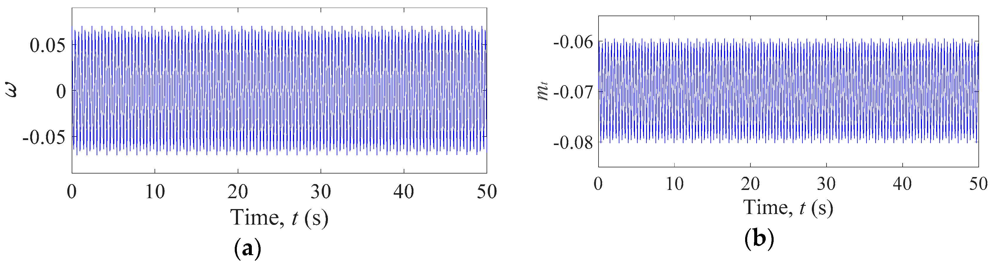
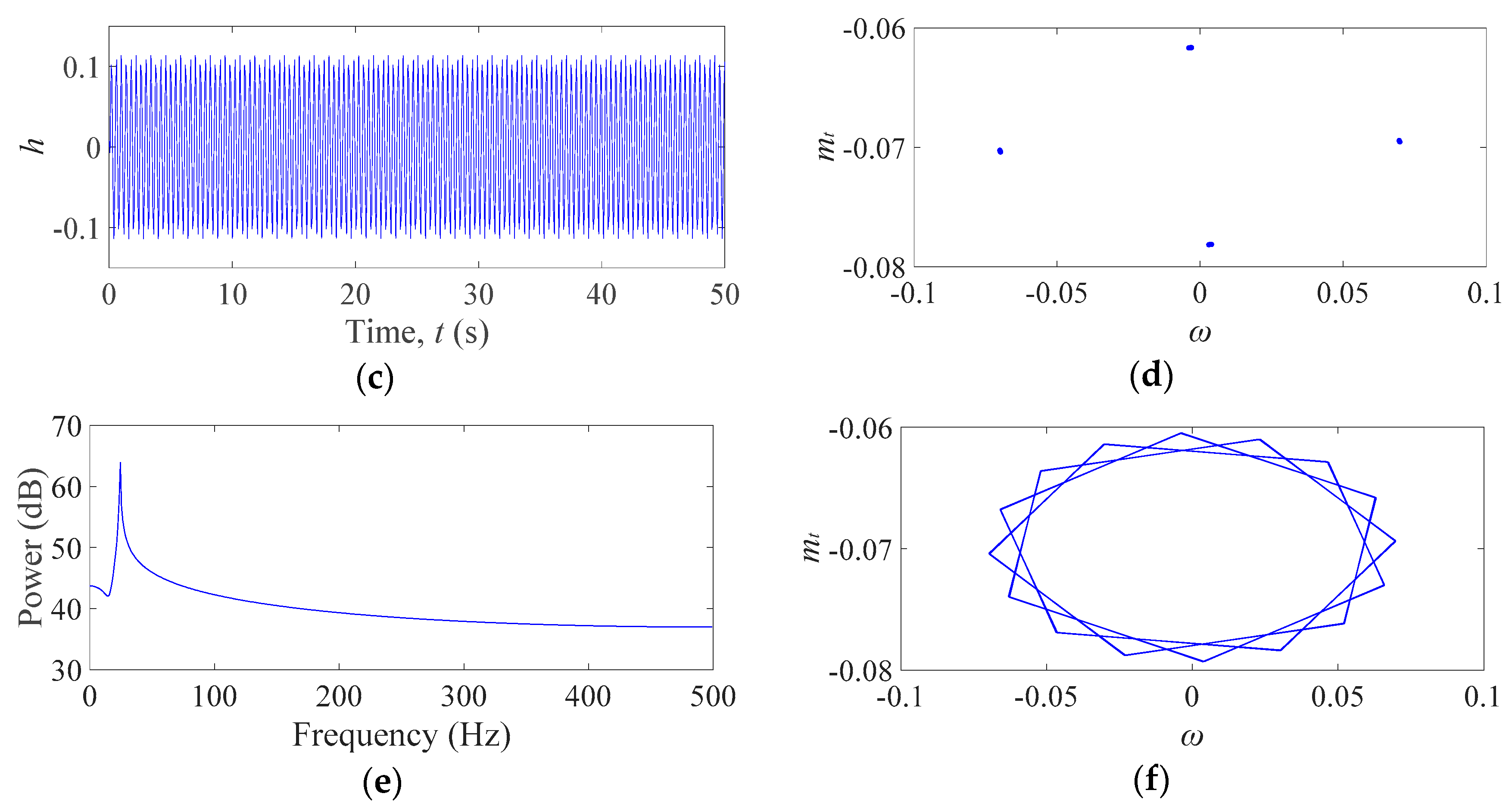
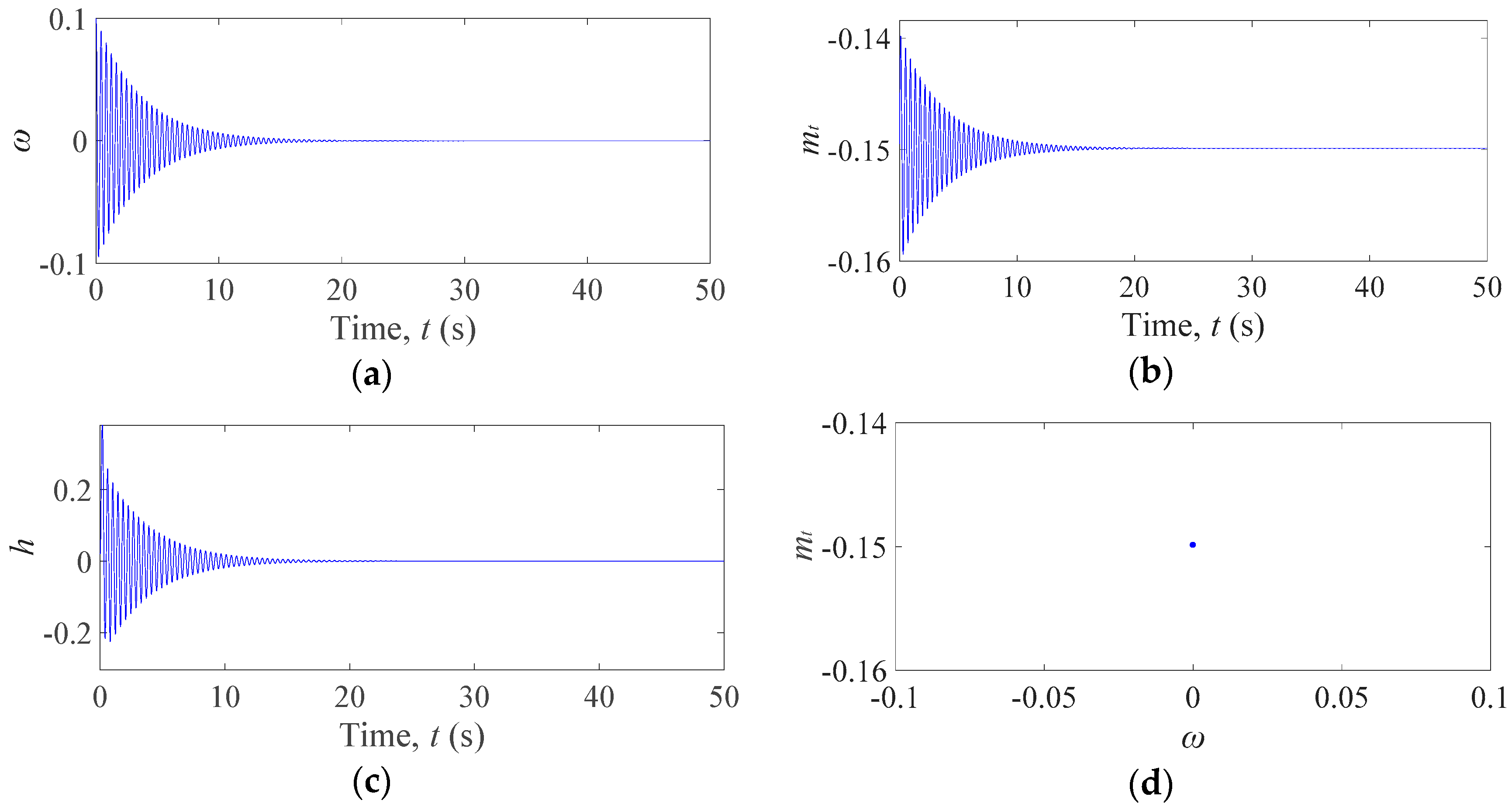
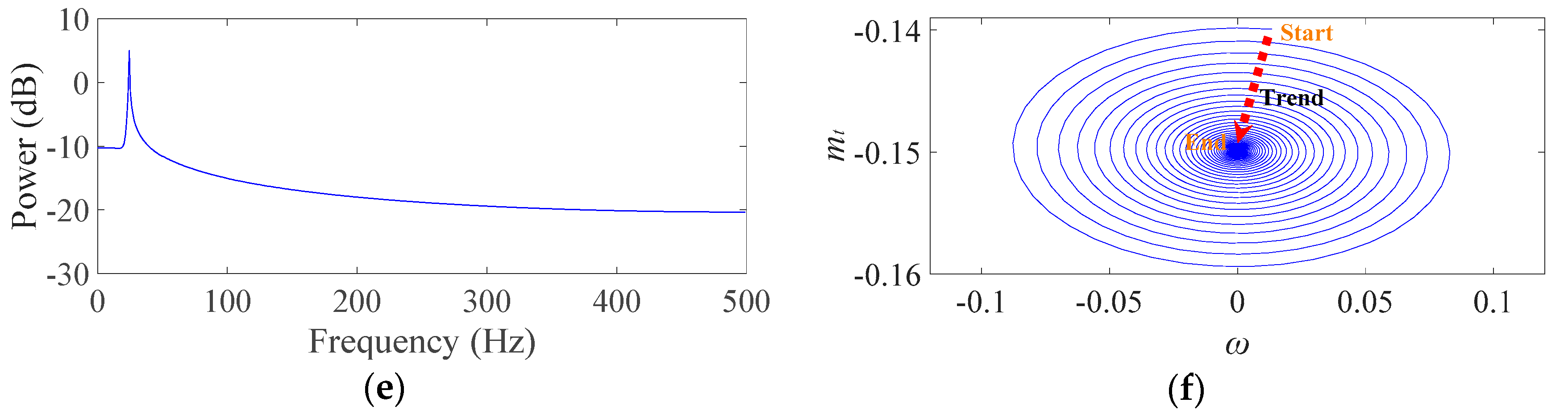
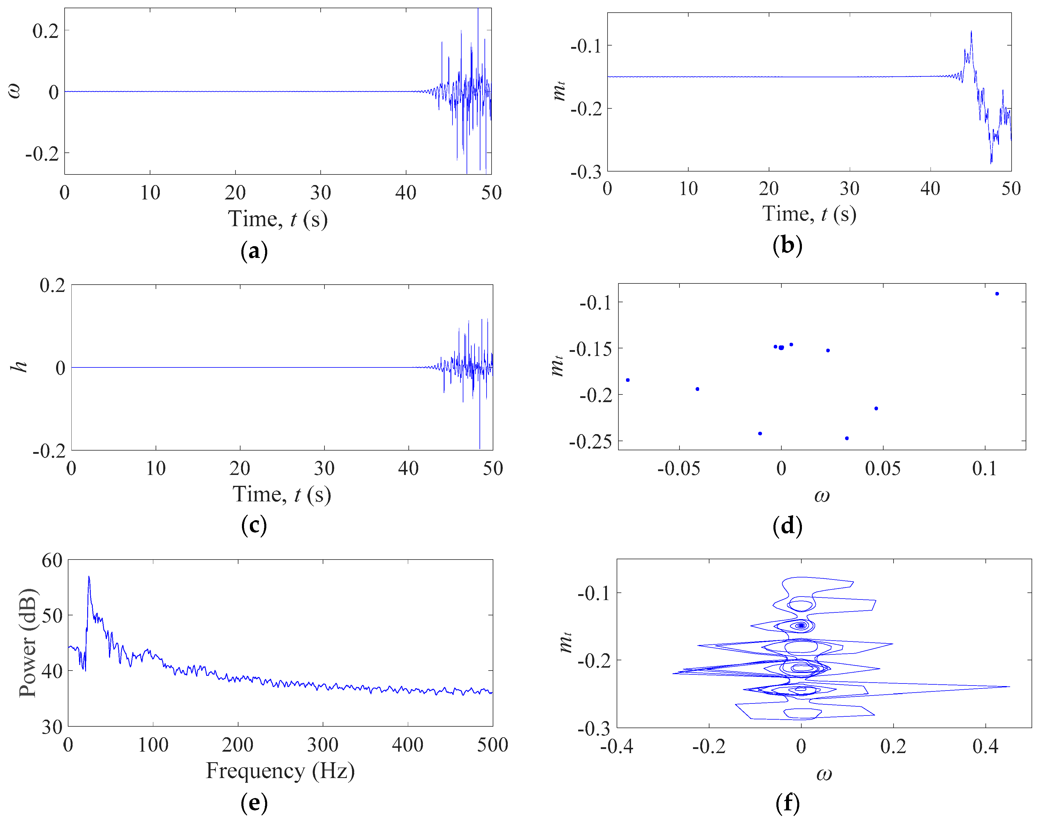
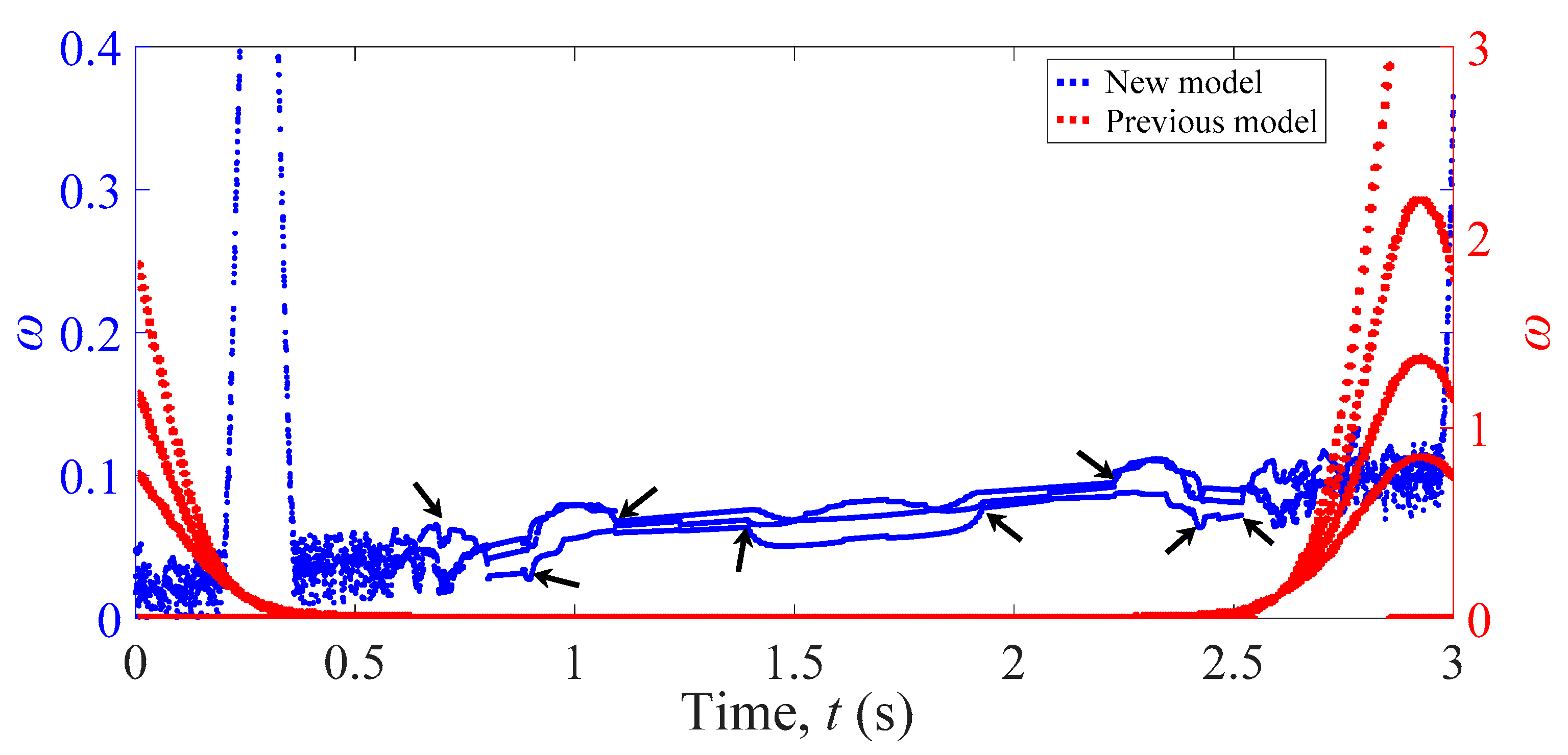
3. Nonlinear Dynamic Analyses of the Hydro–Turbine Governing System

In this section, the nonlinear dynamic methods will be used to investigate the nonlinear dynamic characteristics of the HTGS in the process of the load shedding. Specifically, bifurcation diagrams, time series, Poincare maps, power spectrums and phase planes are applied in the study. Keeping PID parameters at constant values, the Runge–Kutta method is applied in the numerical experiment. The step–size is 0.01, the iteration steps are 5000 for each time of simulation, and the initial values [24,31] specified for the computation are as follows: [$x_1$, $x_2$, $x_3$, $\delta$, $w$, $y$, $h$, $q$, $m_t$] = [0.001, 0.001, 0.001, 0.01, 0.01, 0.01, 0.01, 0.01, 0.01]. In addition, considering the complex nonlinear characters of the HTGS and the elastic water hammer of the penstock in the load shedding transient process, the hydro–turbine structure and the HTGS parameters are selected based on some published papers [24,31,34,35], which are listed as follows: ${\omega }_B$ = 314, D = 0.5, $E_q^{\prime }$ = 1.35, $x_{d\mathrm{\Sigma }}^{\prime }$ = 1, $x_{d\mathrm{\Sigma }}^{\prime }$ = 2, V_s = 1, T_y= 1, T_ab = 8, T_w = 2, k_p = 2, k_i = 1, k_d = 5, D₁ = 1.4 m, b₀ = 0.511 m, Z₀ = 16, W_r = 300$\pi$ rad/min, Q_r = 12.75 m³/s, H_r = 30.5 m, Y_r = 0.24 m, r = 0.7 m, A = 0.49π m².

Bifurcation diagrams of the relative deviation of the rotational speed (ω) and the relative deviation of the mechanical torque (m_t) with time from 0 s to 3 s in the load shedding process are shown in Figure 3a,b, respectively.

As an overview, first, from Figure 3a,b, the whole process can be divided into four parts according to differences of the nonlinear dynamic phenomena, which have been marked in figures. In part 1, the relative deviation of the rotational speed (ω) and the relative deviation of the mechanical torque (m_t) maintain a chaos–1 state at 0 s < t < 0.202 s. In part 2, a huge jump appears at t = 0.202 s whether the relative deviation of the rotational speed (ω) or the relative deviation of the mechanical torque (m_t). Then they turn back to the previous state at t = 0.362 s. In part 3, the two system parameters transit from chaos to periodic oscillation when 0.362 s < t < 2.518 s. In part 4, the relative deviation of the rotational speed (ω) and the relative deviation of the mechanical torque (m_t) change from the periodic oscillation, to the quasi–period oscillation, to the chaos.

Second, there are two typical fluctuations in bifurcation diagrams of the relative deviation of the rotational speed (ω) and the relative deviation of the mechanical torque (m_t) at t = 0.202 s and t = 2.976 s, respectively.

The first fluctuation appears at the start of the guide vane closure process. This phenomenon means that the hydro–turbine generator unit operates at an extremely unstable state in this condition. In actual engineering, a huge variation will also arise in this condition for the hydro–turbine generator unit. Concretely, when the guide vane closes quickly, the pressure of the penstock and the rotational speed will increase sharply, and the hydraulic imbalance and the mechanical vibration will also be aggravated. All these phenomena indicate that the hydro–turbine generator unit maintains an extremely precarious state, which is consistent with the analysis results of the bifurcation diagrams shown in Figure 3. Therefore, it is necessary to pay more attention to the sudden close of the guide vane in the operation.

The second fluctuation appears at the end of the guide vane closure process, which also suggests that the hydro–turbine generator unit is unstable. In actual engineering, in this condition, the rotational speed is greater than the previous, and the inertia of the water cannot be effectively counteracted in the guide vane closure process, so the water pressure in the penstock increases with the changing of the time. In the end of the guide vane closure process, the water hammer and mechanical dynamic unbalance have significant impacts on the hydro–turbine generator unit, which can lead to the instability of hydro–turbine generator unit. According to above analyses, the influences of the elastic water hammer and the mechanical dynamic unbalance are still remarkable in the load shedding process, especially, in the end of the load shedding process, which should also be paid attention to in the operation.

For further studying dynamic characteristics of the HTGS, as is shown in Figure 4, Figure 5, Figure 6, Figure 7 and Figure 8, time series, Poincare maps, power spectrums and phase planes at some representative points are presented.

For t = 0.1 s, as is shown in Figure 4, time waveforms of the rotational speed (ω), the mechanical torque (m_t), and the hydro–turbine head (h) tend to divergence with the increasing time. And there are a lot of chaotic points in Poincare map. Then in power spectrum, there are two peaks at frequency = 20.51 Hz and frequency = 24.41 Hz, respectively, and there is a faint peak at frequency = 56.64 Hz. Besides, the phase plane shows that the phase locus (m_t–ω) tents to infinity. Based on above analyses, all these results indicate that the HTGS tend to an unstable state at t = 0.1 s.

Figure 5 shows the time series, Poincare map, the power spectrum and phase plane at t = 0.645 s. Concretely, the rotational speed (ω), the mechanical torque (m_t), and the hydro–turbine head (h) always maintain a quasi–periodicity motion. The Poincare map is a circle comprised by many discrete points. And there is only one peak in power spectrum at frequency = 24.41 Hz. The phase locus (m_t–ω) is an annulus limited to a limit–cycle. In this condition, the HTGS maintains a critical state. The whole HTGS can work normally, but, when a small disturbance appears, this balance could be broken easily. Therefore, it is an omen for the instability of the HTGS.

Dynamic behaviors of the HTGS at t = 1.257 s are shown in Figure 6. Obviously, the rotational speed (ω), the mechanical torque (m_t) and the hydro–turbine head (h) always keep a period–3 motion. Interestingly, it can be found that in Figure 3b, one period is hidden in the bifurcation diagram of the mechanical torque (m_t), but it cannot influence the results of the stability analyses. Then the Poincare map shows four discrete points. Besides, the power spectrum in this condition is similar with the chart at t = 0.645 s. Finally, it can be found that the phase locus (m_t–ω) is also limited to a limit–cycle. Hence, according to these analyses for Figure 6, it is obvious that the operation state of the HTGS at t = 1.257 s is similar with t = 0.645 s, and both of them keep a critical stable state. Differing from Figure 5, the system state at t = 1.257 s is a kind of critical stable state with period–3 motion.

Responses of the HTGS at t = 2.534 s are illustrated in details in Figure 7. Time waveforms of the rotational speed (ω), the mechanical torque (m_t) and the hydro–turbine head (h) converge to stable values, respectively. In addition, there is only one point in Poincare map. And the power spectrum is also similar with the chart at t = 0.645 s shown in Figure 5d. More obviously, from Figure 7f, it can be gotten that the phase locus (m_t–ω) is converging to a steady value with time. According to analyses for Figure 7, the HTGS is stable in this condition. And the HTGS can work effectively to maintain the safety and stability of the hydropower station.

Finally, Figure 8 shows responses of the HTGS at t = 2.972 s. Time waveforms of the rotational speed (ω), the mechanical torque (m_t) and the hydro–turbine head (h) all gradually increase with the time. Nevertheless, they are different from time series at t = 0.1 s. Specifically, the main difference of them is that time waveforms at t = 2.972 s tend to chaos, while time waveforms at t = 0.1 s are regular. The Poincare map is also composed by many chaotic points. In addition, differing from previous four power spectrums, a lot of small peaks appear at t = 2.972 s. Interestingly, the phase plane contains six vortexes, which is a typical character of chaos.

According to these analyses, the HTGS is unstable in this condition. Combining the analysis results of the bifurcation diagrams, it can be inferred that the instability of the HTGS in this condition mainly results from the water hammer. Therefore, close attention should be paid to the water hammer of the penstock whether in the scientific research or in the actual operation in engineering.

In this research, a novel nonlinear mathematical model of the HTGS has been presented, and comparing with a typical model in previous papers, it is more reasonable in describing nonlinear dynamic characteristics of the HTGS. Concretely, the comparison of the bifurcation diagram between the novel nonlinear mathematical model and the previous model is shown in Figure 9.

First, the previous typical comparison model is introduced from [24], in which the six hydro–turbine transfer coefficients (e_my, e_mh, e_mω, e_qy, e_qh and e_qω) in major fluctuation are calculated using an approximation method. Second, the system parameters are kept consistent with the previous model.

From Figure 9, in the new model, when 0.7 s < t < 2.4 s, the rotational speed maintains a transition stage including the instability state, critical stable state and stable state. The relative deviation of the rotational speed (ω) in bifurcation diagram is larger than zero. However, in the previous model, the rotational speed always maintains stable state. The relative deviation of the rotational speed (ω) changes around zero all the time. In fact, in the load shedding transient process, the relative deviation of the rotational speed (ω) in bifurcation diagram should be larger than zero. Because of the water hammer, the mechanical unbalance, and other instability factors, the rotational speed cannot always remain in a stable state in this range. Therefore, the new model is more accurate on describing the state of the HTGS in the load shedding transient process.

Besides, some details need to be paid attention to. From the bifurcation diagram of the new model, it can be found that there are a lot of turning points, which have been marked in Figure 9 by black arrows. However, these turning points are hidden in the previous model. In fact, when the load shedding transient appears in the actual hydropower station, the rotational speed will be influenced by many unstable factors, so the small turning and fluctuation are common in the load shedding process for the hydropower station.

Based on the above analyses, it is apparent that the new model of the hydro–turbine transfer coefficients is more reasonable in the analyzing the nonlinear dynamic characteristics of the HTGS.

Finally, it is also significant to discuss the reasons of the differences between the previous model and the new model. In previous model, the six hydro–turbine transfer coefficients are calculated using an approximation method, which are only the function of the time. However, in the new model, the six hydro–turbine transfer coefficients are the function of the hydro–turbine head (h), the rotational speed (ω), the guide vane opening (y), and the hydro–turbine flow (q). Therefore, the new model of the transfer coefficients can reflect complex relationships of the system parameters more accurately. And it also can describe more details of the nonlinear dynamic characteristic of the HTGS.

4. Conclusions

In this study, considering that the six hydro–turbine transfer coefficients will change with the operation condition of the hydro–turbine generator unit, we propose a novel and creative calculation method of the six hydro–turbine transfer coefficients based on their definitions and the hydro–turbine internal characteristics, in which the transfer coefficients are complex nonlinear functions of the hydro–turbine head, the hydro–turbine flow, the rotational speed, and the guide vane opening. Then, a novel nonlinear mathematical model is established for the HTGS in the load shedding transient process. Finally, the nonlinear dynamic characteristics of the HTGS are discussed from the perspective of nonlinear dynamics and the engineering practice, and the advantages of the novel nonlinear mathematical model are also presented by comparing with the previous model.

According to the numerical simulation results in Section 3, some meaningful conclusions are drawn as follows: first, the HTGS presents a lot of complex nonlinear dynamic behaviors in the load shedding transient process. Second, two drastic unstable states will appear at the start and the end of the guide vane closing process, respectively, which should be paid more attention to for the security and stability of the hydro–turbine generator unit. Third, some small turning points are also found in the middle of the guide vane closing process. Finally, the comparison results indicate that the new hydro–turbine transfer coefficient model is more reasonable than the previous models. More importantly, these results could provide some theoretical references for the operation of the hydropower stations during the load shedding transient process.

References

1. Li, B.; Li, T.; Xu, N.W.; Dai, F.; Chen, W.F.; Tan, Y.S. Stability assessment of the left bank slope of the Baihetan Hydropower Station, Southwest China. Int. J. Rock Mech. Min. Sci. 2018, 104, 34–44. [Google Scholar] [CrossRef]
2. Giosio, D.R.; Henderson, A.D.; Walker, J.M.; Brandner, P.A. Rapid Reserve Generation from a Francis Turbine for System Frequency Control. Energies 2017, 10, 496. [Google Scholar] [CrossRef]
3. Wang, W.Y.; Chen, Q.J.; Liang, X.; Dou, J.Z. A novel multidimensional frequency band energy ratio analysis method for the pressure fluctuation of Francis turbine. Math. Probl. Eng. 2018, 2018, 3494785. [Google Scholar] [CrossRef]
4. Jia, J.S. A technical review of hydro–project development in China. Engineering 2016, 2, 302–312. [Google Scholar] [CrossRef]
5. Trivedi, C.; Cervantes, M.J.; Gandhi, B.K. Investigation of a High Head Francis Turbine at Runaway Operating Conditions. Energies 2016, 9, 149. [Google Scholar] [CrossRef]
6. Ghidaoui, M.S.; Zhao, M.; McInnis, D.A.; Axworthy, D. H. A Review of Water Hammer Theory and Practice. Appl. Mech. Rev. 2005, 58, 49–76. [Google Scholar] [CrossRef]
7. Bergant, A.; Simpson, A.R.; Tijsseling, A. S. Water hammer with column separation: A historical review. J. Fluids Struct. 2006, 22, 135–171. [Google Scholar] [CrossRef]
8. Tijsseling, A.S. Water hammer with fluid–structure interaction in thick–walled pipes. Comput. Struct. 2007, 85, 844–851. [Google Scholar] [CrossRef]
9. Xu, B.B.; Chen, D.Y.; Tolo, S.; Patelli, E.; Jiang, Y.L. Model validation and stochastic stability of a hydro–turbine governing system under hydraulic excitations. Int. J. Electr. Power Energy Syst. 2018, 95, 156–165. [Google Scholar] [CrossRef]
10. Zhang, H.; Chen, D.Y.; Wu, C. Z.; Wang, X.Y. Dynamics analysis of the fast–slow hydro–turbine governing system with different time–scale coupling. Commun. Nonlinear Sci. Numer. Simul. 2018, 54, 136–147. [Google Scholar] [CrossRef]
11. Zhou, W.; Lou, C.Z.; Li, Z.S.; Lu, L.; Yang, H.X. Current status of research on optimum sizing of stand–alone hybrid solar–wind power generation systems. Appl. Energy 2010, 87, 380–389. [Google Scholar] [CrossRef]
12. Castronuovo, E.D.; Lopes, J.A.P. On the optimization of the daily operation of a wind–hydro power plant. IEEE Trans. Power Syst. 2004, 19, 1599–1606. [Google Scholar] [CrossRef]
13. Fang, W.; Huang, Q.; Huang, S.Z.; Yang, J.; Meng, E.H.; Li, Y.Y. Optimal sizing of utility–scale photovoltaic power generation complementarily operating with hydropower: A case study of the world’s largest hydro–photovoltaic plant. Energy Conv. Manag. 2017, 136, 161–172. [Google Scholar] [CrossRef]
14. Kougias, I.; Szabó, S.; Monforti–Ferrario, F.; Huld, T.; Bódis, K. A methodology for optimization of the complementarity between small–hydropower plants and solar PV systems. Renew. Energy 2016, 87, 1023–1030. [Google Scholar] [CrossRef]
15. Chang, J.; Xiao, Z.; Wang, S. Neural network model predict control for the hydroturbine generator set. In Proceedings of the 2003 International Conference on Machine Learning and Cybernetics, Xi’an, China, 5 November 2003; Volume 2–5, pp. 540–543. [Google Scholar] [CrossRef]
16. Eker, I. Governors for hydro–turbine speed control in power generation: A SIMO robust design approach. Energy Conv. Manag. 2003, 45, 2207–2221. [Google Scholar] [CrossRef]
17. Khodabakhshian, A.; Hooshmand, R. A new PID controller design for automatic generation control of hydro power systems. Int. J. Electr. Power Energy Syst. 2010, 32, 375–382. [Google Scholar] [CrossRef]
18. Ren, M.F.; Wu, D.; Zhang, J.H.; Jiang, M. Minimum entropy–based cascade control for governing hydroelectric turbines. Entropy 2014, 16, 3136–3148. [Google Scholar] [CrossRef]
19. Chen, Z.H.; Yuan, X.H.; Ji, B.; Wang, P.T.; Tian, H. Design of a fractional order PID controller for hydraulic turbine regulating system using chaotic non–dominated sorting genetic algorithm II. Energy Conv. Manag. 2014, 84, 390–404. [Google Scholar] [CrossRef]
20. Zhang, R.F.; Chen, D.Y.; Yao, W.; Ba, D.D.; Ma, X.Y. Non–linear fuzzy predictive control of hydroelectric system. IET Gener. Transm. Distrib. 2017, 11, 1966–1975. [Google Scholar] [CrossRef]
21. Chen, D.Y.; Ding, C.; Ma, X.Y.; Yuan, P.; Ba, D.D. Nonlinear dynamical analysis of hydro–turbine governing system with a surge tank. Appl. Math. Model 2013, 37, 7611–7623. [Google Scholar] [CrossRef]
22. Guo, W.C.; Yang, J.D.; Wang, M.J.; Lai, X. Nonlinear modeling and stability analysis of hydro–turbine governing system with sloping ceiling tailrace tunnel under load disturbance. Energy Conv. Manag. 2015, 106, 127–138. [Google Scholar] [CrossRef]
23. Xu, B.B.; Wang, F.F.; Chen, D.Y.; Zhang, H. Hamiltonian modeling of multi–hydro–turbine governing systems with sharing common penstock and dynamic analyses under shock load. Energy Convers. Manag. 2016, 108, 478–487. [Google Scholar] [CrossRef]
24. Zhang, H.; Chen, D.Y.; Xu, B.B.; Wang, F.F. Nonlinear modeling and dynamic analysis of hydro–turbine governing system in the process of load rejection transient. Energy Convers. Manag. 2015, 90, 128–137. [Google Scholar] [CrossRef]
25. Avdyushenko, A.Y.; Cherny, S.G.; Chirkov, D.V.; Skorospelov, V.A.; Turuk, P.A. Numerical simulation of transient processes in hydroturbines. Thermophys. Aeromech. 2013, 20, 577–593. [Google Scholar] [CrossRef]
26. Yang, W.J.; Yang, J.D.; Guo, W.C.; Zeng, W.; Wang, C.; Saarinen, L.; Norrlund, P. A Mathematical Model and Its Application for Hydro Power Units under Different Operating Conditions. Energies 2015, 8, 10260–10275. [Google Scholar] [CrossRef]
27. Terzija, V.V.; Akke, M. Synchronous and asynchronous generators frequency and harmonics behavior after a sudden load rejection. IEEE Trans. Power Syst. 2003, 18, 730–736. [Google Scholar] [CrossRef]
28. Afshar, M.H.; Rohani, M.; Taheri, R. Simulation of transient flow in pipeline systems due to load rejection and load acceptance by hydroelectric power plants. Int. J. Mech. Sci. 2010, 52, 103–115. [Google Scholar] [CrossRef]
29. Yan, D.L.; Wang, W.Y.; Chen, Q.J. Fractional–order modeling and dynamic analyses of a bending–torsional coupling generator rotor shaft system with multiple faults. Chaos Solitons Fractals 2018, 110, 1–15. [Google Scholar] [CrossRef]
30. Xu, B.B.; Chen, D.Y.; Zhang, H.; Zhou, R. Dynamic analysis and modeling of a novel fractional–order hydro–turbine–generator unit. Nonlinear Dyn. 2015, 81, 1263–1274. [Google Scholar] [CrossRef]
31. Lin, D.J. Bifurcation and Chaos of Hydraulic Turbine Governor; Hohai University: Nan Jing, China, 2007. (In Chinese) [Google Scholar]
32. Fang, H.Q.; Chen, L.; Dlakavu, N.; Shen, Z.Y. Basic modeling and simulation tool for analysis of hydraulic transients in hydroelectric power plants. IEEE Trans. Energy. Convers. 2008, 23, 834–841. [Google Scholar] [CrossRef]
33. Shou, M.H.; Zhang, X.B. Study on the dynamic model of the hydro–turbine linear control system. J. Electr. Eng. 1984, 4, 48–57. (In Chinese) [Google Scholar]
34. Xu, B.B.; Yan, D.L.; Chen, D.Y.; Gao, X.; Wu, C.Z. Sensitivity analysis of a Pelton hydropower station based on a novel approach of turbine torque. Energy Convers. Manag. 2017, 148, 785–800. [Google Scholar] [CrossRef]
35. Nagode, K.; Škrjanc, I. Modelling and Internal Fuzzy Model Power Control of a Francis Water Turbine. Energies 2014, 7, 874–889. [Google Scholar] [CrossRef]
Figure 1. The structure diagram of the Francis hydro–turbine governing system.
Energies 11 01244 g001
Figure 2. The closing rule of the guide vane in the load shedding transient process.
Energies 11 01244 g002
Figure 3. Bifurcation diagrams of the HTGS with the time from 0 s to 3 s in the load shedding transient process. (a) The relative deviation of the rotational speed; (b) The relative deviation of the mechanical torque.
Energies 11 01244 g003
Figure 4. Time series, Poincare map, the power spectrum and phase plane with t = 0.1 s. (a) The time series with ωt; (b) The time series with mtt; (c) The time series with ht; (d) Poincare map; (e) The power spectrum; (f) The phase plane with mtω.
Energies 11 01244 g004
Figure 5. Time series, Poincare map, the power spectrum and phase plane with t = 0.645 s. (a) The time series with ωt; (b) The time series with mtt; (c) The time series with ht; (d) Poincare map; (e) The power spectrum; (f) The phase plane with mtω.
Energies 11 01244 g005
Figure 6. Time series plots, Poincare map, the power spectrum and phase plane with t = 1.257 s. (a) The time series with ωt; (b) The time series with mtt; (c) The time series with ht; (d) Poincare map; (e) The power spectrum; (f) The phase plane with mtω.
Energies 11 01244 g006aEnergies 11 01244 g006b
Figure 7. Time series, Poincare map, the power spectrum and phase plane with t = 2.534 s. (a) The time series with ωt; (b) The time series with mtt; (c) The time series with ht; (d) Poincare map; (e) The power spectrum; (f) The phase plane with mtω.
Energies 11 01244 g007aEnergies 11 01244 g007b
Figure 8. Time series, Poincare map, the power spectrum and phase plane with t = 2.972 s. (a) The time series with ωt; (b) The time series with mtt; (c) The time series with ht; (d) Poincare map; (e) The power spectrum; (f) The phase plane with mtω.
Energies 11 01244 g008
Figure 9. The comparison diagram between the novel nonlinear mathematical model and the previous nonlinear mathematical model.
Energies 11 01244 g009