Abstract
In order to elucidate the effect of wall temperature on a diffusion flame–wall interaction, an acetylene diffusion flame in a head-on quenching type was investigated. Direct photography, two-color thermometry, soot-LII (laser-induced incandescence), OH-LIF (laser-induced fluorescence) and numerical simulation with detailed reaction mechanisms were employed to find out the influence mechanism of wall temperature on near-wall combustion performance and emission characteristics. It is clearly shown through optical diagnostics and computation fluid dynamics (CFD) simulation that, compared with cold wall, the high temperature zone for hot wall becomes wider, and the smaller quenching layer is formed due to the higher wall heat flux. High-concentration soot emission is formed primarily near the outer flame far from the wall. CH2O, CO and HC emissions are decreased as wall temperature rises, while the formation of soot and A4 is increased. A diffusion flame–wall interaction structure is proposed to reveal the influence mechanism of wall temperature.
1. Introduction
In some spatially confined combustion environments, such as an engine combustion chamber [1,2,3,4], flame–wall interaction (FWI) will occur. A flame stops propagating towards a cool wall and the flame front is thus quenched, because heat losses are too large to keep chemical reactions near the wall surface. Due to FWI in an engine, the pollutant emissions, such as hydrocarbons (HC) in crevices [5] and carbon monoxide (CO) [6], can be formed, and flame flashback might happen [7,8]. In recent years, the development of engines is in the direction of miniaturization, which increases the surface-to-volume ratio and the FWI will more easily occur, compared to that of larger single-cylinder displacement [9,10]. As a result, FWI becomes a key factor of engine combustion system design and optimization.
FWI causes flame quenching, as described in the previous section. According to the relative position relation between flame propagation direction and wall surface, wall quenching can be divided into two types: head-on quenching (HOQ), where flame propagation is perpendicular to the wall, and side-wall quenching (SWQ), where the flame burns parallel to the wall [11]. Boust et al. [12] ignited a quiescent methane–air mixture by spark electrodes in a constant-volume vessel. Quenching distance was measured through direct visualization and wall heat flux was processed from the time evolution of wall surface temperature, for both head-on and side-wall interactions. To gain a detailed understanding of transport phenomena and reaction in near-wall boundary layers of combustion chambers, Fuyuto et al. [5] measured temperature and species in a quenching boundary layer for a premixed methane–air flat flame side-wall interaction using the two-photon laser-induced fluorescence (LIF) method and revealed the potential and limitation of laser diagnostics techniques for FWI research. Mann et al. [10] determined instantaneous gas phase temperatures using nanosecond coherent anti-Stokes Raman spectroscopy of nitrogen (CARS) in atmospheric methane/air jet flames impinging vertically against a water-cooled stainless-steel wall. They also measured CO concentrations and surface temperatures using two-photon LIF and phosphor thermometry (TP), correspondingly. Dabireau et al. [13] carried out numerical simulation of head-on interactions of premixed and diffusion flames of H2 + O2, and contrasted fluxes of both cases to the wall. Wang et al. [14] studied the questions of turbulent fuel–air–temperature mixing, flame extinction, and wall-surface heat transfer using direct numerical simulation (DNS) for an ethylene–air diffusion flame–wall interaction. They proposed a modified flame extinction criterion that combines the concepts of mixture fraction and excess enthalpy. Desoutter et al. [15] presented a numerical study of the interaction of a premixed flame with a cold wall covered with a film of liquid fuel using DNS. Simulation results showed that the flame–wall distance remained larger with liquid fuel than that of a dry wall, and maximum heat fluxes were smaller.
As mentioned above, advanced optical diagnostics techniques have become an indispensable research method in studying FWI due to their superiorities in high spatial and temporal resolutions and non- or minimally invasive accurate and precise measurement in harsh high-temperature environments. Latterly, for FWI, researchers measure quenching distance, wall heat flux, flame species, temperature and so on using optical diagnostics. It is seen that most previous optical investigations of FWI pay more attention to premixed combustion. However, the study of diffusion flame is apparently rare. Soot, which is significant in the combustion process in a diesel engine, will be easily produced in diffusion flame. So, it is necessary to investigate the FWI in a diffusion flame using optical diagnostics.
Numerical simulation, especially DNS due to the small-scale quenching region, has also played an increasingly important role in the investigation of flame quenching. Considering massive computational costs, only a single-step reaction is usually used in DNS, which could be sufficient for some research targets, but not applicable for pollutant formation mechanisms or evolution of the key intermediate species and radicals in the FWI process. For instant, soot formation, CH2O and OH distributions must be interpreted based on detailed chemical kinetic mechanism. In the past decade, computation fluid dynamics (CFD) coupled with detailed chemical kinetic mechanism has gained importance in the design and improvement of combustion systems [9]. CFD simulation with a suitable small mesh size is also fully capable of satisfying the calculation precision of the thermochemical state near the wall, compared with DNS. Besides, the characteristics of FWI at some extreme wall temperatures, which is hard to implement in optical experiments, can be estimated using CFD in this work. Heinrich et al. [16] simulated the stoichiometric methane/air laminar flame interacting with a cold wall in a side-wall quenching (SWQ) pattern. The simulation used a tabulated chemistry approach (flamelet-generated manifold, FGM) in 2D and 3D, respectively. The results showed that both 2D and 3D FGM simulations could predict the flame structure and major characteristics correctly, such as the temperature, the flame–wall interaction parameter and the reduced quenching distance. However, it had limitations in predicting CO mass fraction distribution near the wall.
In this work, an optical diagnostic system was established for acetylene diffusion flame–wall interaction. Temperature and species (OH and soot) measurements were focused on the near-wall region of stationary laminar impinging flame by means of two-color thermometry, OH-LIF (LIF, laser-induced fluorescence) and soot-LII (LII, laser-induced incandescence). The wall surface temperature (Tw) was controlled by adjustable water-cooling of the wall assembly. Two situations (Tw = 295.5 K and 383 K) were selected for minimum controllable water-cooling temperature and boiled water temperature. CFD simulation coupled with detailed chemical kinetic mechanism was implemented to explore the effects of a wide temperature range (100–700 K). Then, the evolution mechanisms on soot, CO and HC were explained by CFD analysis. The study is significant to understand the flame–wall interaction.
2. Experimental Setup and Approaches
2.1. Acetylene Diffusion Flame–Wall Interaction Device
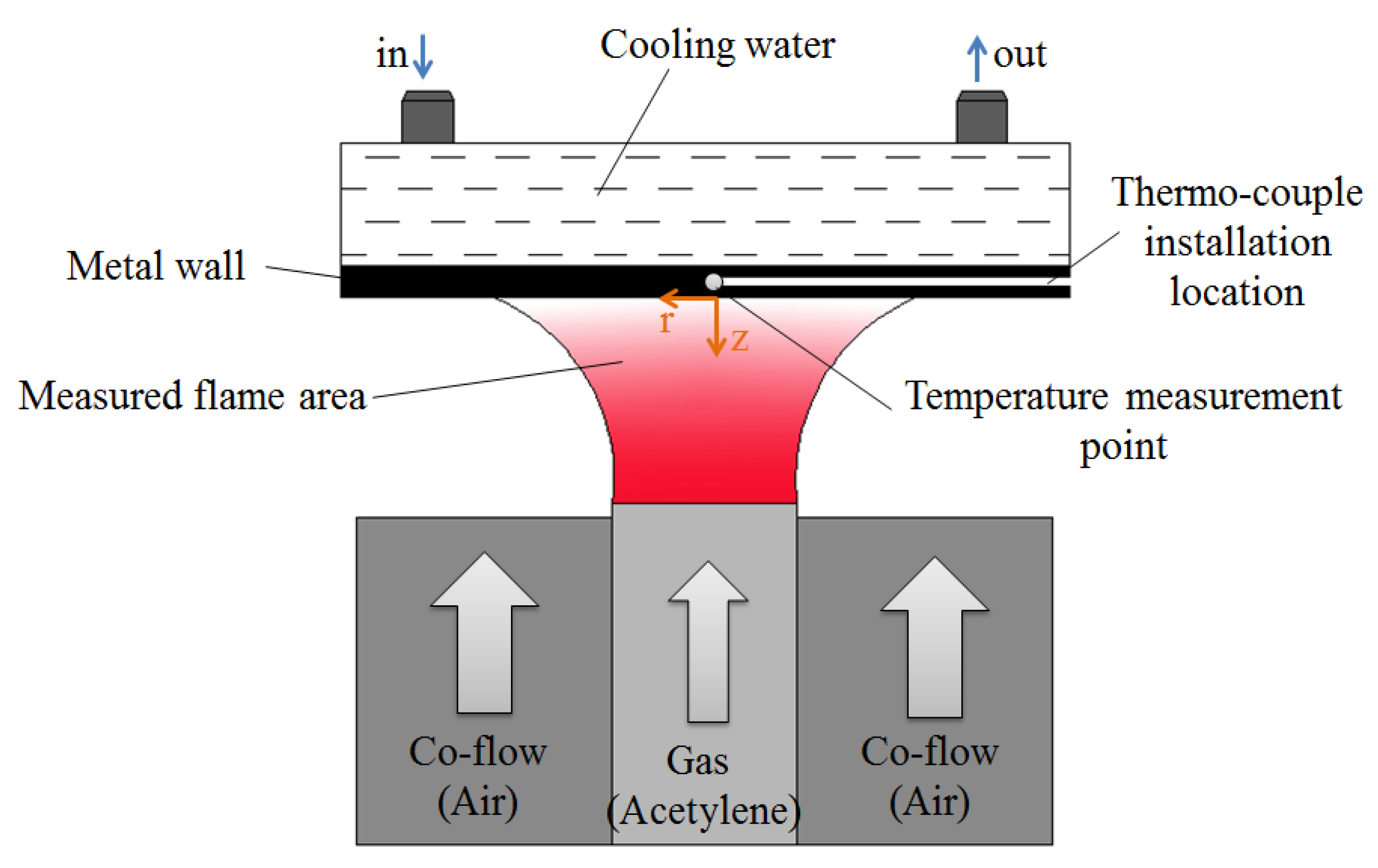
The experiments were conducted based on a McKenna burner, and the configuration of diffusion flame quenching is shown in Figure 1. The burner consists of a hollow fuel nozzle of 8 mm diameter. A cylindrical wall made of stainless steel was fixed at a distance of 7 mm above the fuel nozzle to study the head-on flame–wall interaction. The cylinder exhibited a radius of 50 mm and a thickness of 20 mm. A water cavity was dug for surface cooling in the wall. The surface temperature was controlled using a water-cooling system (YKKY, LX-150, Beijing, China). A K-thermocouple was mounted at 1 mm above the surface to measure the temperature at the central area, and the temperature measuring point lay in the center of the surface. The uncertainty of temperature measurement was ±0.5 K. In order to describe the position relationship of flame in the vicinity of the wall surface, the coordinate system was defined as follows: z-axis was the center axis of the flame, being positive in the upstream direction and zero at the wall surface. R-axis was perpendicular to z-axis and denoted the radical distance, with r = 0 at the centerline of the flame, as shown in Figure 1.
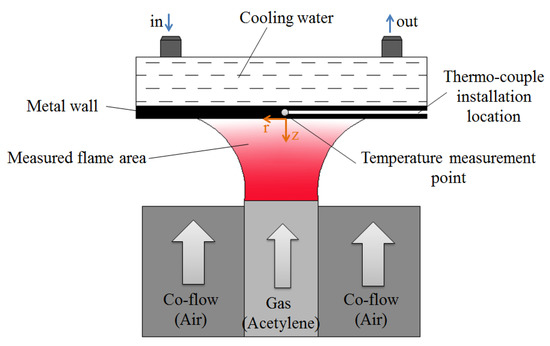
Figure 1.
Schematic diagram of acetylene diffusion flame–wall interaction device.
During acetylene flame–wall interaction, soot was formed in substantial amounts and stuck together on the surface, which would disturb the flame structure in the near-wall region. In the present work, to reduce the soot formation as much as possible and ensure the flame stabilization, acetylene (purity 99.9%) flow rate was controlled at a lower rate of 0.05 L/min using a gas flow meter (ALICT-MC-5slpm). An air (purity 99.9%) co-flow of 30 L/min was used for flame stabilization and confinement. The diameter of the co-flow nozzle was 60 mm; it contained numerous concentric dielectric holes surrounding the fuel nozzle. Table 1 shows the experimental conditions of acetylene diffusion flame–wall interaction. When the cooling water was controlled at the minimum temperature allowed, the wall temperature would be held at 295.5 K (cold wall) with flame heating. Once the water cooling was stopped, the water in the cavity would be heated to a boil, and then the wall temperature would be held at 383 K (hot wall). In this experimental work, two cases in the cold wall and hot wall conditions were investigated. All experiments were carried out at atmospheric pressure.

Table 1.
Experimental conditions of acetylene diffusion flame-wall interaction.
2.2. Optical Setup and Methodology
The optical diagnostics system of flame–wall interaction is displayed in Figure 2. The second harmonics of a Nd: YAG laser (Spectra Physics, Pro-250, Santa Clara, CA, USA) at 532 nm was used to measure the soot formation, and the YAG laser pumped a dye laser (Sirah, CSTR-G-18, Stahnsdorf, Germany) containing a solution of Rhodamine 590 dye, which was pumped by a high-energy pulse at the wavelength of 532 nm. The output pump beam in the wavelength range of 280–284 nm from the dye laser permitted excitation of OH. The laser was introduced to the preset optical path through several laser mirrors, and then a laser light sheet with a height and thickness of approximately 7 mm and 0.8 mm, respectively, was formed by a cylindrical lens group, which was finally directed into the flame region. Optical signals were caught by an intensified CCD (ICCD) camera (Andor, DH720i, Belfast, Northern Ireland) equipped with a UV lens (Nikon, f = 105 mm, f# = 5.6). Since more and more soot adherent to the wall surface grew over time, where normal flame structure could be destroyed, only the first 20 excellent images without damage were captured for analysis under any conditions and the signals were ensemble-averaged to reduce the effect of shot noise.
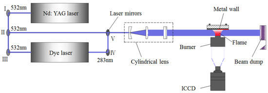
Figure 2.
Schematic diagram of optical diagnostics system for flame–wall interaction.
As in Reference [12], the flame position in the vicinity of the wall was recorded using a direct photography method. It was supposed that the natural luminous zone was associated with the appearance of excited radicals as a result of elementary reactions in the flame. The luminous boundary was the flame front. With the removal of the laser system, the natural luminosity from the flame near the wall was recorded by the ICCD camera. The resulting spatial resolution was 45 × 45 µm2, which could satisfy the resolution requirement of measuring quenching distance.
Due to large soot formations in the acetylene diffusion flame, some temperature measuring methods such as Rayleigh scattering method cannot capture accurate flame temperature distribution. Besides, soot particles have the characteristics of a blackbody, which is in direct proportion to the temperature. So, two-color thermometry based on the continuous soot radiation has been adopted as the primary optical method to measure the near-wall flame temperature in this work. In this technique, not only the laser was required, but also an image doubler (LaVision, VZ14-0591, Göttingen, Germany), which was fixed in the ICCD camera. Two bandpass filters (FWHM = 10 nm) with central wavelengths of 450 nm and 650 nm, respectively, were mounted in the image doubler in front of the collecting lens. Two different colors at 450 nm and 650 nm in the broadband of the soot emission spectrum were synchronously detected by the ICCD camera. The gate width and gain level of the camera were set to 20 μs and 250, respectively. By image cutting, pixel calibration, data extraction and data calculation, the temperature of corresponding pixel in the image could be acquired. The flame temperature T was calculated through Equation (1).
where represents the detection wavelength, is the second Planck’s constant, is the gray body temperature, which has the same intensity as flame temperature at the detection wavelength, the parameter depends on the physical and chemical properties of soot and has a minor effect on flame temperature in visible wavelengths, is set to 1.38 for most fuels.
Laser-induced incandescence (LII) has been widely developed as a qualitative soot diagnostic for application, requiring both high spatial and temporal resolutions in flames [17,18,19,20]. The principle of LII is that soot particles absorb energy from a high-intensity sheet of pulsed laser light within a few nanoseconds, and then the heated particles glow with a blackbody-like incandescence that far exceeds their normal background level. Moreover, according to the blackbody radiation law, within a certain range of detection wavelengths, the radiation from the flame can be ignored before being heated [12]. In this LII technique, the second harmonic (532 nm, 20 mJ/pulse) was used to determine the soot formation and oxidation. The ICCD camera, with a gate width of 20 ns and a gain level of 250, was located perpendicularly to the plane of the laser probe sheet to record the LII signals. The LII signal intensity is proportional to the soot volume fraction. Coupled with the above two-color thermometry system, LII can measure the soot volume fraction in the acetylene diffusion flame near the wall. More detailed introductions on two-color LII can be observed in Reference [17]. The soot volume fraction can be calculated via Equations (2) and (3).
where is the Planck’s constant, is the speed of light, is Boltzmann’s constant, is the detection wavelength (), is the LII signal intensity, is the light sensitivity coefficient of the camera at the wavelength of , which is calibrated by a standard radiation source in the National Institute of Metrology of China [21], is the refractive index of soot, is the wavelength-dependent absorption function of soot, which equals 0.26 in the range of visible light according to References [21,22], and is the actual temperature in the soot region.
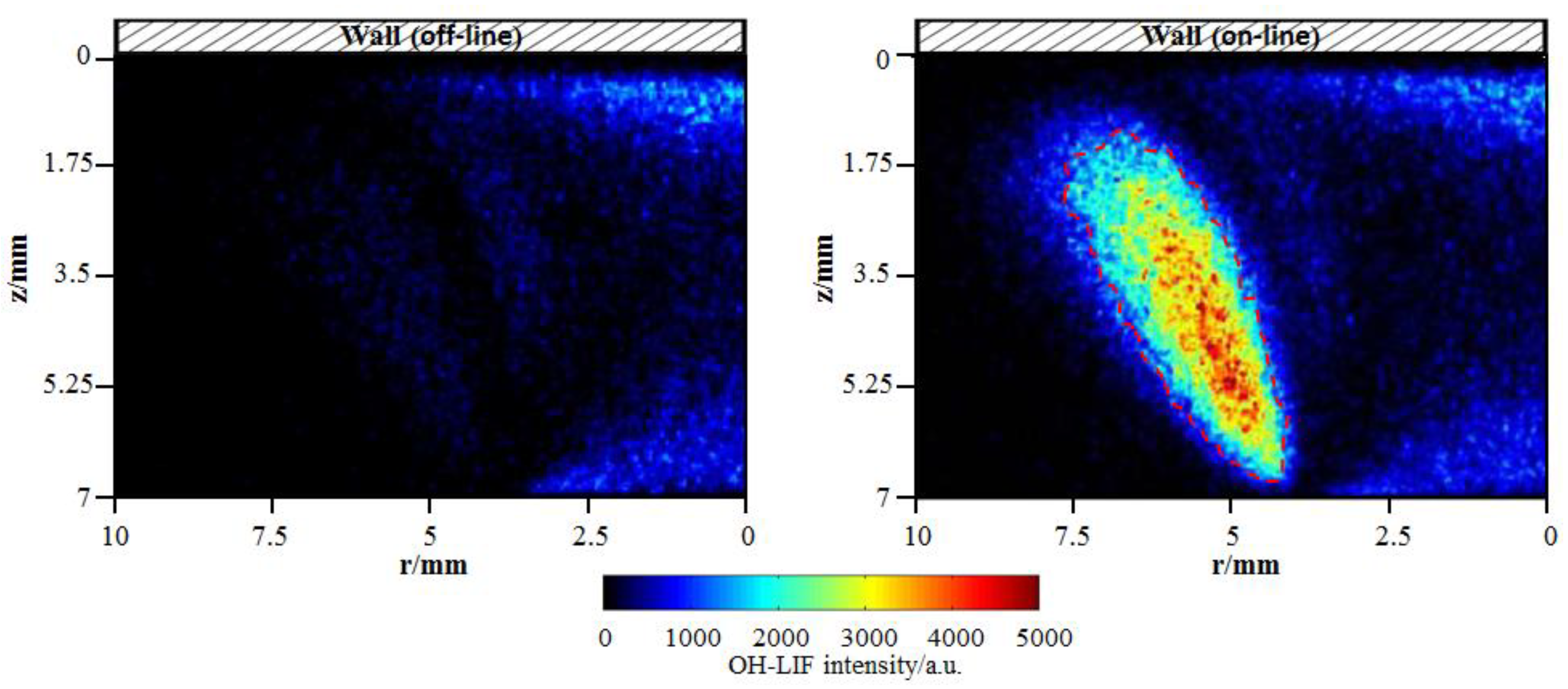
In the present study, the OH measurements were conducted at an excitation of wavelength of 282.91 nm. The gate width and gain level of ICCD was set to 30 ns and 250, respectively. In order to isolate the OH fluorescence signal (at approximately 310 nm) from interference (caused predominantly by laser elastic scattering, polycyclic aromatic hydrocarbon (PAH) fluorescence and soot particle incandescence), a combination of two bandpass filters was placed into the optical path of the camera. The center wavelength of one filter is 315 nm and the total bandwidth is 30 nm. The center wavelength of the other filter is 320 nm and the total bandwidth is 40 nm. Besides, before the formal OH measurement, in order to verify that the measured LIF signals indeed originates from OH and to eliminate the interference, off-line (282.87 nm) OH images, where the laser was tuned off of the OH absorption line, were acquired. Figure 3 presents a comparison between two signals at off-line and on-line wavelengths for cold wall. In the on-line image, the OH fluorescence with significantly high signal-to-noise ratio appears, compared with the quite weak signal intensity in the off-line image. Additionally, for the near-wall diffusion flame, OH should be formed closer to the outer flame, far from the wall where high-temperature heat release happens. The comparison determines that the signal in the marked areas by the red dotted line is indeed solely due to OH radical. Anyhow, some weak signal interference from laser elastic scattering and PAH fluorescence appears.
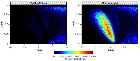
Figure 3.
OH-PLIF (planar laser-induced fluorescence) images at off-line (282.87 nm) and on-line (282.91 nm) wavelengths for cold wall.
3. Numerical Simulation
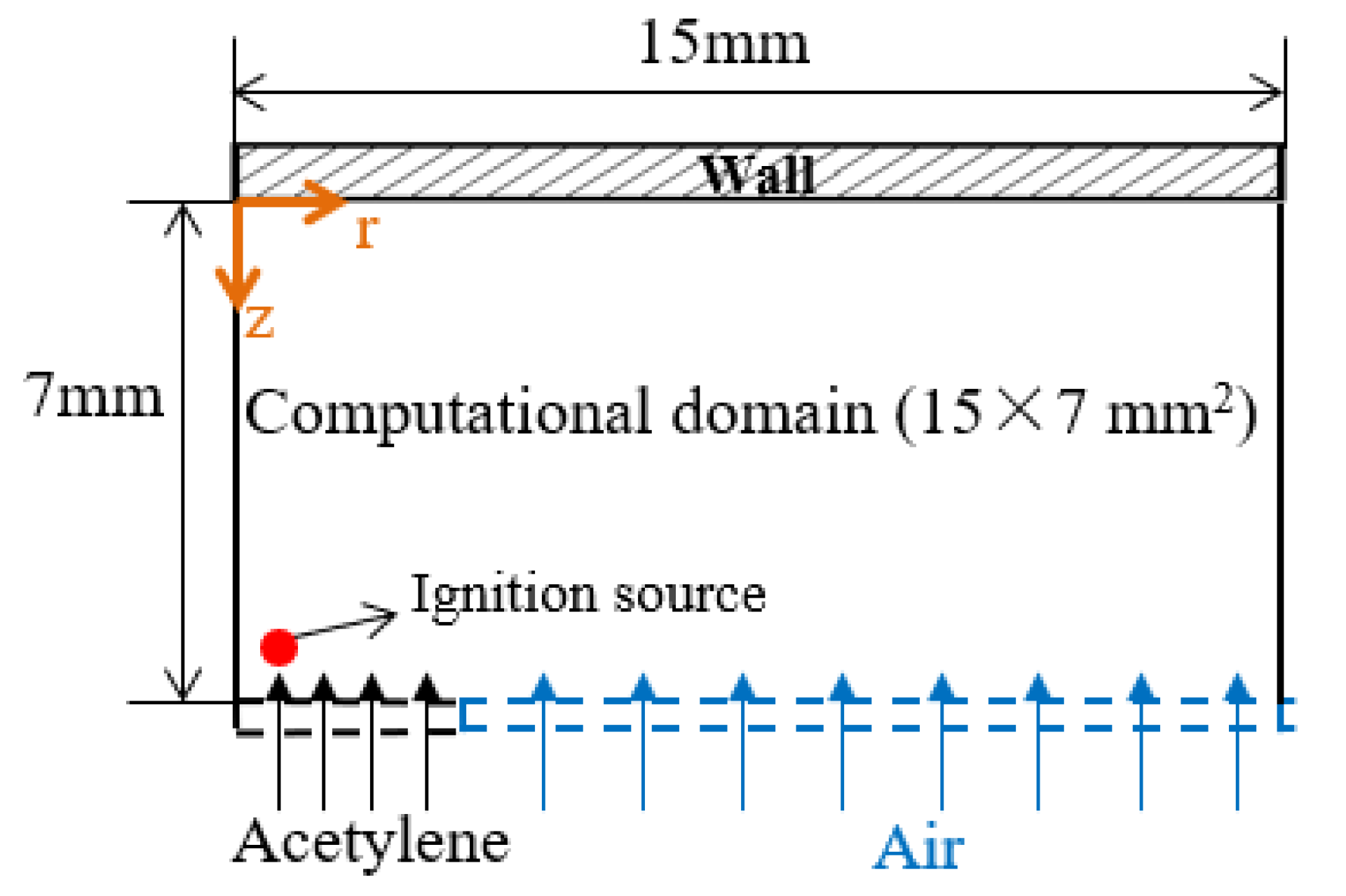
Numerical simulations for acetylene diffusion flame–wall interaction were carried out using a three-dimensional code in Converge. Figure 4 presents the present computational domain setup. Governing equations were mass continuity, Navier–Stokes, species conservation, energy and state equations. The second-order accurate spatial scheme with the finite volume method was adopted. The solver was transient. To reduce the computational costs, a 1/8 sector geometry with the periodic boundaries was used. The computational domain was 15 mm × 7 mm in the flame radius and the wall-normal directions, where the vertical distance between the wall and the burner was consistent with the experiment, and the set domain size in the flame radius direction was bigger to ensure enough space for the full flame development. In addition, the grid was automatically refined using adaptive mesh refinement (AMR) based on temperature. AMR was useful to accurately and precisely simulate the complex flame–wall interaction phenomena. The base cell size was 0.5 mm, and the highest grid resolution was 0.125 mm. The inflow boundary condition, including acetylene flow and air co-flow, was set to the same value as the experimental ones. On the wall, isothermal boundary conditions were imposed. The atmospheric environment was employed at the outlet of the numerical domain. Large eddy simulation (LES) model was implemented in this near-wall flame simulation due to its better predictive capability, and then more flow structures, eddies and vortices were represented on the computational grid. In the present work, a C1–C2 detailed mechanism, including 101 species, 544 reactions [23], was coupled with the CFD models to simulate the diffusion flame–wall interaction process. The elementary reactions involved acetylene formation, oxidation and recombination mechanisms. A source model was used to supply transient ignition energy. The ignition source was located near the central axis of the nozzle outlet and worked in initial period. The result at 1 s after the start time of the simulation, when the flame had been stabilized, was analyzed.
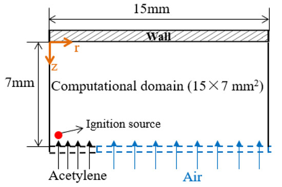
Figure 4.
Computational domain setup.
4. Results and Discussion
4.1. Temperature Distribution and Quenching Distance
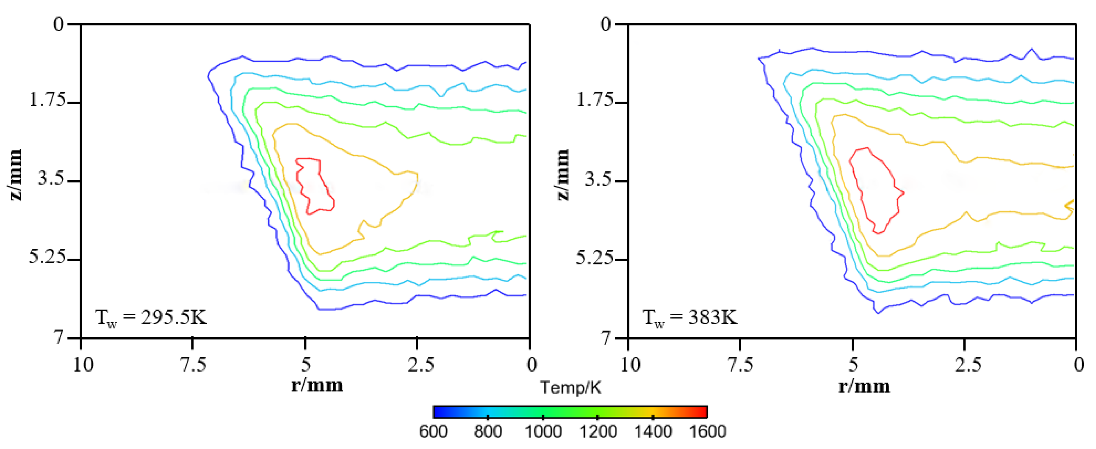
Figure 5 shows the experimental temperature distributions for the 295.5 K and 383 K wall, respectively, and only the left half of flame was analyzed due to the symmetrical flame structure. The temperature was measured using the two-color method, and the measurement error was less than 15 K. The high-temperature zone (>1600 K) is in the outer flame, where adequate oxygen delivery is maintained, and its area becomes wider with increasing Tw, from 295.5 K to 383 K. The measured temperature is very low near the cold wall due to the thermal quenching effect. The low-temperature zone (approximately 600 K) is closer to the wall when Tw increases.
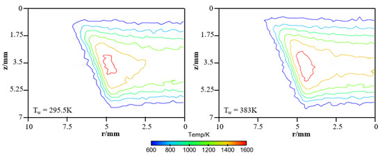
Figure 5.
Experimental temperature distributions for the cold and hot wall.
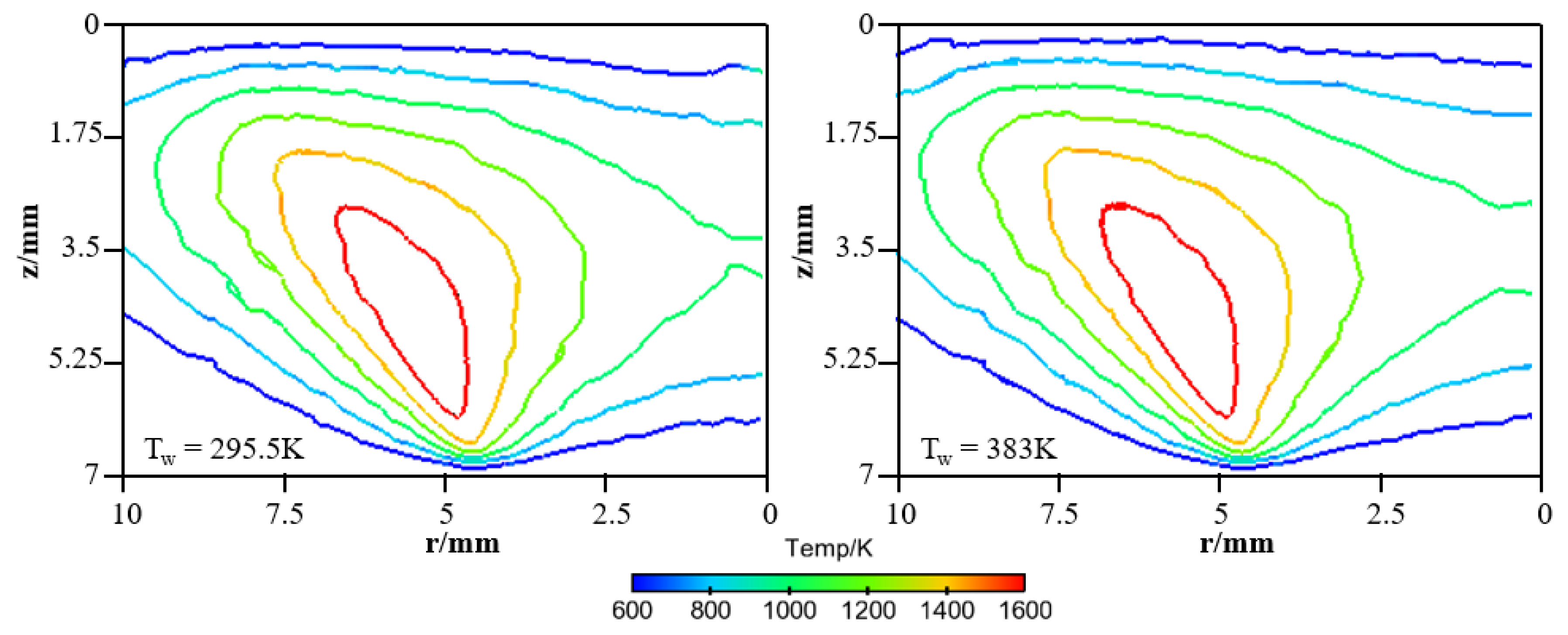
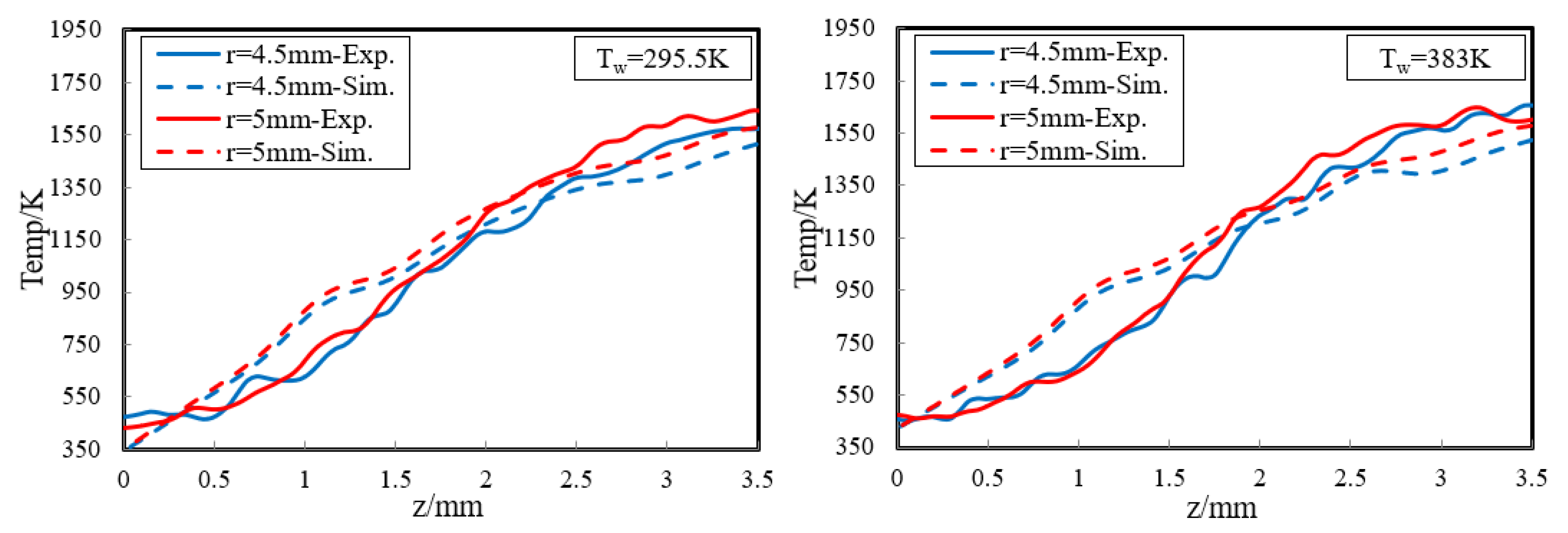
In order to provide a deeper and more intuitive insight of the impact of wall temperature on the diffusion flame–wall interaction, a 3D simulation was implemented. The contours of simulated temperature for the 295.5 K and 383 K wall, respectively, are displayed in Figure 6. The simulated flame structure is similar to the experiment. The low-temperature zone is also closer to the wall as Tw increased. It is also found that there are some differences in temperature distribution between experimental and simulated cases, as seen by comparing Figure 5 and Figure 6. The larger flame zone of simulated cases mainly results from the lower co-flow rate due to the absence of the porous medium, which exists in the experimental burner. The flame is closer to the wall since a catalytic reaction is included in the kinetic mechanism. Previous research also indicated an inert wall could lead to a higher heat release rate and radical concentration at the wall, which contributed to a higher temperature near the wall. However, the objective of the simulation study is to further explore the influence of wall temperature on flame–wall interaction, but not to predict the flame characteristics. Additionally, for more detailed comparison between the two-color data and the simulation results, the wall-normal temperature distributions near the wall (z < 3.5 mm) at r = 4.5 mm and 5 mm for the 295.5 K and 383 K wall are plotted in Figure 7. In a point closer to the wall, there is lower temperature distribution. The comparable results show the present numerical model can represent the effect of wall thermal on temperature distribution near the wall well, as in the optical measurements. So, the numerical model can meet the demand of this work.
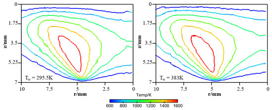
Figure 6.
Simulated temperature distributions for the cold and hot wall.
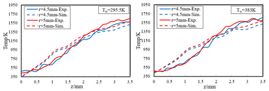
Figure 7.
Wall-normal temperature distributions near the wall (z < 3.5 mm) at r = 4.5 mm and 5 mm for the cold and hot wall.
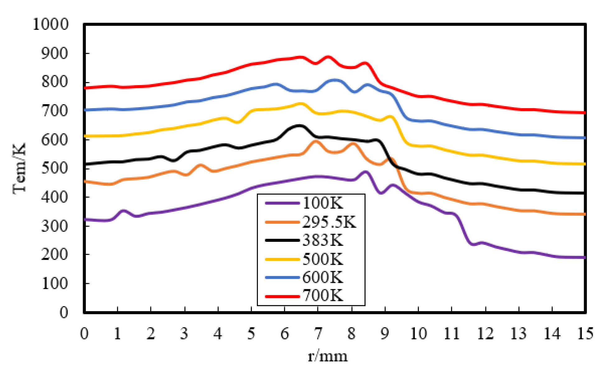
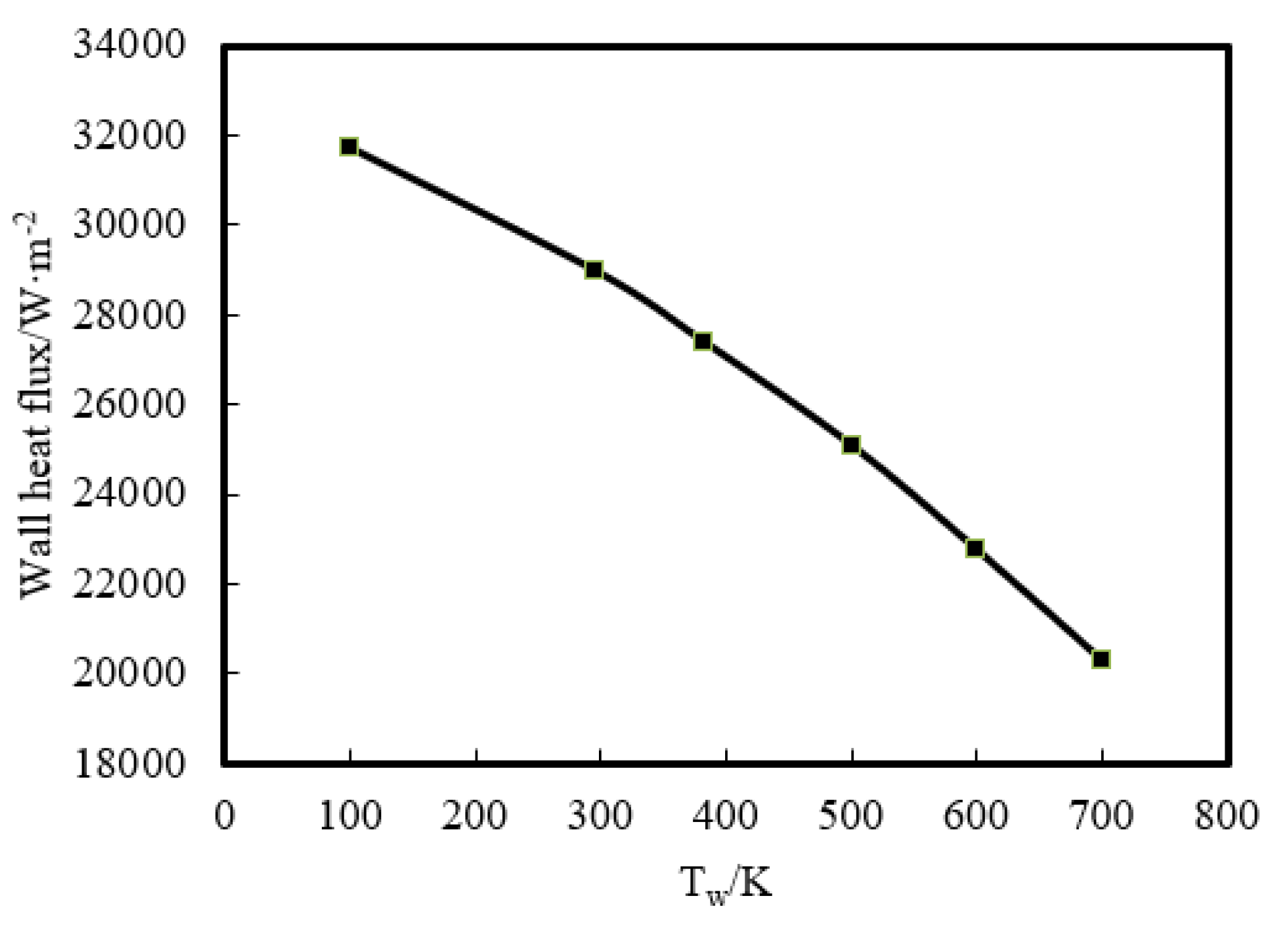
Then, the effect of a wider range of wall temperature, from 100 K to 700 K, on flame–wall interaction was numerically investigated. Figure 8 displays the temperature distribution at z = 0.3 mm. The temperature near the wall goes up with increasing Tw. This indicates that the zone, which is influenced by the high-temperature wall, has a higher temperature due to the stronger heat diffusion from the wall and less wall heat flux. The wall heat flux variation for the range of temperatures used is displayed in Figure 9. The heat flux is found to be the least for the highest wall temperature and the most for the lowest wall temperature, which must lead to a change of quenching distance. It can also be inferred from Figure 8 that the lower Tw contributes to the greater quenching distance.
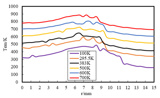
Figure 8.
Temperature distribution at z = 0.3 mm by simulation.
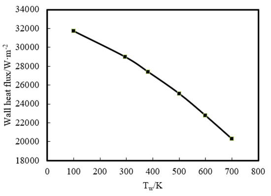
Figure 9.
Wall heat flux variation in 100–700 K wall boundary conditions.
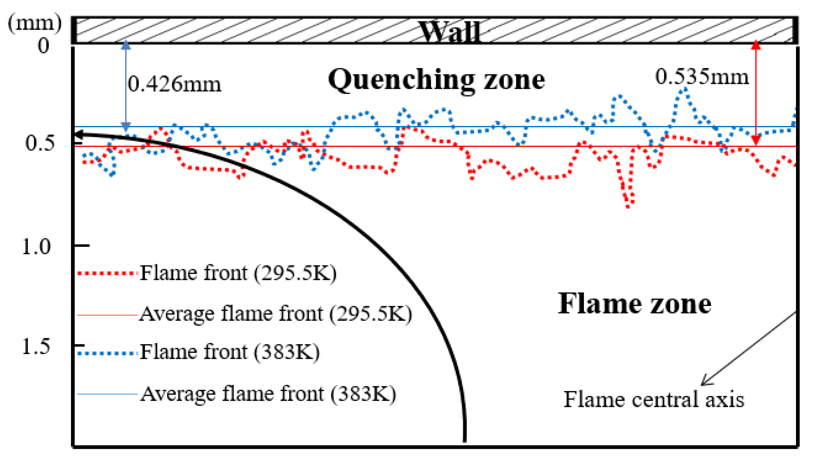
Quenching distance (δq) is one of the most significant parameters directly responsible for unburned hydrocarbon (UHC) emissions and heat loss near the wall. The flame front near the wall can be obtained using direct natural flame luminosity imaging. The quenching distance is defined as the thickness of the dark space between the wall surface and the head of the luminous zone. Figure 10 shows the flame front locations for different experimental wall temperatures (295.5 K and 383 K), and only the left half of flame was analyzed due to the symmetrical flame structure. The flame front was so wrinkled that the average flame front was gained by image preprocessing. During the processing, a quenching distance was measured at the interval of 0.5 mm along the flame radius, and the value of δq was averaged for all the measured points at all wall temperatures. One can see that the head-on quenching distance decreases from 0.535 mm to 0.426 mm as the wall temperature increases from 295.5 K to 383 K. This can be interpreted through the simulated wall heat flux, as presented in Figure 9, and also further verifies the rationality of the simulation model.
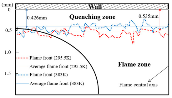
Figure 10.
Flame front locations for different experimental wall temperatures: 295.5 K indicated by red dotted line and 383 K indicated by blue dotted line.
4.2. Emissions Near the Wall
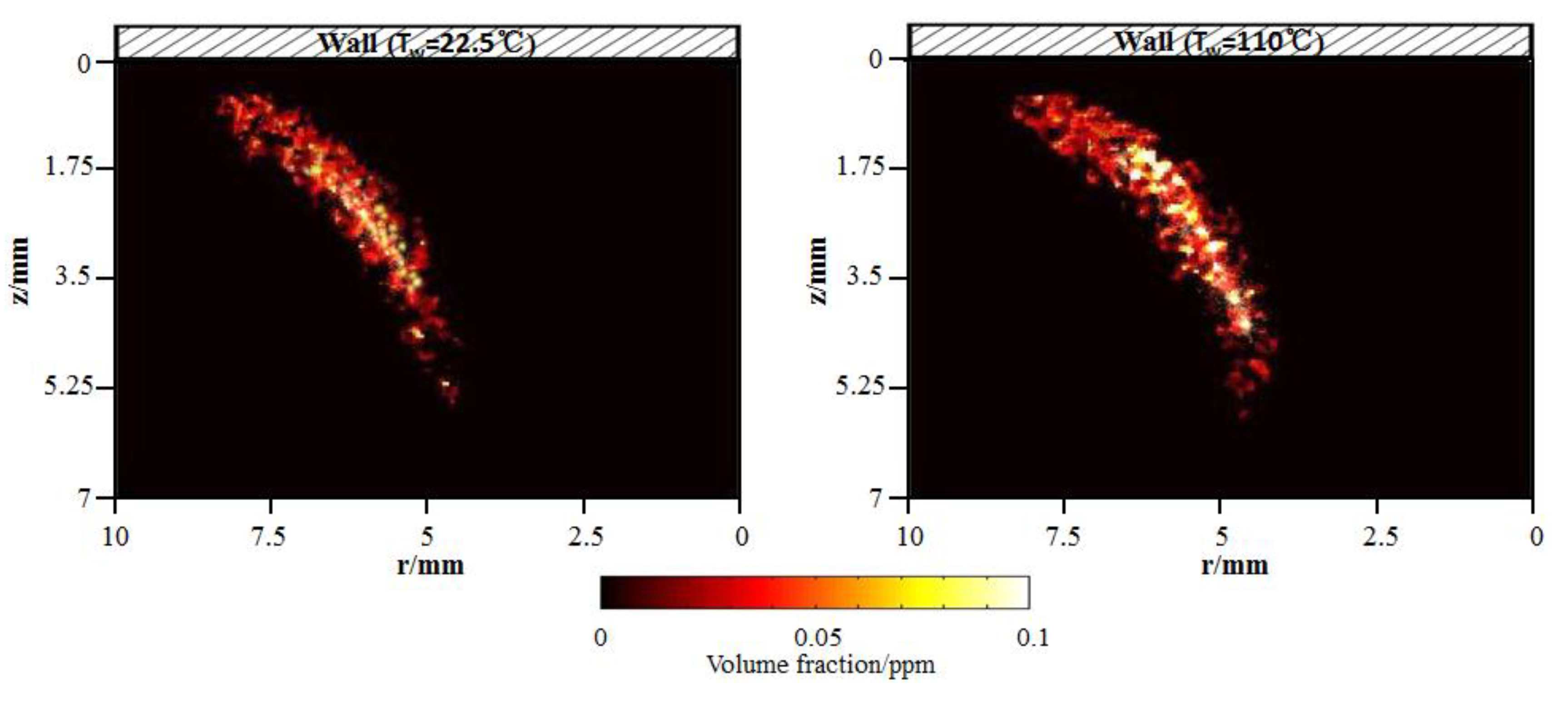
Soot influences the combustion characteristics and emissions in the flame. The effect is dominated by local interactions. For flame–wall interaction, the soot formation and oxidation near the wall is tightly related to the wall thermal. To identify the soot formation mechanism near the wall, LII combined with the two-color method was employed to measure soot quantitatively. Figure 11 shows the flame soot volume fraction distributions for the cold and hot wall. It is apparent that soot is spatially isolated as discontinuous particles. Referring to Figure 4, in both cases, high concentration regions of soot emission appear near the outer flame, far from the wall. The total soot volume fraction increases from 99.08 ppm to 121.68 ppm with the increasing wall temperature from 295.5 K to 383 K. An explanation will be provided in the next paragraph.

Figure 11.
Flame soot volume fraction distributions for cold and hot wall using two-color laser-induced incandescence (LII) by experiments.
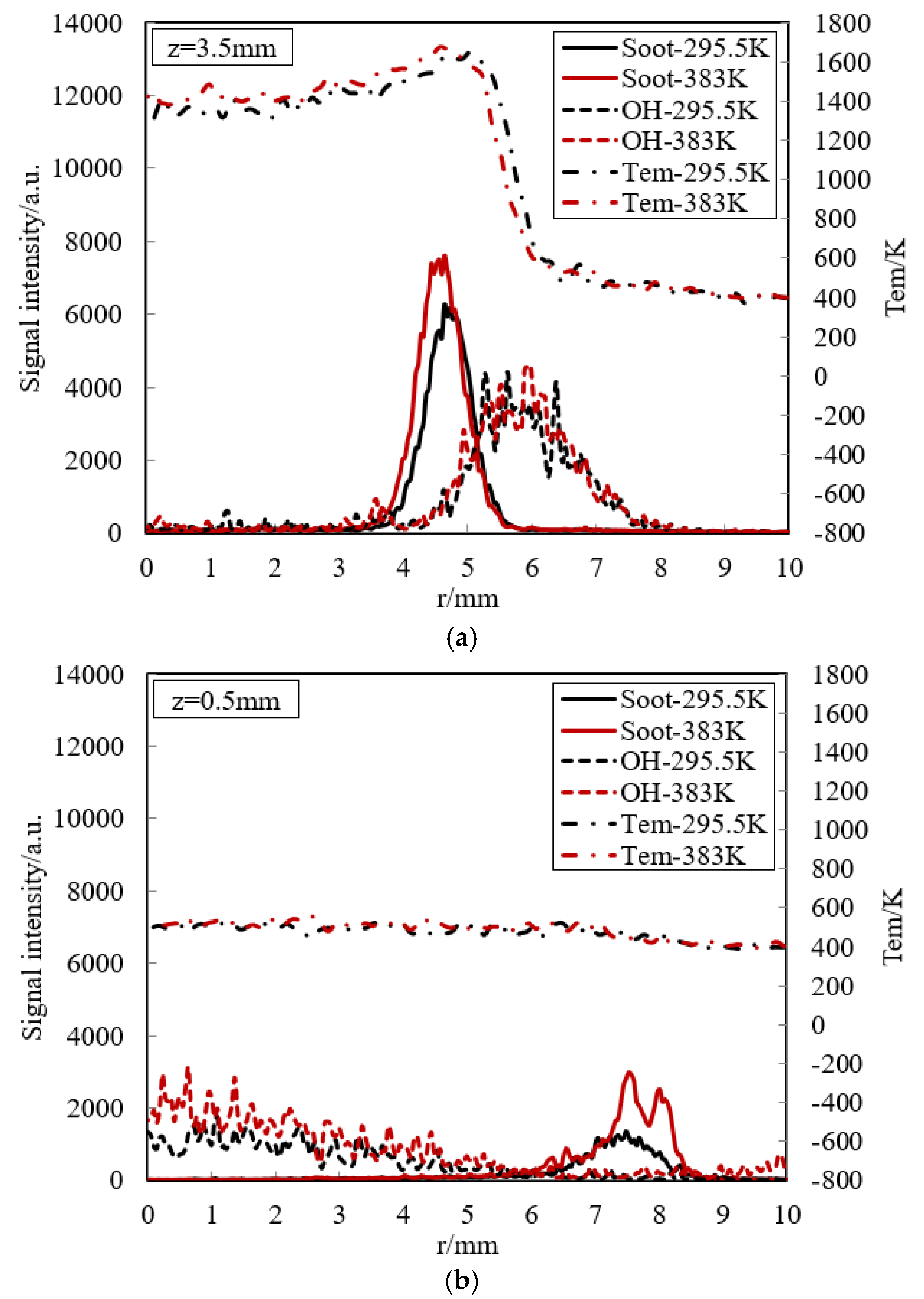
OH is often considered as a useful intermediate species for flame structure research, as well as a good marker of flame front. Figure 12 presents the soot emission, OH radical and temperature at (a) z = 3.5 mm (free flame zone) and (b) z = 0.5 mm (near-wall flame) for the cold and hot walls in the experiment. In the free flame zone, soot is firstly formed along the radius. Soot peak exists in the high-temperature zone, where fuel-rich combustion definitely occurs. This is consistent with soot formation condition. Soot is typically formed in a diffusion flame for hydrocarbon fuels when temperature lies between 1200 K and 1800 K, and its peak appears between 1600 K and 1700 K and the mixture is richer. Soot is consumed where OH formation firstly occurs. The existence of an overlapping region of the soot particles and OH radicals indicates oxidation of the soot. For OH, the location of its peak is just outside the maximum temperature, where it is known to be favorable for OH formation. This peak implies that this location is near the stoichiometric condition. A detailed concentration distribution in the flame will be demonstrated to make a further analysis in the following simulation. Due to severe air co-flow, the region of high OH concentration becomes highly fluctuant. We also note that the soot formation of hot wall is higher than that of cold wall due to higher temperature, as shown in Figure 5. This leads to faster OH consumption to oxidate soot for hot wall so that OH formation and decomposition of hot wall is similar to that of cold wall.
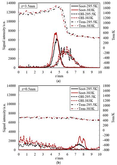
Figure 12.
Experimental soot emission, OH radical and temperature at (a) z = 3.5 mm (free flame zone) and (b) z = 0.5 mm (near-wall flame) for the cold and hot walls.
In the near-wall flame zone, the temperature is very low because of strong heat transfer to the wall, and then the thermal chemical reaction is suppressed. Soot emission and OH radicals will certainly go away in the quenching layer. However, some weak signals from LII and LIF measurement appear visible over a broadened area. Referring to Section 3, the LIF signal near the flame centerline originate from some interference emitted by other species. Surprisingly, in the outside the flame, small soot formation also has been observed close to the wall. One possible reason for soot appearance near the wall is that the spatial distribution of soot particles is determined by the surrounding flow, such as co-flow, in addition to the temperature effect on the chemical formation process.
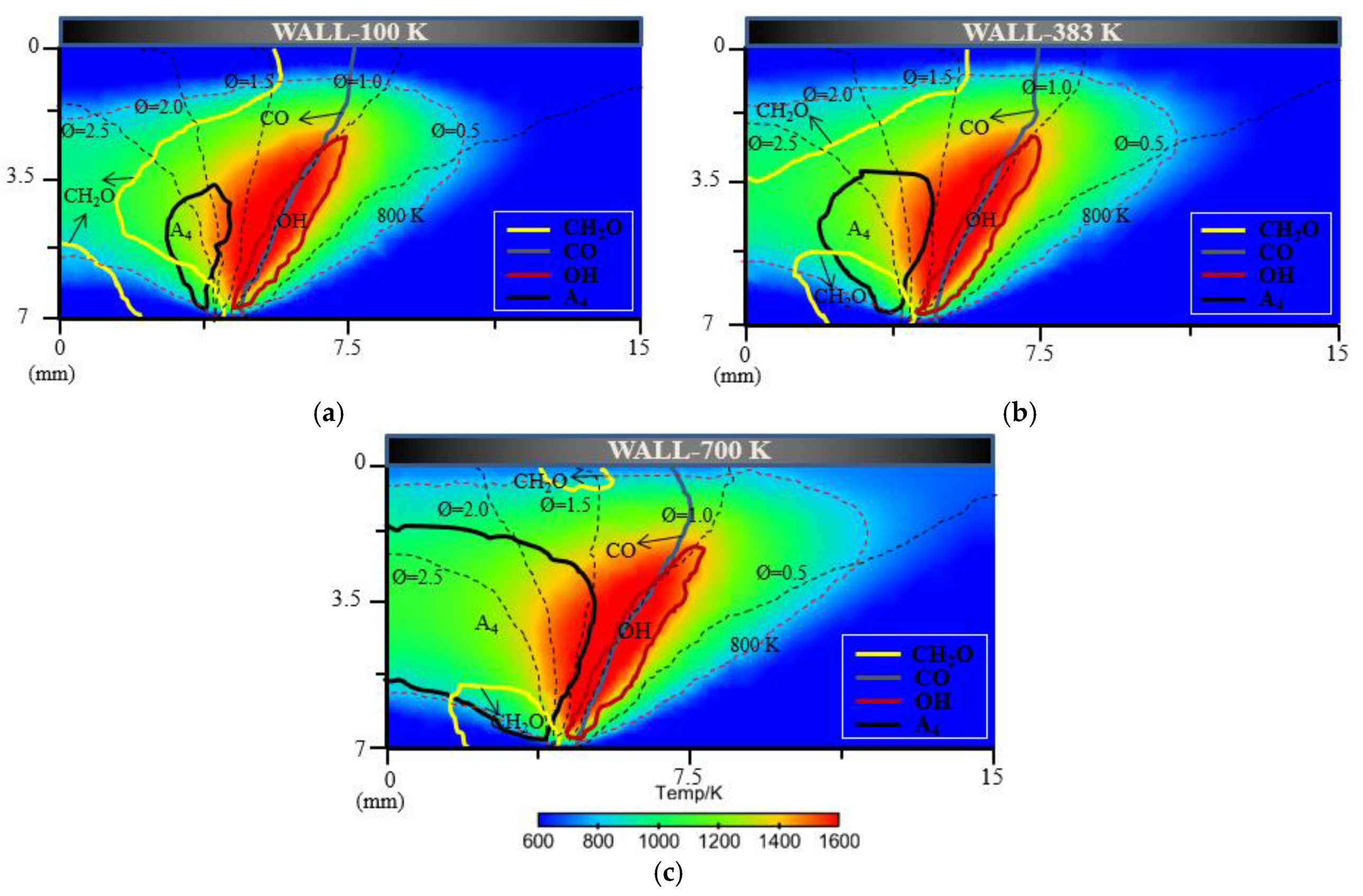
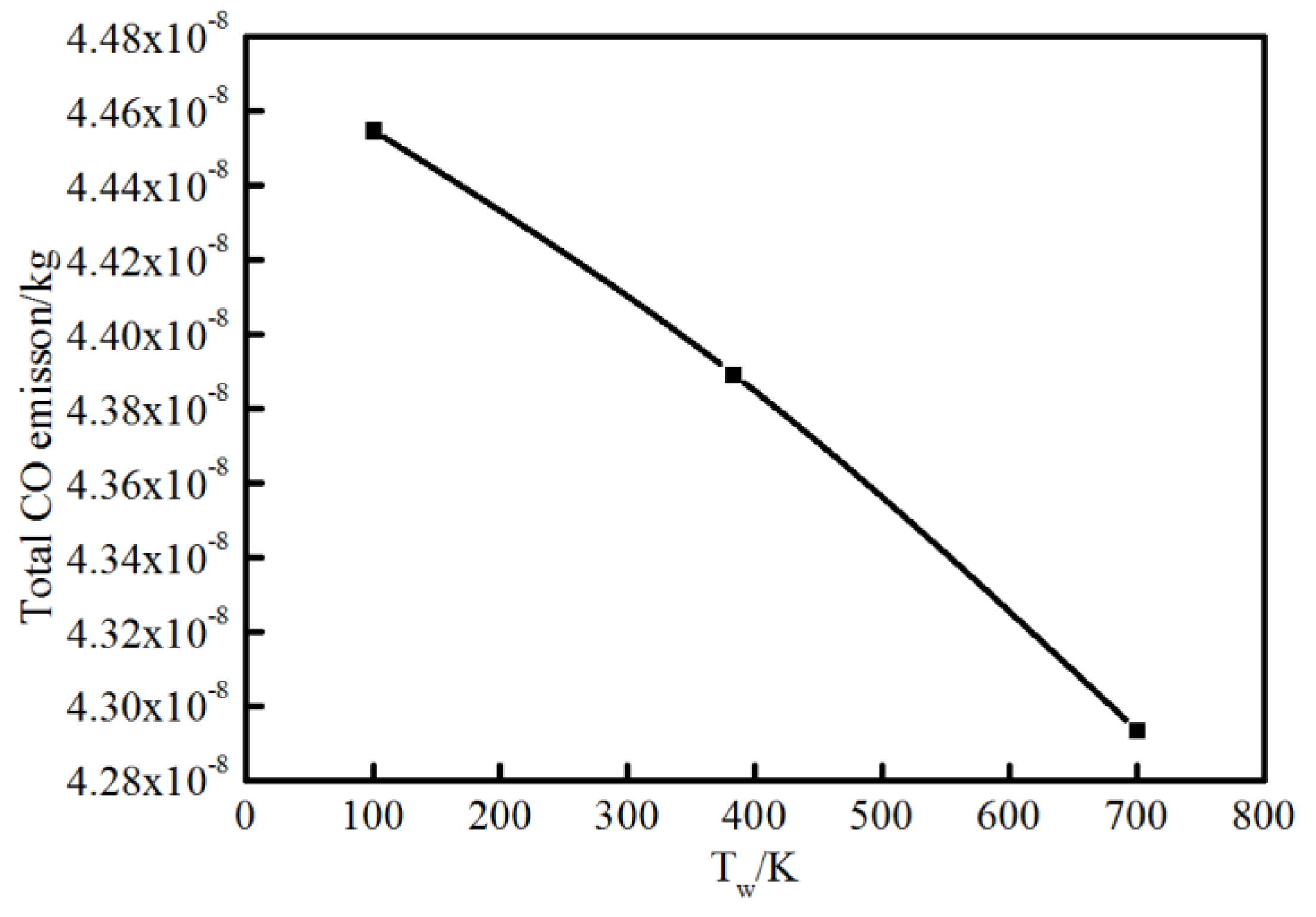
For flame–wall interaction, some emissions (CO, CH2O, HC, etc.) are significant for the evaluation of combustion performance. A CFD simulation coupled with a detailed chemical kinetics mechanism was a natural choice to complement experimental approached to the emission performance near the wall. Additionally, the characteristics of 2D flame structures from simulation could also demonstrate detailed and intuitive information for a further concrete analysis of flame–wall interaction. Figure 13 shows the characteristics of 2D flame structures for different wall temperatures. To investigate the influence mechanism of wall temperature on flame–wall interaction, three wall conditions (100 K, 383 K and 700 K), including extreme cold and extreme hot environments, were selected. The characteristics of 2D flame structures display the main formation areas of CH2O, CO, OH, A4 (pyrene, four-ring aromatic hydrocarbon) on the respective temperature and concentration fields. The respective contour lines of each species in the three conditions represent the same mole fraction. For each enclosed region and area, arrows point to designate the domain where the species concentration is above the certain mole fraction. A temperature contour of 800 K indicates the level of wall quenching. The contour is closer to the surface as wall temperature increases, which points to a smaller quenching layer. The greater quenching distance will cause more CH2O, CO and HC emissions, primarily produced in the low-temperature condition. In these cases, formaldehyde is found mainly in the fuel-rich and cold regions, such as close to the wall and in the preheating zone close to the fuel nozzle. For the colder wall, the area of significant CH2O within the spatial region is more extended than the area for the hotter wall. The obvious difference in area for formaldehyde occurrence exists on the upstream side of the flame and at some distance from the wall. A possible explanation for these findings might be that the heat transfer to the surface accompanying lower temperature retards the onset of the pre-combustion reactions, bringing about formaldehyde formation. Compared with formaldehyde, CO appears visible over a broadened area close to the outer flame where temperature is higher. CO distribution is spatially similar for various wall conditions, while the total CO emission increases as the wall temperature decreases, as indicated in Figure 14. This is attributed to the effect of wall temperature; that is, the heat losses to the cold wall inhibits the reaction path for CO. The gas near the wall is cooled down and further oxidation of carbon monoxide is not possible, which increases the CO mole fraction at lower temperature.

Figure 13.
The characteristics of 2D flame structures for different wall temperatures: (a) 100 K; (b) 383 K and (c) 700 K.
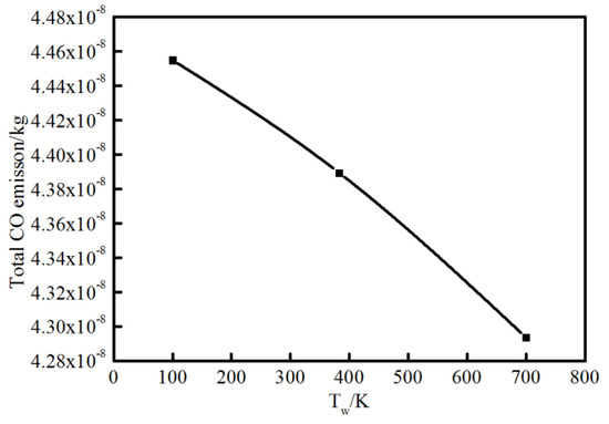
Figure 14.
Total CO emission at different wall temperatures.
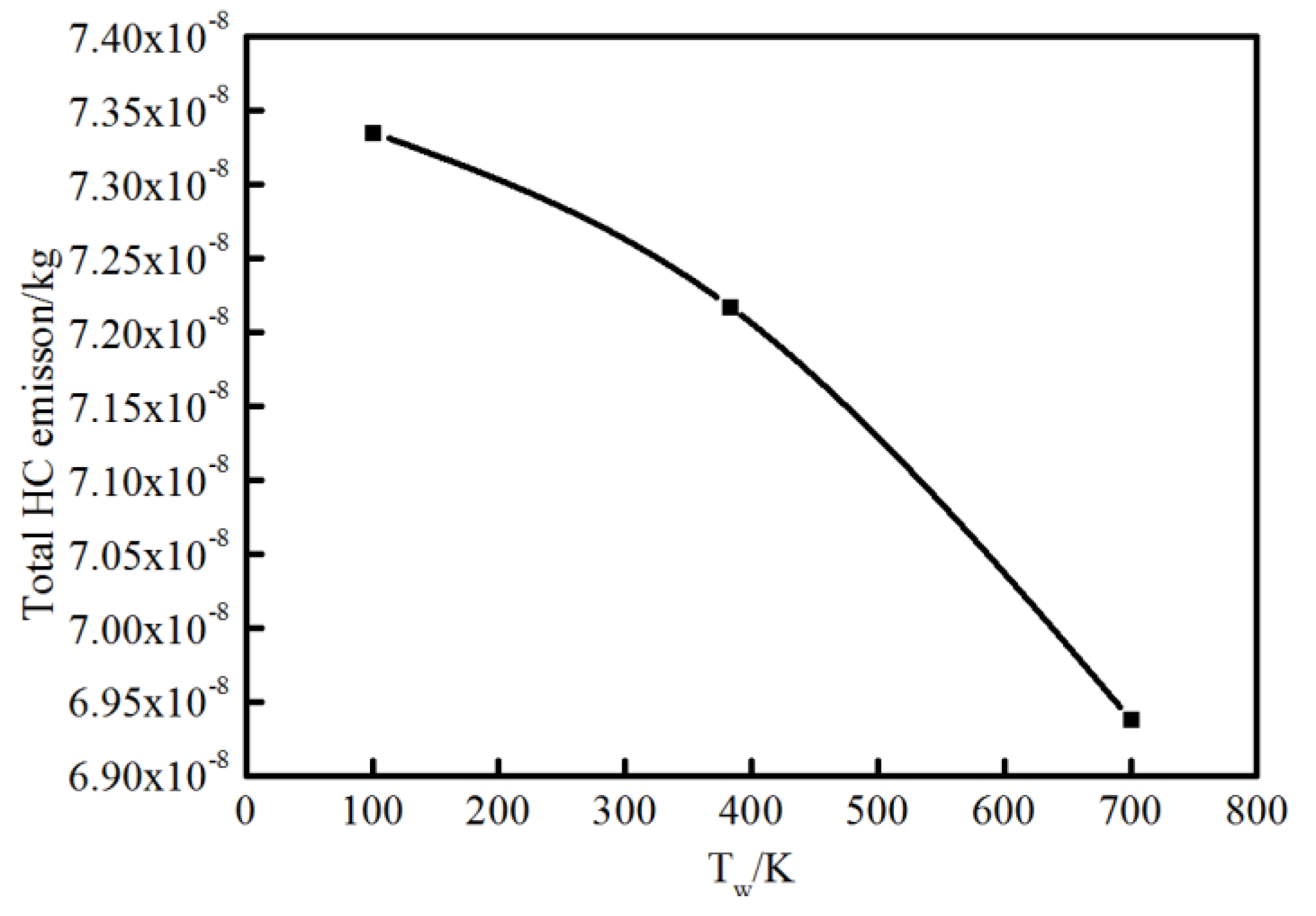
As the vital soot-precursor, A4 is exhibited to predict the soot formation. The chief pyrene formation occurs at slightly higher temperature and rich condition far from the surface, where the equivalence ratio exceed almost 1.5. The overall A4 appears much more and wider because of higher average temperature caused by elevated wall temperature, which is an indication of greater soot emission formation. This result coincides with the experimental soot tendency. For OH, the location is near the stoichiometric condition where the temperature is extremely high, as is also seen using optical diagnostics. Figure 15 indicates the total HC emission with different wall conditions. As stated previously, the colder the wall is, the more HC emission forms.
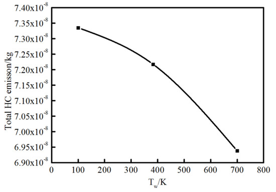
Figure 15.
Total HC emission at different wall temperatures.
5. Conclusions
The role of wall temperature in flame–wall interaction behavior was investigated with an acetylene diffusion flame formed in a head-on quenching type. Direct photography, two-color thermometry, soot-LII, OH-LIF and CFD simulation with detailed reaction mechanisms were employed to find out the influencing mechanism of wall temperature on near-wall combustion performance and emission characteristics. The following conclusions are derived.
According to optical experiments, the high-temperature zone (>1600 K) is in the outer flame, and its area for hot wall becomes wider than that for cold wall. The measured temperature is very low near the cold wall due to the thermal quenching effect and the low-temperature zone (approximately 600 K) is closer to the wall when Tw increases. In spite of some discrepancy between experiments and simulations, the simulated flame structure is similar to the experiment, and this CFD model can simulate the impact of wall thermal on temperature distribution near the wall well.
The simulated results indicate that the temperature near the wall goes up and the wall heat flux decreases with increasing Tw. This leads to a change of quenching distance. The experimental quenching distance decreases from 0.535 mm to 0.426 mm with increasing Tw, from 295.5 K to 383 K. The lower wall temperature results in the greater quenching distance due to the higher wall heat flux.
Through the experiments, high-concentration soot emission is formed primarily near the outer flame, far from the wall where there is a high-temperature and fuel-rich zone. The total soot volume fraction increases from 99.08 ppm to 121.68 ppm with the increasing wall temperature, from 295.5 K to 383 K. OH location is near the stoichiometric condition in the high-temperature zone, which is also revealed in the CFD simulation. An overlapping of the soot and OH signals indicates oxidation of the soot via OH.
By CFD simulation, CH2O, CO and HC emissions are primarily produced in the low-temperature zone and decrease as wall temperature rises. CO appears visible in a wider and higher temperature area than CH2O. A4 appears much more and with a wider area because of the higher average temperature caused by elevated wall temperature, which is an indication of greater soot emission formation. Finally, a diffusion flame–wall interaction structure is proposed to reveal the influence mechanism of wall temperature.
Author Contributions
All authors have worked on this manuscript together and all authors have read and approved the final manuscript. H.L., C.G. and Z.Y. planned and conducted the research works. H.L. and C.G. analyzed the experimental and simulated data. H.L. and C.G. wrote the paper. Y.C. helped to check the English. M.Y. provided useful suggestions and help during the whole work.
Acknowledgments
The authors would like to thank the financial support by the National Natural Science Foundation of China through the project of 91541205 and 91541111.
Conflicts of Interest
The authors declare no conflicts of interest.
Abbreviations
| AMR | Adaptive Mesh Refinement |
| CARS | Coherent Anti-Stokes Raman Spectroscopy |
| CFD | Computed Fluid Dynamic |
| DNS | Direct Numerical Simulation |
| FGM | Flamelet Generated Manifold |
| FWI | Flame–Wall Interaction |
| HOQ | Head-On Quenching |
| ICCD | Intensified Charge Coupled Device |
| LIF | Laser Induced Fluorescence |
| LII | Laser Induced Incandescence |
| PAH | Polycyclic Aromatic Hydrocarbons |
| SWQ | Side-Wall Quenching |
| TP | Two-Photon LIF and Phosphor Thermometry |
| UHC | Unburned Hydrocarbon |
References
- Laget, O.; Muller, L.; Truffin, K.; Kashdan, J.; Kumar, R.; Sotton, J.; Boust, B.; Bellenoue, M. Experiments and modeling of flame/wall interaction in spark-ignition (SI) engine conditions. SAE Pap. 2013. [Google Scholar] [CrossRef]
- Demesoukas, S.; Caillol, C.; Higelin, P.; Boiarciuc, A.; Floch, A. Near wall combustion modeling in spark ignition engines. Part A: Flame–wall interaction. Energy Convers. Manag. 2015, 106, 1426–1438. [Google Scholar] [CrossRef]
- Lakshmanan, T.; Nagarajan, G. Experimental investigation on dual fuel operation of acetylene in a DI diesel engine. Fuel Process. Technol. 2010, 91, 496–503. [Google Scholar] [CrossRef]
- Lakshmanan, T.; Nagarajan, G. Experimental investigation of port injection of acetylene in DI diesel engine in dual fuel mode. Fuel 2011, 90, 2571–2577. [Google Scholar] [CrossRef]
- Fuyuto, T.; Kronemayer, H.; Lewerich, B.; Brubach, J.; Fujikawa, T.; Akihama, K.; Dreier, T.; Schulz, C. Temperature and species measurement in a quenching boundary layer on a flat-flame burner. Exp. Fluids 2010, 49, 783–795. [Google Scholar] [CrossRef]
- Kim, D.; Ekoto, I.; Colban, W.F.; Miles, P.C. In-cylinder CO and UHC Imaging in a Light-Duty Diesel Engine during PPCI Low-Temperature Combustion. SAE Pap. 2008, 1, 933–956. [Google Scholar] [CrossRef]
- Heeger, C.; Gordon, R.L.; Tummers, M.J.; Sattelmayer, T.; Dreizler, A. Experimental analysis of flashback in lean premixed swirling flames: Upstream flame propagation. Exp. Fluids 2010, 49, 853–863. [Google Scholar] [CrossRef]
- Künne, G. Large Eddy Simulation of Premixed Combustion Using Artificial Flame Thickening Coupled with Tabulated Chemistry, 1st ed.; Optimus Verlag: Göttingen, Germany, 2012. [Google Scholar]
- Liu, H.; Ma, S.; Zhang, Z.; Zheng, Z.; Yao, M. Study of the control strategies on soot reduction under early-injection conditions on a diesel engine. Fuel 2015, 139, 472–481. [Google Scholar] [CrossRef]
- Mann, M.; Jainski, C.; Euler, M.; Bohm, B.; Dreizler, A. Experimental analysis using spectroscopic temperature and CO concentration measurements. Combust. Flame 2014, 161, 2371–2386. [Google Scholar] [CrossRef]
- Dreizler, A.; Bohm, B. Advanced laser diagnostics for an improved understanding of premixed flame-wall interactions. Proc. Combust. Inst. 2015, 35, 37–64. [Google Scholar] [CrossRef]
- Boust, B.; Sotton, J.; Labuda, S.A.; Bellenoue, M. A thermal formulation for single-wall quenching of transient laminar flames. Combust. Flame 2007, 149, 286–294. [Google Scholar] [CrossRef]
- Dabireau, F.; Cuenot, B.; Vermorel, O.; Poinsot, T. Interaction of flames of H2 + O2 with inert walls. Combust. Flame 2003, 135, 123–133. [Google Scholar] [CrossRef]
- Wang, Y.; Trouve, A. Direct numerical simulation of nonpremixed flame-wall interactions. Combust. Flame 2006, 144, 461–475. [Google Scholar] [CrossRef]
- Desoutter, G.; Cuenot, B.; Habchi, C.; Poinsot, T. Interaction of a premixed flame with a liquid fuel film on a wall. Proc. Combust. Inst. 2005, 30, 259–266. [Google Scholar] [CrossRef]
- Heinrich, A.; Ganter, S.; Kuenne, G.; Jainski, C.; Dreizler, A.; Janicka, J. 3D Numerical Simulation of a Laminar Experimental SWQ Burner with Tabulated Chemistry. Flow Turbul. Combust. 2017, 1, 1–25. [Google Scholar] [CrossRef]
- Tang, Q.L.; Zhang, P.; Liu, H.F.; Yao, M.F. Quantitative Measurements of Soot Volume Fractions in Diesel Engine Using Laser-Induced Incandescence Method. Acta Phys. Chim. Sin. 2015, 31, 980–988. [Google Scholar]
- Melton, L.A. Soot diagnostics based on laser heating. Appl. Opt. 1984, 23, 2201–2208. [Google Scholar] [CrossRef] [PubMed]
- Hofeldt, D.L. Real-Time Soot Concentration Measurement Technique for Engine Exhaust Streams. SAE Pap. 1993. [Google Scholar] [CrossRef]
- Quay, B.; Lee, T.W.; Ni, T.; Santoro, R.J. Spatially resolved measurements of soot volume fraction using laser-induced incandescence. Combust. Flame 1994, 97, 384–392. [Google Scholar] [CrossRef]
- Chen, B.; Liu, X.; Liu, H.; Wang, H.; Kyritsis, D.C.; Yao, M. Soot reduction effects of the addition of four butanol isomers on partially premixed flames of diesel surrogates. Combust. Flame 2017, 177, 123–136. [Google Scholar] [CrossRef]
- Liu, H.; Zhang, P.; Liu, X.; Chen, B.; Geng, C.; Li, B.; Wang, H.; Li, Z.; Yao, M. Laser diagnostics and chemical kinetic analysis of PAHs and soot in co-flow partially premixed flames using diesel surrogate and oxygenated additives of n-butanol and DMF. Combust. Flame 2018, 188, 129–141. [Google Scholar] [CrossRef]
- Lawrence Livermore National Laboratory, C1-C2 Detailed Mechanism, Version 1.2. Available online: https://library-ext.llnl.gov/ (accessed on 16 November 1996).

© 2018 by the authors. Licensee MDPI, Basel, Switzerland. This article is an open access article distributed under the terms and conditions of the Creative Commons Attribution (CC BY) license (http://creativecommons.org/licenses/by/4.0/).