Abstract
Low-voltage power line communication (LVPLC) medium access control protocols significantly affect home area networks performance. This study addresses poor network performance issues caused by asymmetric channels and noise interference by proposing the following: (i) an improved Q learning method for optimizing the improved artificial LVPLC cobweb, wherein the learning-based hybrid time-division-multiple-access (TDMA)/carrier-sense-multiple-access (CSMA) protocol, the asymmetrical network system, is modeled as a discrete Markov decision process, associates the station information using online trial-and-error learning, builds a routing table, periodically studies stations to choose a better forward path, and optimizes the shortest backbone cluster tree between the central coordinator and the stations, guaranteeing network stability; and (ii) an improved adaptive p-persistent CSMA game optimization method is proposed to optimize the improved artificial cobweb saturation throughput and access delay performance. The current state of the game (e.g., the number of competitive stations) for each station is estimated by the hidden Markov model. The station changes its equilibrium strategy based on the estimated number of active stations, which reduces the collision probability of data packets, optimizes channel transmission status, and increases performance by dynamically adjusting the probability p. An optimal saturation performance is achieved by finitely repeating the game. We present numerical results to validate our proposed approach.
1. Introduction
Aging power grids are being increasingly replaced with infrastructure that includes advanced communication technologies, called “smart grids,” thereby bringing attention to the use of power line communication (PLC) as an appropriate network technology [1]. Smart grids require advanced communication, control, and information technologies to support intelligent applications, such as electronic control, self-healing, and indoor local area network (LAN) services. The success of a smart grid depends heavily on high-speed and reliable data transmission, because some smart grid applications need to be performed in real time. There is no doubt that smart grids will exploit multiple communication technologies to guarantee reliability, and PLC is very attractive as a viable home area networking (HAN) solution, because of its inherent features such as inexpensive installations, the use of existing electrical wiring, broad coverage, and easy scalability.
Power systems generally consist of four parts: generation, transmission, distribution, and consumption. Power is generated and transported at high voltage. It is distributed over regional areas at medium and low voltages (LV) and consumed at LV. In this work, we focus on home area networking technology, which covers LV distribution networks. Broadband PLC (BB-PLC, operating in the 1.8–20 MHz frequency band) is designed to meet the requirements of indoor wired LAN services for residential areas or access network requirements. However, PLC suffers from unpredictable signal-to-noise ratios and bit error rates [2]. Reliable two-way data communication over a multipath fading channel requires robust medium access control (MAC) protocols to overcome these problems. The abovementioned technique is clearly defined in low-voltage power line communication (LVPLC) standards, such as HomePlugAV2, IEEE1901, and PRIME [3,4]. Current research primarily assumes symmetrical channel characteristics and provides relatively little consideration to the effects of asymmetrical channels and impulse noise on the network performance. Therefore, the author considers the abovementioned factors and their similarity to wireless communication at the sharing nature of a common medium to generally improve the network stability and saturation performance.
Recent field tests have revealed a relative drop in performance in one-hop or multi-hop networks when the asymmetric channel factors are considered. Thus, network algorithms play a key role in LVPLC networks [5]. Many algorithms have been improved based on wireless communication networks, and proposed for the LVPLC network. However, all these algorithms are proposed for a specific network scenario; hence, they cannot be easily adjusted for different environments. In [6], the author noted that stations rebroadcast the received frames by adopting a flooding algorithm, which causes many collisions and becomes inefficient as the station density increases. Another study [7] proposed an improved algorithm for controlling the number of broadcasts made by a station. However, the researchers did not consider how retransmission by a given station would affect message reception by neighboring stations. In [8], adopting a higher data rate may also lead to more hops from source to destination and weaker multi-hop network connectivity, which in turn may result in throughput and delay degradation. This dilemma provides the motivation for the current study on the topology control algorithm. Reference [9] shows that providing the right infrastructure for connecting these PLC stations will be a major requirement. For home applications, this infrastructure must be easy to set up, maintain, and must perform well. Homeowners are generally not network experts, and a typical high-performance network is too complex for casual daily usage. The study [10] proposes a solution for home automation and high data rate (theoretical maximum physical rates up to 1 Gbps) local networks by applying the PLC. As the number of stations increases, interference among stations occurs and causes instability. There is a need to propose an improved control mechanism at the MAC layer. Reference [11] proposed an artificial cobweb network algorithm. However, this type of algorithm depends to some extent on the central coordinator (CCo). In Reference [12], the author proposed an improved ant colony network algorithm, which easily reaches the local optimal. Through the abovementioned analysis, the author considered it necessary to study the flexible network topology control method and consider multiple metrics, because the network topology and channel parameters vary for different scenarios, to guarantee overall network performance.
The topology and the technical characteristics of the electricity network strongly affect communication performance. Therefore, analysis of the performance of PLC networks is very important, and can be assessed analytically through simulations to obtain a relatively optimal performance [13]. Research focusing on saturation performance analysis and channel access design has been under-explored because of stability issues. In [14], an adaptive contention window mechanism in the MAC protocol of HomePlug1.0 was proposed to improve performance given the number of known active stations within the network. However, stations do not have exact knowledge of this information. This assumption was therefore unrealistic. Yoon et al. [15] proposed a heuristic throughput optimization method that can run without knowing the exact number of contending stations. These investigations assume that the communication channel is ideal (i.e., no transmission error due to the bad channel). This is also not a valid assumption in real LVPLC network environments. In [16], the author ignores the noise factor, which seriously degrades performance, especially when each station’s load approaches its saturation state. In addition, the transmission error probability was not constrained in the throughput model. The authors in [17] proposed a relatively simple learning method for relay selection in a cooperative network and the throughput performance was shown. However, most works aimed at optimizing the throughput performance while ignoring the access delay and transmission efficiency performance. Reference [18] provided an optimal solution for globally obtaining maximum throughput, but did not consider the effects of individual selfishness. In [19], the author proposed game-theory-based carrier-sense multiple access (CSMA) for the wireless network. However, asymmetry was not accounted for in the model, and the researchers did not further investigate access delays. In [20], the author analyzed several access control models based on game theory, which affected performance because of the complex calculations required.
Motivated by the abovementioned studies, we propose herein an improved adaptive p-persistent CSMA-protocol-based dynamic game to guarantee an improved artificial cobweb saturation performance in asymmetric-channel and noise-interference environments. Overall, our contribution can be summarized as follows:
- (i)
- We use a learning-based hybrid time division multiple access CSMA (TDMA–CSMA) protocol as the control policy and apply the finite state machine (FSM) to show the stations’ network state. We propose an improved Q learning method to network the improved LVPLC artificial cobweb. The station is treated as an agent, while the network system is modeled as a discrete Markov decision process. The station uses the local path information in the routing table, periodically studies, and online bi-directional learns the link information. In the design of the reward function, we take account of the available link quality and the number of hops. Stations choose the optimal shortest backbone cluster tree to transmit the beacon slot between the CCo and the stations and achieve a dynamical self-organized network.
- (ii)
- We propose using the improved adaptive p-persistent CSMA-based dynamic game theory to optimize the saturation performance of the improved LVPLC artificial cobweb and address the problem of how to guarantee the saturation performance under unknown numbers of active stations. Each station independently estimates the number of competitive stations using a hidden Markov model (HMM), adopts the optimum probability for sending the data packets, and achieves performance optimization.
This paper is organized as follows: Section 2 presents the low-voltage distribution network topology; Section 3 describes the LVPLC network scheme; Section 4 describes the incompletely cooperative dynamic game model that optimizes the saturation throughput and the access delay performance; Section 5 presents some numerical simulation results not previously reported; and Section 6 draws the conclusions.
2. Low-Voltage Distribution Network Topology
This section describes the physical topology of the low-voltage distribution network and the logical topology of the communication system.
2.1. Physical Topology of the Low-Voltage Distribution Network
The LV network represents a simple tree topological structure, and the channel frequency responses between pairs of stations are obtained with a bottom-up channel generator [21], although it was generally applied to in-home networks, as depicted in Figure 1. The signal attenuation among the A, B, and C phases is very large for the secondary side of the transformer in the three-phase power distribution grid [22]. The end customers are represented as an intelligent device in each phase. Devices in the same vicinity are connected to the three different phases for load balancing. Without phase coupling, each of the A, B, and C phases of the three phases are parallel and relatively independent; therefore, this study establishes a single-phase power distribution network based on the tree-like physical topology of a low-voltage distribution network.
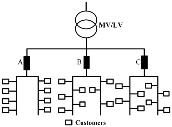
Figure 1.
Typical topology model of the low-voltage distribution network.
2.2. Communication Logical Topology of the LVPLC
Using the tree-like physical topology structure as a basis, we must build a logical topology for our communications to improve network stability and robustness. The LVPLC logical topology is composed of a CCo, a repeater, and a terminal. However, the stations are switched in and out as required, and changes occur in both operating and channel states, directly leading to logical topology changes for the LVPLC network. An improved artificial cobweb topology in the LVPLC network is used to improve stability performance.
3. LVPLC Network Scheme
3.1. Network Problem Description and Modeling
3.1.1. Network Problem Description
Inspired by spider webs in the natural environment, Reference [23] analyzed logical topology processes for a single-layer cobweb topology. This process cuts useful communication links to improve stability. This section describes this improved artificial cobweb logical topology. The stations may not form a ring network in the improved cobweb topology compared with the original cobweb (Figure 2). The critical issues encountered in networking the improved artificial cobweb are as follows: (1) the stations are peer to peer, and a method must be developed to auto-select the CCo and proxy in the network; (2) an increased probability of frame collisions, which causes network instability, is observed because of the effects of hidden stations; and (3) the stations are far from the CCo because of the one-hop or multi-hops, and the overall network performance is poor. To address these problems, the improved artificial cobweb consists of a backbone cluster tree network and a neighbor network. The backbone cluster tree network (objective function) is composed of several shortest dynamic random links from the CCo and proxy to terminals.
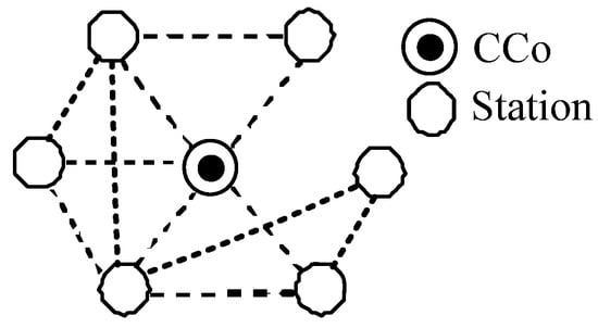
Figure 2.
Improved artificial cobweb.
3.1.2. Network Objective Function
Network optimization is a typical multi-constrained and nonlinear optimization problem. The LVPLC network is modeled as a non-negative weight-directed graph where denotes the set of CCo values and stations ; denotes the set of directed and no-loop links; and denotes the set of non-negative weights, whose value dynamics change, showing the link connection state.
The objective function minimizes several dynamic random shortest paths from CCo to stations in the graph . Assuming that the CCo is O; the destination station is D; the proxy set is ; and the shortest path of the station set is , the elements in are represented as in order in the shortest path. The objective function of the shortest path can be expressed as:
s. t.
Equation (1) shows the objective function. Formula (2) shows the constraint conditions of the CCo, proxy, and destination station. Equation (3) shows the definition of the decision variables xij. If the link exists, xij = 1; otherwise, xij = 0. Equation (4) shows a necessary constraint on the proxy. Equation (5) indicates that the proxies are divided into w classes. Equation (6) indicates that there is no loop between every class. Equation (7) indicates that at least one station in each class is stations. Equation (8) denotes the grouped and order-preserving stations shortest path, which in turn, passes stations . We propose an improved Q-learning method for the LVPLC network for the grouped and order-preserving proxy shortest paths.
3.2. Improved Q Learning Approach in LVPLC Network Scheme
3.2.1. Improved Q Learning Model
Q learning Mathematic Model
Reinforcement learning (RL) methods are used to control data packet delivery decisions and improve network stability. They consist of three abstract learning algorithm events: (1) a station observes the state of the environment, generates a reinforcement signal, and selects an appropriate action; (2) the environment generates a reinforcement signal and transmits it to the station; and (3) the station employs the reinforcement signal to improve its subsequent decision. Therefore, a station requires information about the state of the environment, reinforcement signals from the environment, and a learning algorithm (Figure 3).
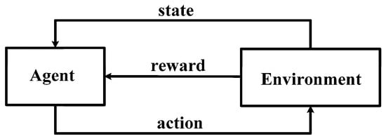
Figure 3.
RL model.
A number of RL algorithms, such as Q-learning and temporal difference learning, have been used. Q-learning is a recent form reinforcement learning that does not need a model of its environment and works by estimating the values of state-action pairs. It learns behavior through trial-and-error interactions with a dynamic environment, and has been employed for path selection [24]. The algorithm maintains a Q-value Q (s, a) in a table for every state–action pair. Let st and at denote the reinforcement signal generated by the environment for performing action at in state . When the station receives reward rt+1, it updates the Q-value corresponding to state st and action at as follows:
where r (0 ≤ r ≤ 1) is the discount factor, and (0 ≤ ≤ 1) is the learning rate. The return is deterministic when . Equation (9) is then changed as follows:
The agent selects the action with the highest Q-value, except when making an exploratory move. The state transition model is unknown in our problem; hence, we are motivated to use the model free Q-learning algorithm idea in the LVPLC network.
Improved Q-Learning Mathematic Model
In reference to the core ideas of the Q algorithm, this study probes deeply into the following problems: (1) how to achieve bidirectional learning among stations while ensuring state/action sets and (2) how to model the reward function in a complex channel environment.
We map herein the state, action, and reward functions for the multi-constrained improved Q-learning to the LVPLC network.
● State
The general finite state machine (FSM) model shows the states of stations in different network stages, including the initial state (INIT), uncoordinated CCo (UC_CCo), uncoordinated STA (UC_STA), the coordinated CCo (C_CCo), and coordinated STA (C_STA). The C_CCo and C_STA show the stability states of stations.
● Action
Station states evolve from instability to stability via action triggers. The station selects an action under control policy , such as sending/receiving the beacon. It defines all actions as set A. The action in set A can be divided into feasible action and infeasible action The uplink/downlink communication success ratio (csr) threshold value can be defined as . The action is shown as follows when the current csr is greater than the threshold value :
The destination stations send the Acknowledgment (ACK) to the source station and avoid the frame retransmission when the destination stations successfully receive the frame.
● Reward function
When stations meet the requirements of the communication threshold condition, indicates the reward after stations associate the network through trial-and-error interactions with a dynamic environment:
where denotes the link weight when station i receives the data frame; is the link weight when station j sends the data frame; and denotes the hops between stations i and j. These metrics (link quality, the number of hops) are considered jointly in the reward function, and can reflect the dynamic characteristics of the network. The greater the value of the reward, the stronger the learning trend.
● Q value update rule
The forwarding Q-learning in the asymmetric channel environments is from the CCo to the terminals. The backward Q-learning is from the terminals to the CCo. This study explains the forward Q-learning mechanism. The CCo obtains the new associated stations’ information by gathering proxies and provides immediate reward to the new stations when the csr is greater than the uplink csr threshold . The CCo puts the new associated stations into the routing table, dynamically updates the routing table information, and finishes the forwarding link storage. The stations choose the next hop to continue networking by routing table lookup. The whole stations associate in the network, and the network finishes. The CCo’s Q table information is updated as follows:
where is the present uplink csr.
This study illustrates the backward Q-learning mechanism. The new associated stations obtain terminal equipment identifiers (TEIs) by the CCo allots and stores the link to the CCo when the csr is greater than the downlink csr threshold . The stations’ Q table information is updated as:
where is the present downlink csr.
3.2.2. Improved Q-Learning Algorithm in LVPLC Network
We describe several assumptions and notations for the backbone cluster tree analysis to facilitate scheme discussion.
Assumption
The n (n > 1) stations are connected with the same medium and physical links, and the following assumptions are made:
- Only the MAC address is unique to the station.
- Each station communicates with at least one other station when the communication environment of the channel is good.
- The CCo does not repeatedly assign and then reclaim TEIs.
- No more than three retransmission times are present.
- The electrical signal transmission time is neglected in the copper medium.
Network Information Table
This study proposes the usage of three important tables (i.e., routing table, topology table, and neighbor table) to store the stations’ information during the dynamic network process.
The routing table (Q-table) is used to store the link information from the origin address to the destinations. Each station maintains a routing table. The table includes the hop count, original address, the next hop address, and destination address. According to the topology control strategy, stations put the next hop information into the network frame and send it to the destination station by broadcasting way. If the other stations receive the frame and find the address information to be different from their addresses, they discard it and avoid network loop. The topology table is used to store all the stations’ connectivity relationships, and only the CCo stores this table. The neighbor table is used to store the stations’ neighbor information. The information represents the stations’ connectivity relationships. Each station also maintains a neighbor table.
Improved Q-Learning Network Mechanism
Typical CSMA and TDMA mechanisms are extensively studied. The CSMA suffers from heavy interference because of hidden terminals, and often exhibits a large delay. The TDMA has practical difficulties achieving an accurate time synchronization. Achieving such synchronization via beacon exchanges is generally expensive. Therefore, we propose an online bi-directional improved Q-learning network mechanism based on the hybrid TDMA–CSMA protocol. The structural properties of the LVPLC networks are relatively complex. This study introduces a small number of topological measurements to compute the station importance (i.e., centrality degree, closeness degree, betweenness degree, clustering coefficient, and average shortest path [25]). The value of the closeness degree is the reciprocal of the average distance between each station pair:
where is the closeness centrality of station v, and is the distance of the shortest path connecting station v and j.
The relative betweenness centrality of measures a station v that lies on the shortest path between any pair of stations passing through a specific station:
where is the total number of shortest paths from station i to j, and is the number of shortest paths from station i to j passing v.
The clustering coefficient of station i is calculated as:
where is the number of links between stations . The average path is calculated as follows:
where is the distance between i and j.
An improved Q-learning mechanism based on the hybrid TDMA + CSMA (control policy) mechanism is described as follows:
- Auto selection of CCo: All stations are powered on at the same time, and their parameters are initialized. After 5 s of silence, the station with the shortest delay randomly sends the SELECT_CCO beacon frame to the other stations in the radius of communication. The receivers reply to the sender with an ACK after waiting for the response inter frame space (RIFS). The CCo selection is a success if the station successfully receives the ACK. The state machine of the station becomes UC_CCO from INIT. The state machines of the other stations become UC_STA from INIT. If the CCo selection fails, the abovementioned mechanism is repeated until the selection is successful.
- CCo q first allots a beacon slot for itself, as depicted in Figure 4a. In the SLOT0, CCo q broadcasts a beacon frame to the other stations. The other stations delay for a short and random period of time. They then self-schedule the ASSOC.REQ frame, access the channel by CSMA, and send it to CCo q. A frame collision occurs if at least two stations simultaneously access the channel to send a frame. The stations again delay for a short and random period of time and sense the channel state. The station retransmits the ASSOC.REQ frame to CCo q if the channel is idle.
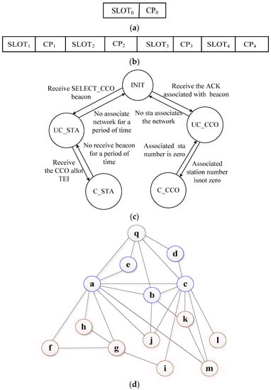 Figure 4. Network beacon slot, FSM and topology diagram. (a) CCo beacon slot; (b) Stations’ beacon slot; (c) Finite state machine; (d) LVPLC stereoscopic network topology.
 - CCo directly replies to the ACK to guarantee the frame transmission success, which puts the stations in the routing table, learn the link to stations, and completes the forward path learning. Station a, which has received the ACK, establishes a connection with CCo . Similarly, stations c, e, d, and b establish a connection with CCo . When SLOT0 ends, CCo broadcasts the ASSOC.CNF frame to the stations in the convergence period 0 (CP0). Stations c, e, d, and b receive TEIs. These stations then place CCo in the routing table, learn the link to , and complete the backward path learning. Stations a, c, e, d, and b have associated the network. The state machine of CCo evolves C_CCO from UC_CCO. The associated station state machine evolves C_STA from UC_STA.
- CCo re-allocates the beacon slot to reduce the maintenance overhead and force as many stations as possible to associate the first layer of the network. CCo repeats the abovementioned mechanism if new stations are available to associate; otherwise, the first layer cluster tree completes the network.
- CCo allocates a beacon slot to four stations every beacon period, as depicted in Figure 4b. If the number of stations is greater than four in the first layer, CCo allots a beacon slot to the remaining stations in the next beacon period. Let us take stations a, c, e, d, and b as examples to explain the network process for the remaining beacon stations. If station a obtains the first beacon slot, it sends a beacon frame to the other stations by broadcasting it in SLOT1. If the associated stations receive the beacon frame, they place station a in a neighboring table and establish a link. If the stations that do not associate the network receive the beacon frame, they delay for a short and random period of time, then self-schedule the ASSOC.REQ frame, access the channel by CSMA, and send it to station a. Station a replies to the ACK after waiting for the contention inter frame space (CIFS), such as that for station . The other network mechanisms are similar to f. Station a sends the ASSOC_ALL.REQ frame to CCo in the CP1 when SLOT1 ends.
- CCo replies to the ACK, puts the new associated stations into the routing table, learns the link to the new associated stations, and completes the forward path Q-learning to the new associated stations. CCo broadcasts the ASSOC_ALL.CNF frame to a. Subsequently, a replies to ACK and broadcasts this frame. The new associated station obtains the TEI, puts station and CCo into the routing table, and completes the backward path Q-learning. Station a becomes the proxy, and stations j, h, g, f, i, l, k, and m become the associated station. The state machine evolves C_STA from UC_STA. The second layer completes the network, as shown in Figure 4c,d.
4. Network Performance Optimization Based on Dynamic Game Theory
We propose using the improved adaptive p-persistent CSMA game optimization method to improve the saturation throughput and access delay performance of the LVPLC improved artificial cobweb.
4.1. Network Performance Model
The following assumptions and notations were used for the performance model analysis.
4.1.1. Assumptions
- The load impedance matches the output impedance in the network.
- A single contention domain with n stations () exists.
- Data packets are of a constant length L.
- Each station always contains data packets in the transmission buffer, and packets are never discarded until a successful transmission.
- The stations do not use request-to-send (RTS) and clear-to-send (CTS) handshake mechanisms.
- The communication distance of the stations is constant at a certain time scale.
- Propagation delays are much shorter than the slot time, and are, therefore, neglected.
4.1.2. Network Saturation Performance Model
Stations send data packages using static p-persistent CSMA, which is relatively simple for network operations. Congestion is also not considered. Stations monotonically send data packets based on the p-persistent CSMA, which has a low bandwidth utilization.
The bandwidth utilization is expressed as follows:
where B denotes the communication bandwidths. The saturation throughput is expressed as:
where denotes the average packet length; is the probability of at least one transmission occurring in the considered slot time; is the probability that a transmission will be successful; and are the average times that the channel is sensed to be busy because of either a successful transmission or a collision, respectively; and denotes the duration of an empty slot time. In terms of , these are:
is a strictly concave function that changes with probability when the station numbers are greater than one. Refer to the parameters in Table 1, which are depicted in Figure 5.

Table 1.
Network parameters.
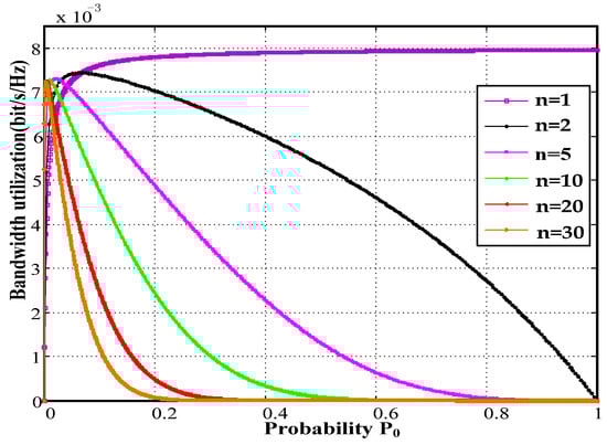
Figure 5.
Relationship between bandwidth utilization and probability p0.
The maximum bandwidth utilization reaches 0.8% bit/s/Hz at a PHY of 1 Mbps for a single station accesses channel. The collision probability also increases with an increasing number of stations. The bandwidth utilization of a single load is 1.1 times the maximum load.
4.1.3. Maximum Saturation Performance
Take the derivative of Equation (19) with respect to p0 to maximize bandwidth utilization. Setting it equal to zero, we obtain the optimal approximate probability solution as follows:
The data packet collision optimal probability is:
Referring to and , the optimal collision probability limit value is calculated when the number of stations approaches infinity:
The stations send the data packets by , reduce the collision probability, and maximize the bandwidth utilization. However, channel asymmetry and noise interference are not considered. In addition, the performance is affected by selfish stations. Inspired by the game theory, this study proposes an improved adaptive p-persistent CSMA-based dynamic game for improving the network saturation performance.
4.2. Performance Optimization Model Based on Game Theory
The competitive channel process for the stations is modeled as an incomplete information dynamic game model. Station dynamics are used to estimate the numbers of active stations using the HMM algorithm. Nash equilibrium (NE) solutions are obtained; bandwidth utilization is achieved; and access delays are optimized. The NE solutions are the optimal channel access probabilities of the stations .
4.2.1. Performance Optimization Theory
Time is divided into a number of discrete time slots. For a given slot, the stations sense the channel before sending data packets by probability p. If the channel is busy, the stations defer data packet transmission until the next time slot. If a channel is sensed to be idle, the stations send data packets to the other stations by . The receiver replies to the ACK via . If more than two stations send data packets at the same time, the collision causes a communication failure. The HMM is used to dynamically estimate the number of competitive stations and compute . This process is finitely repeated to obtain the optimal access probability for achieving optimum performance.
4.2.2. Improved Bandwidth Utilization Model
Suppose that the sender and the receiver send data packets with probabilities , respectively. The station sends the successful probability of the data packet in any slot as follows:
The remaining (n − 1) stations send the successful probability of the data packet:
The bandwidth control ratio factor is defined as:
We obtain the relationship between as follows:
The station sends the successful probability sum of the data packet:
where denotes the probability of the frame errors caused by noise interference and channel fading and depends on the data packet length, transmission rate, and bit error rate in the PHY layer; is the frame error rate (FER) for the data frame; is the FER for the ACK frame; and L_ack denotes the length of the ACK.
The idle probability is given by:
The collision probability is given by:
The improved bandwidth utilization utility model is given by:
The improved bandwidth utilization is maximized when the following quantity is minimized:
Taking the derivative of Equation (39) with respect to and setting it equal to zero, we obtain:
We obtain the following equation after some simplifications:
We obtain the following by substituting Equation (31) in Equation (41):
If , then
This equation is expressed as:
We obtain the only solution to Equation (44) from the Morigane formula, then obtain when is given.
4.2.3. Improved Saturation Access Delay Model
We compute the saturation access delay D in the asymmetrical channel as follows:
The access delay D consists of four parts: (1) denotes the time for a successful transmission; (2) represents the average time the channel is sensed to be busy because of a successful transmission by other stations; (3) represents the average time a channel is sensed to be busy because of collisions; and (4) denotes the total time of idle slots, including the total back-off time of successful transmissions and collisions by each station.
We obtain and compute its three parts according to Equation (23). In the interval of two continuous successful transmissions by a station, the time for successful transmission by each other station is where is the number of successful transmissions by other stations. We assume that all stations are within the communication range of one another, and can fairly share the channel. For a sufficiently long period of time, each station successfully sends data packets with the same probability. Hence, during the interval of two continuous successful transmissions in this station, each other station must have a successful transmission. If n is the total number of stations, then we have . We subsequently obtain:
Let be the count of continuous collisions giving us:
The mean of is
Considering the overall network, continuous collisions are observed during the period of time between two random continuous successful transmissions. According to the above-mentioned analysis, n successful transmissions are observed during time D; thus, we obtain:
Let be the count of continuous idle slots in a back-off interval. The probability that is a random integer can be written as follows:
The mean of is
A back-off interval can be found before each successful transmission or collision; hence, n successful transmissions and collisions exist during time D.
The total time of the idle slot is
4.3. Improved Performance Optimization Model Based on HMM Algorithm
Saturation bandwidth utilization and access delays are sensitive to access probabilities. Access probabilities are relevant to the number of active competitive stations. The stations cannot directly obtain the number of competitive stations. They only rely on themselves to judge channel states, dynamically sense the channel decision results of competitive stations, and obtain the number of competitive stations. This study uses HMM to dynamically sense the number of competitive stations in the game process.
4.3.1. Channel Model
The channel behavior follows a two-state Markov chain with idle () and busy () components, whose one-step transition probability is depicted in Figure 6.
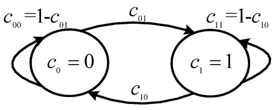
Figure 6.
Markov channel model.
We obtain the solutions of Equation (53) as:
The steady-state probabilities can be calculated from the Markov convergence theorem. Probabilities are used in the dynamic game of the hidden Markov prediction model.
4.3.2. Active Number Dynamic Estimation Based on the Hidden Markov Model
The HMM produces relatively more accurate predictions than the other methods. The HMM estimates station channel decision results through the maximum a posterior (MAP). More accurate channel access information is obtained for the competitive stations when the HMM is combined with game theory mechanisms. Stations adopt appropriate access strategies, and the performance is optimized.
The elements of an HMM are defined as .
- The initial probabilities that stations will judge the channel state .
- The transition probabilities between hidden states with , . indicates the probability that a hidden state will transition at time to another hidden state at time .
- The emission probabilities of the symbols in each hidden state are (i, k = 0, 1), where . bi (k) shows the probability of transition from a hidden state to the observed state .
The basic principle is that the station calculates the prior probability using the posterior probability for the last (t − 1) slot and computes the posterior probability from the observation symbol in the t slot as follows:
where:
Expression is calculated from Equation (56) when is known. Channel state is the current station that estimates competitive stations at time t. It is computed by At the start of the time slots, if station x plays an online game and estimates that the result of the game is one by adopting HMM, the current station saves the results in game set (). Probability is obtained when the current station obtains the game results. Finally, the optimal saturation performance is calculated.
5. Simulation Results
This section discusses the network simulation, saturation performance simulation results in the asymmetric channels, and noise interference communication environment.
5.1. Network Simulation Results
Simulation Environment and Results
Programs such as SimPowerSystems and Matlab/Simulink can be used to simulate a power system distribution network. OMNeT++ and NS-2 are among the most popular tools used to simulate a communication network. In this work, co-simulation platforms designed for controlling information exchange between power and communication software tools can be used. Therefore, we study the LVPLC dynamic self-organization network in the simulation environment of OMNeT++4.0.
Specifically, 30 terminal stations are placed in an 800 800 m2 home local area on the secondary side of the any one phase power distribution grid. This study designs a typical physical topology and a logical communication topology, which are shown in Figure 7a,b, respectively. In Figure 7a, the distance between the neighboring stations is approximately 20 m. The polygonal line symbol shows a line that is 150 m long. Stations communicate with each other within a 200 m range. Outside this range, the stations cannot communicate effectively. Therefore, the logical communication topology can be obtained as shown in Figure 7b. The red station depicts the CCo, while the blue stations present the proxies and terminal stations. The station that uses the contour dotted line shows the new associated stations. Table 1 lists the network’s actual measured parameter.
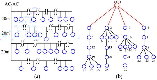
Figure 7.
Typical scenario topology. (a) Typical scenario physical topology; (b) Typical scenario logical topology.
Figure 8a–c shows the topology structure after network in the asymmetric/symmetric channel. The channel asymmetric properties influence the topology structure. Some parts of the stations’ topology measurement (distribution of distances, closeness centrality, and betweenness centrality) are similar to some extent.
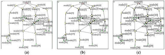
Figure 8.
Improved LVPLC artificial cobweb topology. (a) Topology in the uplink/downlink csr of 96% and 93%; (b) topology in the uplink/downlink csr of 93% and 96%; and (c) topology in the csr of 96% for the symmetric channel.
The node[0], node[2], and node[8] measurement results are presented in Table 2 to quantitatively demonstrate the importance of the stations.
Table 2.
Nodes’ measurement comparison results.
Average Throughputs and Average End-To-End Delays
We simulated the stations (i.e., node[0], node[2], and node[8]) with respect to the average throughputs and the average end-to-end delays to demonstrate the effects of asymmetry on network processes (Figure 9 and Figure 10). We focus on the maximum values, minimum value, and average value to the curve. First, we compare the results of the average throughput of the CCo (node[0]) in the symmetrical/asymmetrical channel environments (Figure 9a). Compared to the symmetric channel-based Q-learning featuring a success ratio of 96%, the proposed method achieves a maximum value of 0.004% less and a minimum value that is basically the same, while raising the average by 0.11% under the traffic environment of uplink 96% success ratio and 93% downlink success ratio. We can reduce the maximum by 0.77%, increase the average by 1.2%, and basically keep the minimum to the same level using the proposed approach instead of the Q-learning under the circumstances of uplink 93% success ratio and downlink 96% success ratio. Second, we explain the comparison results of the average throughput of node[2] (Figure 9b). Compared to the symmetric channel-based Q-learning featuring a success ratio of 96%, the proposed method achieves a minimum value of 6.4% less and a maximum that is basically the same, while reducing the average by 5% under the traffic environment of uplink 96% success ratio and a 93% downlink success ratio. Similarly, we can reduce 0.77% at a maximum, increase the 1.2% on the average, and basically keep the maximum to the same level using the proposed approach instead of the Q-learning under the circumstances of uplink 93% success ratio and downlink 96% success ratio. Finally, we explain the comparison results of the average throughput of node[8] (Figure 9c). Compared to the symmetric channel-based Q-learning featuring a success ratio of 96%, the proposed method achieves a maximum value of 3% less and a minimum that is basically the same, while reducing the average by 0.87% under the traffic environment of uplink 96% success ratio and a 93% downlink success ratio. We can reduce 1.5% at a maximum, increase the 0.87% on the average, and basically keep the minimum to the same level using the proposed approach instead of the Q-learning under the circumstances of uplink 93% success ratio and downlink 96% success ratio.
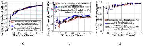
Figure 9.
Node simulation results for the average throughput. (a) Average throughput for node[0]; (b) average throughput for node[2]; and (c) average throughput for node[8].
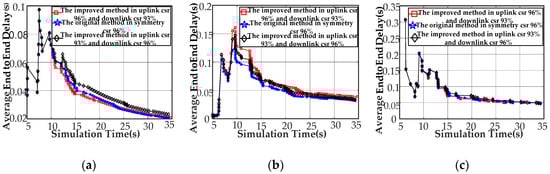
Figure 10.
Node simulation results for the average end-to-end delay. (a) Average ETE delay for node[0]; (b) average ETE for node[2]; and (c) average ETE for node[8].
We explain the results of the average end to end delay of CCo (node[0]) (Figure 10a). Compared to the symmetric channel-based Q-learning featuring a success ratio of 96%, the proposed method achieves a minimum value of 1.6% less and a maximum basically the same, while reducing the average by 1.5%, under the traffic environment of uplink 96% success ratio and 93% downlink success ratio. We can reduce the 12.3% at a maximum, increase the 6.6% on the average and basically keeps the minimum to the same level using the proposed approach instead of the Q-learning under the circumstances of uplink 93% success ratio and downlink 96% success ratio. Next, we explains the comparison results of the average end to end delay of node[2] (Figure 10b). Compared to the symmetric channel-based Q-learning featuring a success ratio of 96%, the proposed method performs about 25.7% above maximum value and a minimum basically the same, while increasing the average by 21% under the traffic environment of uplink 96% success ratio and 93% downlink success ratio. Similarly, we can reduce the 14.6% at a maximum, increase the 8.7% on the average and basically keeps the minimum to the same level using the proposed approach, instead of the Q-learning under the circumstances of uplink 93% success ratio and downlink 96% success ratio. Finally, this paper explains the comparison results of the average end to end delay of node[8] (Figure 10c). Compared to the symmetric channel-based Q-learning featuring a success ratio of 96%, the proposed method performs about 5.3% above maximum value and a minimum basically the same, while reducing the average by 21% under the traffic environment of uplink 96% success ratio and 93% downlink success ratio. Similarly, we can reduce the 0.63% at a maximum, increase the 5.24% on the average and basically keeps the minimum to the same level using the proposed approach instead of the Q-learning under the circumstances of uplink 93% success ratio and downlink 96% success ratio.
Number of the Average Hops in the Coverage Stage Analysis
Figure 11a explains the results of the number of the average hops to CCo (node[0]). Compared to the symmetric channel-based Q-learning featuring a success ratio of 96%, the proposed method performs approximately 21.3% above the maximum value and obtains a minimum that is basically the same while increasing the average by 16.3% under the traffic environment of uplink 96% success ratio and a 93% downlink success ratio. We can increase 6.1% at a maximum, reduce 2.1% on the average, and basically keep the minimum to the same level using the proposed approach instead of the Q-learning under the circumstances of uplink 93% success ratio and downlink 96% success ratio. Next, we explain the comparison results of the number of the average hops to node[2] (Figure 10b). Compared to the symmetric channel-based Q-learning featuring a success ratio of 96%, the proposed method performs approximately 10.3% above the maximum value and provides a minimum that is basically the same while increasing the average by 21% under the traffic environment of uplink 96% success ratio and a 93% downlink success ratio. We can reduce 14.6% at a maximum, increase 0.45% on the average, and basically keep the minimum to the same level using the proposed approach instead of the Q-learning under the circumstances of uplink 93% success ratio and downlink 96% success ratio. Finally, this study explains the comparison results of the number of the average hops to node[8] (Figure 10c). Compared to the symmetric channel-based Q-learning featuring a success ratio of 96%, the proposed method performs approximately 33% above the minimum value and provides a maximum that is basically the same while increasing the average by 3.61% under the traffic environment of uplink 96% success ratio and a 93% downlink success ratio. Similarly, we can improve 33% at a maximum, increase 2.3% on the average, and basically keep the minimum to the same level using the proposed approach instead of the Q-learning under the circumstances of uplink 93% success ratio and downlink 96% success ratio.
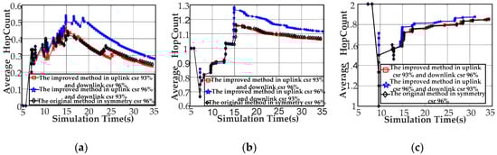
Figure 11.
Node simulation results for the average hop count. (a) Average hop count for node[0]; (b) average hop count for node[2]; and (c) average hop count for node[8].
Figure 12 mainly shows the statistic hop count histogram to stations (node[0], node[2], and node[8]) to illustrate the importance of the station in the network. We draw a conclusion that CCo (node[0]) is the zero hop station (root station); node[2] is the first hop station; and node[8] is the second hop station. Take node[2] as an example. We explain the statistic hop count results in different channel conditions, as shown in Figure 12b. Compared to the symmetric channel-based Q-learning featuring a success ratio of 96%, the proposed method performs approximately 21.3% above the statistic hop count maximum value under the traffic environment of uplink 96% success ratio and a 93% downlink success ratio. Compared to the Q-learning, we improve 13.6% at the statistic hop count by the proposed approach under the circumstances of uplink 93% success ratio and downlink 96% success ratio. Similar conclusions can be drawn in other stations.
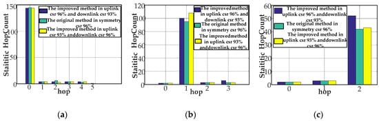
Figure 12.
Hop versus statistic hop count. (a) Hop versus statistic count for node[0]; (b) hop versus statistic count for node[2]; and (c) hop versus statistic count for node[8].
5.2. Network Performance Simulation
Our study simulates the saturation bandwidth utilization and access delay performance at a PHY transmission rate of 1 Mbps.
5.2.1. Network Saturation Performance Simulation
We investigated cases with 2, 5, 10, and 20 stations. The bandwidth utilization decreased as the bit error rate (BER) gradually increased. The bandwidth utilization for a BER greater than 0.0004 approached zero (Figure 13).
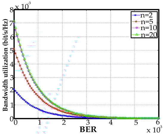
Figure 13.
Throughput versus BER.
Figure 14 depicts the relationship between the bandwidth utilization and the number of stations for a payload of 128 B. When , the bandwidth utilization decreased by 5.9% for a BER of 0.00005 compared to . When , the bandwidth utilization decreased by 9.6% at a BER of 0.00008 compared to The bandwidth utilization improved by 1.8% at and , relative to its utilization at and . The bandwidth utilization by the improved adaptive p-CSMA decreased by 3.5% and 1.8% at compared to the adaptive p-CSMA.
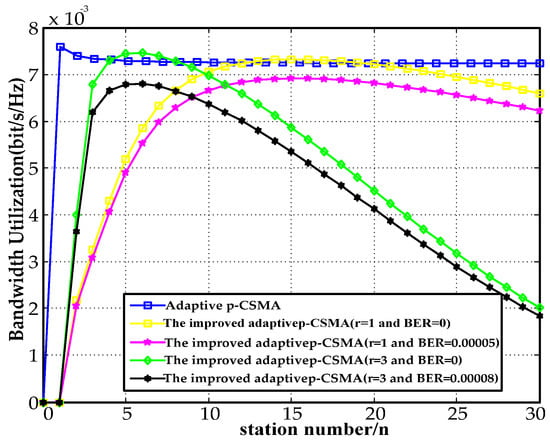
Figure 14.
128 B payload bandwidth utilization.
Figure 15 depicts the bandwidth utilization results for a payload of 512 B. At , the bandwidth utilization decreased by 34% at a BER of 0.0001 relative to a BER of 0. Similarly, when the BER was zero, the bandwidth utilization improved by 1.1% at relative to . The bandwidth utilization decreased by 19% between and The bandwidth utilization by the improved adaptive p-CSMA decreased by 1.9% and 1% for compared to the adaptive p-CSMA. The bandwidth utilization increased by 7% and 16.2% at compared to a payload of 128 B.
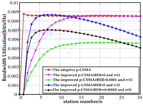
Figure 15.
512 B payload bandwidth utilization.
Figure 16 depicts the relationship between the access delays and the station numbers for 128 and 512 B payloads. The access delays for a payload of 128 B were increased by 9.4%, which was 2.57 times by the improved adaptive p-CSMA at relative to the adaptive p-CSMA. The delays for a payload of 512 B increased by 0.75% and 36.2% at Compared to the results for a payload of 128 B, the access delays were improved by 2.12% and 29.6% at .
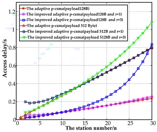
Figure 16.
Comparison of access delay.
5.2.2. Stations Numbers Estimation Simulation
Let us use 20 adjacent time slots as an example. Each time slot is 50 ms, and the channel states do not change for each time slot. The detailed parameters are as follows: assuming that the channel is initially idle, the Markov transition probability of the channel is , and the steady-state probability is . The channel state of the 20 adjacent time slots was calculated using the Markov chain model.
Matrix for stations 1 to 30 is calculated as follows:
Matrix A was obtained by calculation. The number of competitive stations for each station was estimated using the HMM. We performed simulations for 5, 10, 15, and 20 stations. The stations were peer-to-peer, and the number of competitive stations was estimated. We used a single station as an example to explain the results of the game between stations. The game mechanisms for the other stations were the same and not repeated herein.
The comparison results for the MAP algorithm and the proposed method were provided from the abovementioned parameters.
For asymmetric channels and noise interference in an LVPLC environment, the average bandwidth utilization of the time slots was relative to the results of the MAP algorithm. For 5, 10, 15, and 20 stations, the average bandwidth utilization in the time slots by the proposed method increased by 89.2% and 51.3% (Figure 17). The MAP algorithm only used the current time to estimate the number of stations. The results were not modified, and the accuracy was relatively low. The proposed method used the emission probabilities to estimate the number of stations. It produced more accurate information regarding competitive stations, guaranteeing network saturation performance at a cost of space and time complexity.
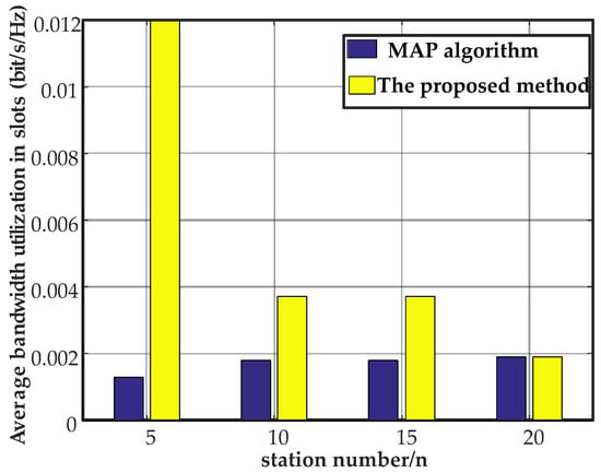
Figure 17.
Comparison of the two algorithms.
6. Conclusions
For asymmetric and error-prone channels, we herein proposed an improved adaptive p-persistent CSMA based on dynamic game to optimize the saturation performance of an improved LVPLC artificial cobweb in a typical home local area network scenario. The following results are obtained:
- (i)
- An improved Q-learning based hybrid CSMA/TDMA protocol was proposed to address the instability problem. The proposed method self-adaptively undertakes hop-by-hop learning to network under the variable channel conditions. Compared to the symmetrical channel, quantitative statistics on the average throughput, end to end delay, and hop count for stations under the asymmetrical constraint factor could be gathered when the system had completed the network functions.
- (ii)
- The bandwidth utilizations and access delays were improved by controlling the r values. The maximum bandwidth utilization improved by 1.7%, while the maximum access delays improved by a factor of 2.57, relative to the original model. The average bandwidth utilization of the time slots at maximum values improved by 89.2%, relative to the results of the MAP algorithm.
This proposed method is able to improve the network throughput, which will reduce the access delay and the collision probability of data packet in the home local area networks. In addition, the proposed method may also be applied in power distribution networks with automatic meter reading/advanced metering infrastructure, and vehicle-to-grid communications requirements. In future research, we plan to extend this work to a multi-network fusion and maintenance technology in the LVPLC.
Author Contributions
All the authors contributed to publish this paper. Ying Cui, Xiaosheng Liu, Jian Cao and Dianguo Xu mainly proposed the scheme of this paper. Ying Cui has done the writing, carried out the simulation and Xiaosheng Liu has checked the simulation results. Ying Cui, Xiaosheng Liu, Jian Cao and Dianguo Xu corrected and finalized the paper.
Acknowledgments
This work is supported by National Natural Science Foundation of China (No. 51677034) and the Key Program of Natural Science Foundation of Heilongjiang Province in China (ZD2018012).
Conflicts of Interest
The authors declare no conflicts of interest.
References
- Wang, K.; Hu, X.; Li, H.; Li, P.; Zeng, D.; Guo, S. A Survey on Energy Internet Communications for Sustainability. IEEE Trans. Sustain. Comput. 2017, 2, 231–254. [Google Scholar] [CrossRef]
- Yigit, M.; Gungor, V.C.; Tuna, G.; Rangoussi, M.; Fadel, E. Power line communication technologies for smart grid applications: A review of advances and challenges. Comput. Netw. 2014, 70, 366–383. [Google Scholar] [CrossRef]
- Masood, B.; Baig, S. Standardization and deployment scenario of next generation NB-PLC technologies. Renew. Sustain. Energy Rev. 2016, 65, 1033–1047. [Google Scholar] [CrossRef]
- Rahman, M.M.; Hong, C.S.; Lee, S.; Lee, J.; Razzaque, M.A.; Kim, J.H. Medium access control for power line communications: An overview of the IEEE 1901 and ITU-T G. hn standards. IEEE Commun. Mag. 2011, 49, 183–191. [Google Scholar] [CrossRef]
- Jian, L.; Qiang, S. The study on the performance of backoff algorithms in multihop power line communication networks. In Proceedings of the Third International Conference on Measuring Technology and Mechatronics Automation (ICMTMA), Shangshai, China, 6–7 January 2011; pp. 974–977. [Google Scholar]
- Chang, D.; Cho, K.; Choi, N.; Choi, Y. A probabilistic and opportunistic flooding algorithm in wireless sensor networks. Comput. Commun. 2012, 35, 500–506. [Google Scholar] [CrossRef]
- Hanashi, A.M.; Siddique, A.; Awan, I.; Woodward, M. Performance evaluation of dynamic probabilistic broadcasting for flooding in mobile ad hoc networks. Simul. Model. Pract. Theory 2009, 17, 364–375. [Google Scholar] [CrossRef]
- Li, F.Y.; Hafslund, A.; Hauge, M.; Engelstad, P.; Kure, Ø.; Spilling, P. Does Higher Datarate Perform Better in IEEE 802.11-based Multi-hop Ad Hoc Networks. J. Commun. Netw. 2007, 9, 282–295. [Google Scholar] [CrossRef]
- Ahmed, M.A.; Kang, Y.C.; Kim, Y.C. Communication Network Architectures for Smart-House with Renewable Energy Resources. Energies 2015, 8, 8716–8735. [Google Scholar] [CrossRef]
- Vlachou, C.; Banchs, A.; Salvador, P.; Herzen, J.; Thiran, P. Analysis and Enhancement of CSMA/CA with Deferral in Power-Line Communications. IEEE J. Sel. Areas Commun. 2016, 34, 1978–1991. [Google Scholar] [CrossRef]
- Zhang, L.; Liu, X.; Zhou, Y.; Xu, D. A novel routing algorithm for power line communication over a low-voltage distribution network in a smart grid. Energies 2013, 6, 1421–1438. [Google Scholar] [CrossRef]
- Liu, X.S.; Qi, J.J.; Song, Q.T.; Li, Y.; Xu, D.G. Method of constructing power line communication networks over low-voltage distribution networks based on ant colony optimization. Proc. CSEE 2008, 28, 71–76. [Google Scholar]
- González-Sotres, L.; Frías, P.; Mateo, C. Power line communication transfer function computation in real network configurations for performance analysis applications. IET Commun. 2017, 11, 897–904. [Google Scholar] [CrossRef]
- Kriminger, E.; Latchman, H. Markov chain model of HomePlug CSMA MAC for determining optimal fixed contention window size. In Proceedings of the IEEE International Symposium on Power Line Communications and Its Applications (ISPLC), Udine, Italy, 3–6 April 2011; pp. 399–404. [Google Scholar]
- Yoon, S.-G.; Yun, J.; Bahk, S. Adaptive contention window mechanism for enhancing throughput in homeplug AV networks. In Proceedings of the IEEE 5th Consumer Communications and Networking Conference (CCNC), Las Vegas, NV, USA, 10–12 January 2008; pp. 190–194. [Google Scholar]
- Vlachou, C.; Banchs, A.; Herzen, J.; Thiran, P. How CSMA/CA with Deferral Affects Performance and Dynamics in Power Line Communications. IEEE Trans. Netw. 2017, 25, 250–263. [Google Scholar] [CrossRef]
- Liu, D.; Xu, Y.; Shen, L.; Xu, Y. Self-organising multiuser matching in cellular networks: A score-based mutually beneficial approach. IET Commun. 2016, 10, 1928–1937. [Google Scholar] [CrossRef]
- Shi, Y.; Hou, Y.T. A distributed optimization algorithm for multi-hop cognitive radio networks. In Proceedings of the IEEE 27th Conference on Computer Communications (INFOCOM), Phoenix, AZ, USA, 13–18 April 2008; pp. 1292–1300. [Google Scholar]
- Chakraborty, S.; Dash, D.; Sanyal, D.K.; Chattopadhyay, S.; Chattopadhyay, M. Game-theoretic wireless CSMA MAC protocols: Measurements from an indoor testbed. In Proceedings of the IEEE Conference on Computer Communications Workshops (INFOCOM WKSHPS), San Francisco, CA, USA, 10–14 April 2016; pp. 1063–1064. [Google Scholar]
- Zhang, Y.; He, J. A proactive access control model based on stochastic game. In Proceedings of the 4th International Conference on Computer Science and Network Technology (ICCSNT), Harbin, China, 19–20 December 2015; pp. 1008–1011. [Google Scholar]
- Tonello, A.M.; Versolatto, F. Bottom-Up Statistical PLC Channel Modeling-Part I: Random Topology Model and Efficient Transfer Function Computation. IEEE Trans. Power Deliv. 2011, 26, 891–898. [Google Scholar] [CrossRef]
- Ahmed, M.O.; Lampe, L. Power Line Communications for Low-Voltage Power Grid Tomography. IEEE Trans. Commun. 2013, 61, 5163–5175. [Google Scholar] [CrossRef]
- Zhang, L.; Liu, X.S.; Pang, J.W.; Xu, D.G.; Leung, V.C.M. Reliability and Survivability Analysis of Artificial Cobweb Network Model Used in the Low-Voltage Power-Line Communication System. IEEE Trans. Power Deliv. 2016, 31, 1980–1988. [Google Scholar] [CrossRef]
- Wu, C.; Ohzahata, S.; Kato, T. Flexible, portable, and practicable solution for routing in VANETs: A fuzzy constraint Q-learning approach. IEEE Trans. Veh. Technol. 2013, 62, 4251–4263. [Google Scholar] [CrossRef]
- Vázquez-Rodas, A.; Luis, J. A centrality-based topology control protocol for wireless mesh networks. Ad Hoc Netw. 2015, 24, 34–54. [Google Scholar] [CrossRef]


© 2018 by the authors. Licensee MDPI, Basel, Switzerland. This article is an open access article distributed under the terms and conditions of the Creative Commons Attribution (CC BY) license (http://creativecommons.org/licenses/by/4.0/).