Abstract
This paper presents the scheduling dispatch of a microgrid (MG), while considering renewable energy, battery storage systems, and time-of-use price. For the risk evaluation of an MG, the Value-at-Risk (VAR) is calculated by using the Historical Simulation Method (HSM). By considering the various confidence levels of the VAR, a scheduling dispatch model of the MG is formulated to achieve a reasonable trade-off between the risk and cost. An Improved Bee Swarm Optimization (IBSO) is proposed to solve the scheduling dispatch model of the MG. In the IBSO procedure, the Sin-wave Weight Factor (SWF) and Forward-Backward Control Factor (FBCF) are embedded in the bee swarm of the BSO to improve the movement behaviors of each bee, specifically, its search efficiency and accuracy. The effectiveness of the IBSO is demonstrated via a real MG case and the results are compared with other methods. In either a grid-connected scenario or a stand-alone scenario, an optimal scheduling dispatch of MGs is carried out, herein, at various confidence levels of risk. The simulation results provide more information for handling uncertain environments when analyzing the VAR of MGs.
1. Introduction
Distributed Generators (DGs) have been extensively utilized during the last decade. DGs offer reliable, efficient, and economic energy, and will be an important alternative energy production option in the near future [1]. They can be constructed in urban areas and produce power with islanding energy to sell back to utility companies. A typical microgrid (MG) portfolio of resources may include photovoltaics (PV), small wind turbines (WT), fuel cells, and micro-turbines, which can all be connected to the grid. MGs can operate in either a grid-connected mode or stand-alone mode [2], and usually require a scheduling dispatch strategy to ensure stable operation. Since MGs can decrease electricity cost and increase energy efficiency, their employment in the electricity market is still expanding [3,4]. For the MGs’ dispatch, more experience is needed regarding the efficient operation for realizing greater energy saving.
MGs are an important research field and several algorithms have been presented in energy management to improve energy efficiency and reduce power losses [5,6,7,8,9,10]. Due to some DGs, such as WTs and PVs, randomly generating output, they will not meet the load profile, making it difficult to produce accurate day-ahead schedules for MGs. Therefore, energy storage systems (EES) play an important role in enabling those operations to enjoy a more flexible and reliable management of energy [11]. EES can save energy during low price periods and sell it during high price periods, thereby, helping MGs operate more efficiently and economically. EES scheduling is used to reduce the peak load management by using evolutionary combinatorial optimization [12]. Ghaithi et al. investigated the technical and economic viability of a hybrid EES integrated within an existing diesel off-grid/isolated system. The results showed that the hybrid EES is the most economically feasible option as it provides the lowest operating cost [13]. References [14,15] analyzed the economic feasibility of integrating an EES. They also proved that EES with different capacities can improve power quality. However, there is a certain amount of unprecedented volatility and risk in MGs due to increasing stochastic generations of DGs being introduced. The scheduling dispatch in MGs is, therefore, more complicated and challenging.
An optimal scheduling dispatch of MGs is performed to minimize the operating cost. The biggest challenge comes from the intermittent nature of renewable DGs, namely the unpredictable nature and stochastic generation. By appropriate daily scheduling of units in MGs and minimizing the risks of dependency on the grid, MG owners and investors can schedule the renewable DGs to maximize their profits, while ensuring higher levels of energy security and reliability [16]. Since the profit may be at risk due to uncertain renewable DGs in scenario-based stochastic programs, risk assessment, which is crucial in optimization under uncertainty, can provide valuable information to decision makers. Comprehensive risk assessments can help provide a full distribution of profitability outcomes before making a decision. Value at Risk (VAR), a viable measurement for risk analysis, is used by financial institutions to measure the minimum loss expected in any given portfolio within an assigned period [17,18]. To limit the risk, risk assessment is proposed, in the objective function, using the VAR method.
Several approaches have been reported in the research literature on smart grids, in relation to risk management, applicable within the smart grid system. Ref. [19] presented a novel energy-management method for a microgrid that includes renewable DGs. In order to address various uncertainties, a risk-constrained scenario-based stochastic programming framework was proposed using conditional VAR. Ref. [20] presented a comparative study on the integration of renewable generation uncertainties into stochastic security and constrained unit commitment, considering reserve and risk. Ref. [21] explored the impact of uncertainty and risk aversion on unit commitment decisions in isolated systems with high renewable penetration. The proposed optimal solutions can provide valuable information to help d ecision makers seeking a trade-off between risk mitigation and overall costs. Ref. [22] presented a stochastic Unit Commitment (UC) model with high renewable penetration for the efficient management of uncertainty. A minimum conditional value at risk (CVAR) term was included in the UC model to evaluate the risk. As wind power generation penetration increases in smart grids, more innovative and sophisticated approaches to system operation are being adopted due to the intermittency and unpredictability of wind power generation [23,24]. Ref. [25] addressed the risk and UC decisions in scenarios involving wind power uncertainty. Ref. [26] proposed a Cost-CVAR model to determine an optimal spinning reserve for a wind power penetration system. Although some works have considered the uncertainties of renewable energy, the uncertainties of WTs and PVs have seldom been considered simultaneously. In addition, the scheduling dispatch of DGs in the MG is a particular issue in that it can be formulated as a non-linear and mixed-integer problem. Some techniques, such as Particle Swarm Optimisation (PSO), the Fuzzy Advanced Quantum Evolutionary Method (FAQA), the Chaotic Quantum Genetic Algorithm (CQGA), and the Artificial Bee Colony (ABC), etc., have been proposed to solve this problem and have shown their effectiveness [27,28,29,30,31]. The common drawback of these techniques is the lack of guarantee that the optimal solutions will always be located in a local optimum. To overcome the local optimum, an Improved Bee Swarm Optimisation (IBSO) is proposed in this paper.
This paper presents a scheduling dispatch of an MG by considering the uncertainties of WTs and PVs. Based on the historical data, the Value-at-Risk (VAR) of the penetrated WTs/PVs was simulated using the Historical Simulation Method (HSM) [32]. Due to the recent data being more indicative of future conditions than the forward data, the Exponentially Weighted Moving Average Approach (EWMAA) was embedded in the HSM to improve this shortcoming. By considering the VAR at various confidence levels, a scheduling dispatch model of an MG in a grid-connected or stand-alone scenario was formulated. An IBSO is proposed to solve the above-mentioned problem. In the IBSO procedure, the Sin-wave Weight Factor (SWF) and Forward-Backward Control Factor (FBCF) are embedded in the Bee Swarm Optimisation (BSO) to find a better solution. Combining the fundamentals of Value-at-Risk (VAR) analysis and the scheduling dispatch of an MG, users can capture the uncertainties of MGs for valuing the risk at an assigned confidence level. The simulation results can provide more information for handling energy uncertainty, in order to obtain the maximal profit and improve competitiveness.
2. Uncertainty Representation with Renewable Generation
2.1. VAR Calculation
VAR is an estimate of loss resulting from environmental fluctuations for a given probability of occurrence. The given probability is called the confidence level, which represents the degree of the VAR. The common value of a confidence level is 95%, which means that 95% of the time the participants’ loss will be less than the VAR, while 5% of the time the loss will be more than the VAR, as shown in Figure 1. The purpose of this paper is to propose a novel method for evaluating widespread WTs/PVs under various scenarios. Based on historical data, the VAR of the WTs/PVs’ penetration is simulated using the HSM. Due to the recent data being more indicative of future conditions than the forward data, the Exponentially Weighted Moving Average Approach (EWMAA) was used to improve the shortcomings. The formulation of the EWMAA is expressed in Equation (1):
where is the weight factor for the historical data, N is the total number of the historical data, is the decay factor, and is the current time.
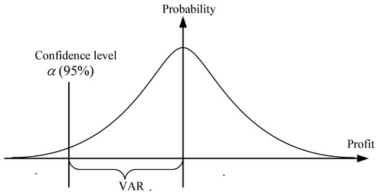
Figure 1.
Diagram of the Value at Risk (VAR) calculation.
The procedure for the VAR calculation for the WTs/PVs is described in the following steps.
- Step 1.
- Retrieve the historical data:The wind speed and global irradiance for the WTs and PVs were retrieved from the historical data.
- Step 2.
- Calculate the rate of change for the wind speed/global irradiance:: The wind speed or global irradiance at time t.
- Step 3.
- Sort the rate of change from small to large.
- Step 4.
- Calculate the critical value of the rate of change in a confidence value, α%
- Step 5.
- Multiply the critical value of the rate of change by the wind speed/global irradiance value to derive the VAR (
- Step 6.
- Combine the EWMAA and decay factor, so that the VAR of the following data is calculated. When all historical data are completed, the operation stops. If the pre-set target is not yet attained, go back to Step (1) and repeat the operation. In this paper, there were 720 items of historical data.
2.2. The Power Output of the WT Uncertainty
The WT output between the wind speed and mechanical power extracted can be explained as follows [33]:
, which is the performance coefficient of wind power, is assigned as follows:
The ON/OFF status of the WT is described as follows:
By considering the VAR of the wind speed, the VAR of the WT output can be expressed, as in Equation (6):
: Power output from the wind (kw) at time t
: Air density (kg/m3)
Area covered by the rotor (m2)
: Wind speed (m/s) at time, t
: VAR of the wind speed (m/s) at time, t
: Tip speed ratio
: Pitch angle of the rotor blades (deg.)
: Start wind speed (m/s)
: Rated wind speed (m/s)
: Stop wind speed (m/s)
2.3. The Power Output of the PV Uncertainty
The power output of PV can be calculated as follows [34]:
where, represents PV output power at time t, is the global radiation (w/m2) at time t, is the area of the PV array (m2), and is the efficiency of PV.
By considering the VAR of the global radiation, the VAR of the PV output can be expressed as Equation (8):
: VAR of the global radiation (w/m2) at time, t.
2.4. The Fuel Cost of Diesel Oil Unit
The diesel oil unit is considered as a DG, which generates a constant power output. The fuel cost of the diesel oil unit is considered as a quadratic model, which is expressed as Equation (9):
is the fuel cost of unit, , at time, . are the coefficients of the production cost of unit, , and is the power output of a committed unit, i, at time, .
2.5. Model for Battery Storage
The power output of a battery can be calculated as the difference between the stored energies of two consecutive stages. Energy stored in the battery device is expressed as follows [35]:
- If the battery is charging:
- If the battery is discharging:where and are the charging efficiency and the discharging efficiency, respectively. is the electrical power of the battery output at the hour. is the aggregated capacity of the batteries at hour. is the rated maximum storage energy. / is the maximum portion of the rated capacity that can be added to/withdrawn from storage in an hour. is the scheduling hour. In this paper, was equal to 1 h.
3. Mathematical Formulation
The scheduling dispatch of the MGs was based on stochastic mixed non-linear programming. The objective function can be formulated as Equation (14):
H: Scheduling time
N: Total number of micro gas turbines
/: Purchased from/sold to electricity price at time, t
/: Electricity purchased/sold of the utility at time t ()
The following constraints are also defined:
- (a)
- Load balance:
- (b)
- Unit power generation limitation:
- (c)
- Ramp up rate:
- (d)
- Ramp down rate:
- (e)
- Electricity bought/sold of utility:
: System demand at time t
/: Maximum/minimum generation limits of unit i
/: Ramp up/down limit of unit i
: Active power bought/sold of the utility at time t
: Maximum active power bought/sold of the utility at time t
4. Methodology
This paper proposes an Improved Bee Swarm Optimization (IBSO) to solve the scheduling dispatch of MGs under uncertainty and with renewable generation. BSO, which simulates the food foraging behavior of bees, was developed by [36]. In BSO, a hard restriction exists on the flying pattern of the bees. Because the information exchange of a bee swarm is imperfect, it may cause premature convergence. IBSO is proposed to further improve BSO. IBSO is developed as follows.
4.1. Initial Solutions
The initial populations were filled with a number of food sources (NFS) randomly generated in a limited area. The random positions of the food sources were generated by:
where is the food scout of the solution vector, . and represent the lower and upper boundaries of the solution vector, , and is a uniformly distributed random number in the range of (0,1).
4.2. Employed Bee Phase
In IBSO, most the employed bees fly in consideration of the social and cognitive information recieved by the swarm. Each bee knows its current optimal position , which is analogous to the personal experiences of each particle. Each bee also knows the current global optimal position ( among all the bees in the population. IBSO can derive several solutions concurrently, while particles have a cooperative relationship for sharing messages. In other words, it tries to achieve compatibility between the local search and the global search. At this stage, each employed bee makes a change in the position of the food sources, thus, generating a new food source in the neighborhood of its present position as follows:
where is a random number between 0 and 1, is a randomly chosen index, and , , and are the weight factor. is the concept of the interference factor, is the current iteration, and is the number of employed bees.
4.2.1. Sin-Wave Weight Factor (SWF)
In this paper, and , were improved as the Sin-wave Weight Factor (SWF), which uses the resonance principle to produce the effect of an interlaced search, and effectively searches for a better result. With the integrational non-linear sine wave and time-varying iteration, the formulation of and can be defined as follows:
where,
is a sin-wave function, is the maximal iteration, and is a ripple constant value (0.11). Due to the different ripple values having different resonance curves, H was used to extend the feasible search area to ensure the best solution. Figure 2 shows the influenced characteristics of a ripple wave during 300 iterations, when H is equal to 0.1. With increasing numbers of iterations, a wide range of the local search is guaranteed to search the global optimum due to the larger ripple factor.
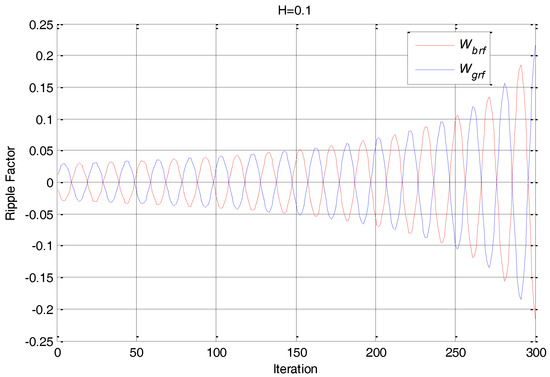
Figure 2.
Influenced characteristics of a ripple wave at the ripple constant value, H = 0.1.
4.2.2. Forward-Backward Control Factor (FBCF)
This paper introduces the Forward-Backward Control Factor (FBCF) to enhance the global search capability of IBSO. This factor can fly over some parts of the search space and may include profitable information by the bee swarm. The increasing diversity of a bee swarm can avoid premature convergence. To enlarge the search area to include areas that might have been neglected, the concept of the interference factor, , was introduced in Equation (24):
where is the control factor and the initial setting of is 0.5. When the randomly generated is larger than the predefined , a reverse search will take place. is the interference factor. The values used by bee swarms were recorded and adjusted according to the fitness value in each iteration. Figure 3 shows the initial relationship of FBCF; in this paper it was set to and . If was produced, let to increase the probability of the forward foraging direction for the bees, as shown in Figure 4. Conversely, if in the current iteration, it was generated at , the probability of foraging in the backward region should be increased, as shown in Figure 5.

Figure 3.
Probability map of control factor for the control factor, CV = 0.5.
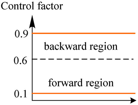
Figure 4.
Variation of probability of the interference factor, .
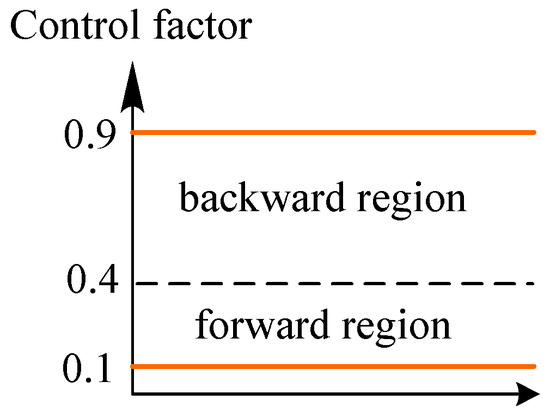
Figure 5.
Variation of probability of .
4.3. Onlooker Bees
The onlooker bees in the improved bee swarm algorithm followed the employed bees to obtain nectar information without joining the group of employed bees. The flying path of the onlooker bees following the employed bees was modified by using the probabilistic selection method, as shown in Equation (25). In the working mode of the onlooker bees, the repulsive force was also included to enlarge the search area, as shown in Equation (26):
where is the probability of better food source and is the best food source, is the employed bee population, and is the onlooker bee population.
4.4. Scout Bees
In IBSO, the model of the scout bees is not a baseless random search. The working model of the scout bees adopts the average value of the global optimum solution and all swarm locations. After comparison, the new location of scout bees was generated by Equation (27):
where the variable is the number of scout bees and is the average of all variable solutions in the iteration.
4.5. Stop Condition
The terminating condition is the maximal number of iterations. If the pre-set target is not yet attained, Step (2) was returned to and the operation was repeated. This paper set the stop condition at 200 generations.
5. Simulation Results
The proposed algorithm was tested for the Penghu MG, as shown in Figure 6. The configuration of the MG system consisted of 12 diesel oil units, 2 WT fields, 2 PV fields, and one battery storage. The system was exchanged with the TPC utility from the Tai-pen power line. The associated data for Penghu MG are listed in Table 1. The data, including the wind speed and global radiation in the different scenarios, was collected, and the time horizon chosen is one day divided into 24 hourly periods, as shown in Figure 7 and Figure 8. Figure 7 shows the wind speed scenarios of the Chongtun/Huhs WT from 2 December 2016 to 20 December 2016. Figure 8 shows the global radiation scenarios of the Jianshan/Cimei PV from 2 December 2016 to 20 December 2016.
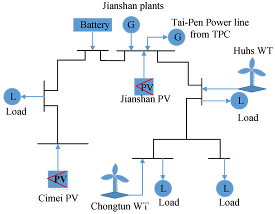
Figure 6.
Construction of Penghu microgrid (MG).

Table 1.
Associated data of Penghu MG.
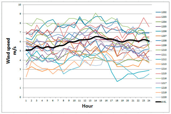
Figure 7.
Wind speed scenarios of Chongtun/Huhs small wind turbines (WT).
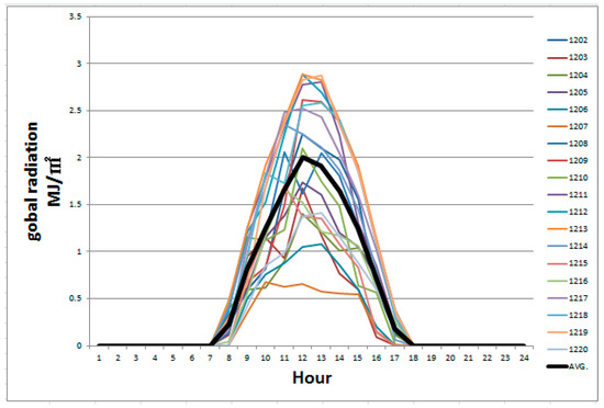
Figure 8.
Global radiation scenarios of Jianshan/Cimei photovoltaics (PVs).
5.1. VAR of WTs and PVs’ Generation in Different Scenarios
A VAR calculation for different risk levels using the HSM is presented in this paper. From the historical data, as shown in Figure 7 and Figure 8, the VAR of the WTs and PVs’ generation for the different risk levels was calculated in Figure 9 and Figure 10. These figures show the ability of the WT/PV generation to operate in the day-ahead market, taking into account the desired risk level.
Figure 9.
Power generation of WTs for the different risk levels.
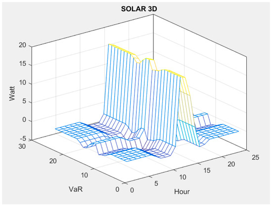
Figure 10.
Power generation of PVs for the different risk levels.
5.2. Results in the Grid-Connected Scenario
Figure 11 shows the generation supply scheme and dispatch cost at the 95% confidence level. The total generation supplied in one day was 98.29%, 1.65%, and 0.06% for the utility units, the WT unit and PV unit, respectively. Due to the electricity purchased from the utility being cheaper than the production cost of the Jianshan plants, the power from the utility units was used to meet the biggest load demand. The generation of the Jianshan plants was zero during all periods. During the scheduling duration, the load demand needs be satisfied, while considering the charging/discharging scheduling of the battery. With cooperation of the battery and other DGs, the cost was about NT$3,668,568 through the control sequence determined by the optimizing dispatch.
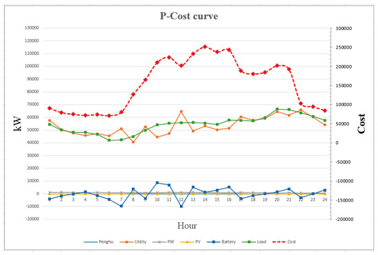
Figure 11.
Generation supply scheme and dispatch cost at the 95% confidence level.
Table 2 shows the VAR at the various confidence levels (α = 95%, α = 90%, and α = 85%). The VAR in the whole scheduling period corresponding to 95%, 90%, and 85% was NT$3,668,568, NT$3,654,917, and NT$3,622,124, respectively. According to Table 2, a higher confidence level led to lower risk, which was a higher VAR. VAR corresponds to a percentile of the portfolio cost distribution and can be expressed as a potential loss from the expected value at a period. MG can seriously evaluate its asset dependency at various VARs.
Table 2.
VAR at the various confidence levels.
5.3. Results in the Stand-Alone Scenario
Figure 12 shows the generation supply scheme and dispatch cost at the 95% confidence level. Due to the MG being operated in a stand-alone scenario, the generation supply of the utility is zero in one day. The power from the Jianshan plants is used to meet the biggest load demand. With the use of the battery and other DGs, the operating cost is about NT$6,815,360 through the control sequence determined by the optimizing dispatch.
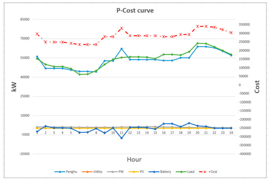
Figure 12.
Generation supply scheme in the stand-alone scenario.
Table 3 shows the VAR at the various confidence levels (α = 95%, α = 90%, α = 85%). The VAR in the whole scheduling period corresponding to 95%, 90%, and 85% is NT$6,815,360, NT$6,807,893 and NT$6,797,139, respectively. According to Table 2, a higher confidence level also led to lower risk, which was a higher VAR. VAR corresponds to a percentile of the portfolio cost distribution and can be expressed as a potential loss from the expected value at a period. MG can seriously evaluate its asset dependency on various VARs.
Table 3.
VAR at the various confidence levels.
5.4. Convergence Test
Table 4 and Table 5 list the comparisons of the algorithms of EP, GA, PSO, BSO, and IBSO in the grid-connected scenario and stand-alone scenario, respectively. The tests were carried out on an Intel Core i5-3470s 2.9Hz CPU (Intel, Santa Clara, CA, USA), with 8 GB DRAM. Each algorithm was executed with 100 trials, with the same initial parents. It can be seen that IBSO improved searching performance and had the best probability of guaranteeing a global optimum. From Table 4 and Table 5, with IBSO’s better accuracy, the number of trials reaching the optimum was better than EP, GA, PSO, and BSO. Although the average executed time was also much less than GA and a little more than EP, PSO, and BSO, the average number of generations to converge was only 153. The practical executed time of IBSO was less than that of the other algorithms. Figure 13 and Figure 14 illustrate the convergence characteristics of EP, GA, PSO, BSO, and IBSO in the grid-connected scenario and stand-alone scenario. They also show that the capacity of IBSO reflects the ability to explore a more likely global optimum.
Table 4.
Tests for the EP, GA, PSO, BSO, and IBSO algorithms in the grid-connected scenario.
Table 5.
Tests for the EP, GA, PSO, BSO, and IBSO algorithms in the stand-alone scenario.
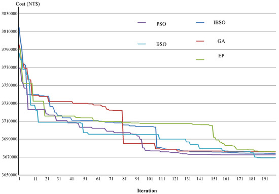
Figure 13.
Convergence characteristics of the EP, GA, PSO, BSO, and IBSO algorithms in the grid-connected scenario.
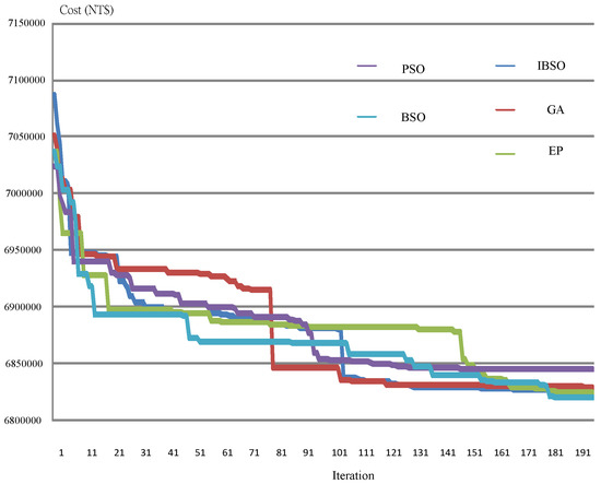
Figure 14.
Convergence characteristics of the EP, GA, PSO, BSO, and IBSO algorithms in the stand-alone scenario.
6. Conclusions
Based on renewable energy generation, the VAR is calculated at an assigned confidence level to quantify the risk created by renewable energy uncertainty, while minimizing the overall system cost. IBSO integrates the Sin-wave Weight Factor (SWF) and Forward-Backward Control Factor (FBCF) to provide a better global exploration capability and it can improve the quality of results in the optimization problem. Two scenarios, a grid-connected scenario and a stand-alone scenario, were evaluated at different confidence levels to minimize the operational costs of the MGs. In either scenario, optimal scheduling in renewable energy uncertainty was carried out by operating the renewable energy and battery storage systems. The effectiveness of the proposed algorithm in solving scheduling dispatching was tested on a real MG system to explore the impact of uncertainty and risk aversion on dispatch decisions with high renewable penetration. The results can help decision-makers to handle valuable information on the trade-off between risk assessment and operating cost. The proposed algorithm can also be applied for further application to many other mixed-integer combinational optimization problems in power system planning and operation.
Author Contributions
W.-M.L. designed the algorithm and handled the project as the first author. C.-Y.Y. performed the experiments and conducted simulations. M.-T.T. assisted the project and prepared the manuscript as the corresponding author. C.-S.T. contributed materials tools. All the authors discussed the simulation results and approved the publication.
Acknowledgments
The authors would like to acknowledge the financial support for this work by the Ministry of Science and Technology of the R.O.C. under contract number MOST 106-2221-E-230-008, which is gratefully appreciated.
Conflicts of Interest
The authors declare no conflict of interest.
References
- Huang, J.; Jiang, C.; Xu, R. A review on distributed energy resources and Microgrid. Renew. Sustain. Energy Rev. 2008, 12, 2472–2483. [Google Scholar] [CrossRef]
- Katiraei, F.; Iravani, R.; Hatziargyriou, N.; Dimeas, A. Microgrids management. IEEE Power Energy Manag. 2008, 6, 54–65. [Google Scholar] [CrossRef]
- Faber, I.; Lane, W.; Pak, W.; Prakel, M.; Rocha, C.; Farr, J.V. Micro-energy markets: The role of a consumer preference pricing strategy on microgrid energy investment. Energy 2014, 74, 567–575. [Google Scholar] [CrossRef]
- Hopkins, M.D.; Pahwa, A.; Easton, T. Intelligent Dispatch for Distributed Renewable Resources. IEEE Trans. Smart Grid 2012, 3, 1047–1054. [Google Scholar] [CrossRef]
- Zhao, B.; Dong, X.; Luan, W.; Bornemann, X. Short-term operation scheduling in renewable-powered microgrids: A duality-based approach. IEEE Trans. Sustain. Energy 2014, 5, 209–217. [Google Scholar] [CrossRef]
- Jiang, Q.; Xue, M.; Geng, G. Energy management of microgrid in grid-connected and stand-alone modes. IEEE Trans. Power Syst. 2013, 28, 3380–3389. [Google Scholar] [CrossRef]
- Barelli, L.; Bidini, G.; Bonucci, F. Micro-grid operation analysis for cost-effective battery energy storage and RES plants integration. Energy 2016, 113, 831–844. [Google Scholar] [CrossRef]
- Gabbar, H.A.; Abdelsalam, A.A. Microgrid energy management in grid-connected and islanding modes based on SVC. Energy Convers. Manag. 2014, 86, 964–972. [Google Scholar] [CrossRef]
- Juan, M.; Lujano, R.; Dufo-López, R.; José, L.; Eduardo, M.G. Operating conditions of lead-acid batteries in the optimization of hybrid energy systems and microgrids. Appl. Energy 2016, 179, 590–600. [Google Scholar]
- Zhong, H.; Xia, Q.; Xia, Y.; Kang, C.; Xie, L. Integrated dispatch of generation and load: A pathway towards smart grids. Electr. Power Syst. Res. 2015, 120, 206–213. [Google Scholar] [CrossRef]
- Rémy, R.M.; Bruno, S.; Xavier, R.; Christophe, T. Optimal power dispatching strategies in smart-microgrids with storage. Renew. Sustain. Energy Rev. 2014, 40, 649–658. [Google Scholar]
- Agamah, S.U.; Ekonomou, L. Energy storage system scheduling for peak demand reduction using evolutionary combinatorial optimization. Sustain. Energy Technol. Assess. 2017, 23, 73–82. [Google Scholar]
- Al Ghaithi, H.M.; Fotis, G.P.; Vita, V. Techno-economic assessment of hybrid energy off-grid system—A case study for Masirah island in Oman. Int. J. Power Energy Res. 2017, 1, 103–116. [Google Scholar] [CrossRef]
- Nieto, A.; Vita, V.; Ekonomou, L.; Mastorakis, N.E. Economic analysis of energy storage system integration with a grid connected intermittent power plant, for power quality purposes. WSEAS Trans. Power Syst. 2016, 11, 65–71. [Google Scholar]
- Nieto, A.; Vita, V.; Maris, T.I. Power quality improvement in power grids with the integration of energy storage systems. Int. J. Eng. Res. Technol. 2016, 5, 438–443. [Google Scholar]
- El-Hendawi, M.; Gabbar, H.A.; El-Saady, G.; Ibrahim, E.A. Control and EMS of a Grid-Connected Microgrid with Economical Analysis. Energies 2018, 11, 129. [Google Scholar] [CrossRef]
- Zhang, N. A convex model of risk-based unit commitment for day-ahead market clearing considering wind power uncertainty. IEEE Trans. Power Syst. 2015, 30, 1582–1592. [Google Scholar] [CrossRef]
- Alexander, C. Risk Management and Analysis—Volume 1 Measuring and Modeling Financial Risk; John Wiley & Sons Ltd.: Chichester, UK, 1998. [Google Scholar]
- Ji, L.; Huang, G.; Xie, Y.; Zhou, Y.; Zho, J. Robust cost-risk tradeoff for day-ahead schedule optimization in residential microgrid system under worst-case conditional value-at-risk consideration. Energy 2018, 153, 324–337. [Google Scholar] [CrossRef]
- Shen, J.; Jiang, C.; Liu, Y.; Wang, X. A microgrid energy management system and risk management under an electricity market environment. IEEE Acess 2016, 3, 2349–2356. [Google Scholar] [CrossRef]
- Quan, H.; Srinivasan, D.; Khosravi, A. Integration of renewable generation uncertainties into stochastic unit commitment considering reserve and risk: A comparative study. Energy 2016, 103, 735–745. [Google Scholar] [CrossRef]
- Asensio, M.; Contreras, J. Stochastic unit commitment in isolated systems with renewable penetration under cavr assessment. IEEE Trans. Smart Grid 2016, 7, 1356–1367. [Google Scholar] [CrossRef]
- Wang, C.; Liu, F.; Wang, J.; Wei, W.; Mei, S. Risk-based admissibility assessment of wind generation integrated into a bulk power system. IEEE Trans. Sustain. Energy 2016, 7, 325–336. [Google Scholar] [CrossRef]
- Pousinho, H.M.I.; Mendes, V.M.F.; Catalao, J.P.S. A risk-averse optimization model for trading wind energy in a market environment under uncertainty. Energy 2011, 36, 4935–4942. [Google Scholar] [CrossRef]
- Pinto, M.S.S.; Miranda, V.; Saavedra, O.R. Risk and unit commitment decisions in scenarios of wind power uncertainty. Renew. Energy 2016, 97, 550–558. [Google Scholar] [CrossRef]
- Wu, J.; Zhang, B.; Deng, W.; Zhang, K. Application of cost-cvar model in determining optimal spinning reserve for wind power penetrated system. Int. J. Electr. Power Energy Syst. 2015, 66, 110–115. [Google Scholar] [CrossRef]
- Moghaddam, A.A.; Seifi, A.; Niknam, T. Multi-operation management of a typical micro-grids using Particle Swarm Optimization: A comparative study. Renew. Sustain. Energy Rev. 2012, 16, 1268–1281. [Google Scholar] [CrossRef]
- Chakraborty, S.; Ito, T.; Senjyu, T.; Saber, A.Y. Intelligent Economic Operation of Smart-Grid Facilitating Fuzzy Advanced Quantum Evolutionary Method. IEEE Trans. Sustain. Energy 2013, 4, 905–916. [Google Scholar] [CrossRef]
- Liao, G.C. Solve environmental economic dispatch of Smart MicroGrid containing distributed generation system—Using chaotic quantum genetic algorithm. Int. J. Electr. Power Energy Syst. 2012, 43, 779–787. [Google Scholar] [CrossRef]
- Firouzi, B.B.; Farjah, E.; Abarghooee, R.A. An efficient scenario-based and fuzzy self-adaptive learning particle swarm optimization approach for dynamic economic emission dispatch considering load and wind power uncertainties. Energy 2013, 50, 232–244. [Google Scholar] [CrossRef]
- Marzband, M.; Azarinejadian, F.; Savaghebi, M.; Guerrero, J.M. An optimal energy management system for islanded microgrids based on multiperiod artificial bee colony combined with markov chain. IEEE Syst. J. 2015, 99, 1–11. [Google Scholar] [CrossRef]
- Marrison, C. Fundamentals of Risk Measurement; McGraw-Hill Companies, Inc.: New York, NY, USA, 2002. [Google Scholar]
- Slootweg, J.G.; Haan, S.W.H.; Polinder, H.; Kling, W.L. General model for representing variable speed wind turbines in power system dynamics simulations. IEEE Trans. Power Syst. 2003, 18, 144–151. [Google Scholar] [CrossRef]
- Wang, J.; Li, X.; Yang, H.; Kong, S. Design and Realization of Microgrid Composing of Photovoltaic and Energy Storage System. Energy Procedia 2011, 12, 1008–1014. [Google Scholar] [CrossRef]
- Chen, C.; Duan, S.; Cai, T.; Liu, B.; Hu, G. Smart energy management system for optimal microgrid economic operation. IET Renew. Power Gener. 2011, 6, 258–267. [Google Scholar] [CrossRef]
- Karaboga, D.; Akay, B. A comparative study of artificial bee colony algorithm. J. Appl. Math. Comput. 2009, 2014, 108–132. [Google Scholar] [CrossRef]


© 2018 by the authors. Licensee MDPI, Basel, Switzerland. This article is an open access article distributed under the terms and conditions of the Creative Commons Attribution (CC BY) license (http://creativecommons.org/licenses/by/4.0/).