1. Introduction
A two-phase closed thermosyphon, like a wicked heat pipe, transmits heat by the evaporation and condensation of a working fluid that is circulating in a sealed container. However, the thermosyphon relies on the force of gravity to return the working fluid from a condenser to an evaporator rather than relying on the capillary forces produced by the wick in the wicked heat pipe [
1]. As a kind of high-efficiency heat transfer component, a thermosyphon, whose internal complex heat and mass transfer is the focus of this research about the heat transfer mechanism of a heat pipe, has already been widely used in the field of heat exchange. Thermosyphon technology is playing an important role in many industrial applications, particularly in the heat transfer of heat exchangers and in energy savings in applications. For the advantages of its light weight, wide operating temperature range, compact structure, flexibility, high capacity of heat transfer, and great isothermal performance, the thermosyphon has been widely used in many cooling fields that contain electronic components and products [
2,
3,
4].
A thermosyphon consists of a condenser, an adiabatic section, and an evaporator section. The evaporator section is heated by a hot source, and the condenser section is cooled by a cold source. The adiabatic section placed between the condenser and evaporator sections is surrounded with thermal insulation layers. Heat is absorbed by the evaporator section with a liquid pool, which is situated at the bottom of the thermosyphon, following which liquid that absorbs the latent heat of evaporation is turned into vapor. Afterwards, vapor rises up to the condenser section at the top of the thermosyphon, where it is condensed and gives up latent heat. The condensed working fluid, which forms a liquid film along the walls, moves back to the evaporator under gravity.
A great variety of experiments have been done to understand the thermal characteristics of the thermosyphon [
5,
6,
7,
8,
9,
10,
11], although with an unknown internal heat and mass transfer mechanism. Annamalai and Ramalingam [
12] built a model for a wicked heat pipe by using ANSYS CFX and performing an experimental study. They assumed that the section inside the heat pipe was filled by the vapor phase, and the liquid phase only occurred in the wick section. The wall temperature of the condenser and evaporator and the vapor temperature were compared. Legierski et al. [
13] provided a model for simulating the temperature along the heat pipe walls at different moments and the vapor velocity inside the heat pipe. They considered the heat pipe as an open system, wherein the evaporator was treated as the inlet of mass flow and the condenser was treated as the outlet. The start-up time of the heat pipe was 20~30 s, and the evaporation coefficient of water was
. The range of effective thermal conductivity was also provided.
De Schepper et al. [
14] employed the user-defined function (UDF) and volume of fluid (VOF) techniques to calculate the phase-change of a hydrocarbon feedstock. They proposed that UDFs were specified as source terms, which were used to simulate heating and boiling in the convection section of a steam cracker. Lin et al. [
15] carried out a computational fluid dynamics (CFD) analysis of miniature oscillating heat pipes using VOF and mixture methods. Alizadehdakhel et al. [
16] performed an experimental study under different operating conditions in a thermosyphon. They also created a CFD model to compare the predicted temperature profile with experimental results that employed the VOF model.
Fadhl et al. [
17] carried out an experimental study and CFD analysis of a two-phase closed thermosyphon using the VOF technique. The experimental investigation was performed with the input heat powers of 100.41, 172.87, 225.25, 275.6, 299.52, and 376.14 W. The temperature profile predicted by CFD was consistent with the experimental data at the same input heat powers. They then [
18] established a two-dimensional model with three working fluids, i.e., distilled water, R134a, and R404a. The refrigerants (R134a and R404a) and distilled water showed different boiling phenomena in the thermosyphon.
Most currently available studies only focused on the steady state thermal performance of the thermosyphon, but numerical investigation of the thermal performance during start-up remains limited. Therefore, the purpose of this study is to simulate a vapor–liquid two-phase flow, evaporation and condensation, and other complex physical processes during the operation of a closed thermosyphon. The VOF technique was employed to develop a CFD model to track the liquid–vapor interface. In order to calculate the phase change, the mass and energy sources compiled by UDFs were used to complete the FLUENT code.
2. CFD Modeling
The objective of this study was to analyze the mechanism of phase change and the thermal performance of working fluids in a two-phase closed thermosyphon. There are three main methods for the numerical calculations of Euler–Euler multiphase flows, which are the VOF method, the mixture method, and the Eulerian method. The mixture method and the Eulerian method are applicable when the volume fractions of dispersed-phase exceed 10%, wherein the phase is mixed or separated in the flows. As the phase is immiscible with multiphase flows in the thermosyphon, the VOF method was adopted as it can simulate either stratified flow or free surface flow.
2.1. VOF Model
A single set of Navier–Stokes equations in the VOF model were applied to immiscible phases, and the volume fraction of each phase was recorded into each cell throughout the computation domain. Thus, the summation of volume fraction of all phases is unity:
The cell is occupied by liquid phase if
and by vapor phase if
. The relationship of
represents that the cell is at the interface between liquid and vapor phases. The continuity equations for the VOF model have the following forms:
where
is the density of liquid phase and
is the density of vapor phase.
The continuity equations treat velocity u as the mass-averaged velocity. Meanwhile, the rates of mass transfer passing the two-phase interface are represented as and .
Considering the effect of gravity and volumetric surface tension, the momentum equation for the VOF model is described as follows:
where g represents the acceleration of gravity, p represents the pressure, and
represents the unit tensor.
In Equation (4), the volumetric surface tension force is calculated by the continuum surface force (CSF) model proposed by Brackbill et al. [
19]. Therefore, the surface tension, as a source term, has the following form:
where
is the surface tension coefficient and
is the surface curvature.
In the momentum equation, density and viscosity rely on the volume fraction of the phases. Therefore, density
and the dynamic viscosity
are expressed as follows:
where
and
are the dynamic viscosities of liquid and vapor, respectively.
The energy equation for the VOF model has the following form:
where
. The energy source term used to compute the rates of heat transfer through the interface is represented as E.
In the VOF model, T is the mixture temperature rather than the temperature of a specific phase for the energy equation. Meanwhile, the internal energy
treated as a mass-averaged variable is given by the following:
where
and
are calculated on the basis of the specific heat
of the phase and the mixture temperature:
2.2. Mass and Heat Transfer Model
FLUENT 6.3 [
20] was used to solve the governing equations of the VOF model. UDF was linked to the governing equations, which simulated the evaporation and condensation in the thermosyphon. In UDF, the mass and heat transfer rates are defined by source terms proposed by De Schepper et al. [
14]. Therefore, all source terms are required to calculate the mass and heat transfer rates in the following forms:
For mass source terms in the evaporation process
For mass source terms in the condensation process:
For energy source terms in the evaporation and condensation processes, respectively:
where
is the mixture temperature,
is the saturation temperature, and
is the latent heat. Coefficient
, used to compute the condensation/evaporation rate, is normally specified as 0.1 [
17].
3. Geometry and Boundary Condition
A two-dimensional numerical model was built for simulating the two-phase flow, taking the axisymmetric structure of a thermosyphon into consideration. The geometry of the computational domain (
Figure 1) is divided into the condenser, adiabatic, and evaporator sections. Furthermore, the lengths of evaporator and condenser sections are 100 mm, while the adiabatic section is fixed at 50 mm. The inner diameter and wall thickness are 8.32 and 0.6 mm, respectively. The grids were created with GAMBIT 2.4.6, and the type of grid was Quad. The grid independence was tested by different mesh sizes, and the average temperature of the evaporator (Te.av) and condenser (Tc.av) sections for different mesh sizes were monitored. For the water-charged thermosyphon and the heating power of 40 W, it was found that both Te.av and Tc.av were almost the same for a different number of grids, such as 156,900, 80,000, and 58,045.
Thus, the grid quantity of 80,000 was selected for the simulation analysis, and it was adopted in order to ensure the grid independence. Eight layers of cells were meshed, giving the initial size and growth factor of 0.035 and 1.2, respectively. A very thin liquid film was developed near the inner walls of the thermosyphon, and the boundary layer technique was applied on the left and right inner walls. In fluid dynamics, there is zero velocity between the fluid and the solid boundary, relatively. Therefore, a non-slip boundary condition was applied on the inner walls. A constant heat flux was specified as the boundary condition for the evaporator section, and a convection heat transfer coefficient was specified as the boundary condition for the condenser section. The heat flux, as the boundary condition for the adiabatic section, was zero, considering this section was insulated. Furthermore, water was adopted as the working fluid and fixed at 60% of the evaporator volume, and the density depending on the temperature in this model is defined by the steam table in the following form:
where T represents the mixture temperature.
4. CFD Solution Method and Model Validation
Taking the start-up and steady-state operation into consideration, the whole simulation process of the thermosyphon is transient with a time step of 0.0001 s. In order to solve the pressure–velocity coupling, the SIMPLE algorithm was selected from the segregated algorithms provided by FLUENT. The first order upwind was adopted to discretize the momentum and energy equations, which reduced the difficulty of convergence. Meanwhile, Geo-Reconstruct for the volume fraction combined with PRESTO for the pressure was included in this model. In the present simulation, the scaled residual of mass and velocity components should be for the convergence of numerical computation. Water vapor was taken as the primary (vapor) phase, and the saturation temperature was 308.55 K.
For validating the reliability of the numerical model and method, the experimental data should be compared with the results of the simulation. The thermosyphon was made of copper with the internal and external diameters of 8.32 mm and 9.52 mm, respectively (
Figure 2a). The lengths of evaporator and condenser sections were designed to be 100 mm, and the length of the adiabatic section was designed to be 50 mm. The whole experimental apparatus consisted of a thermosyphon, heating system, cooling system, vacuum pumping system, and data acquisition system (
Figure 2b). The filling ratio, which means the ratio of volume of liquid to that of thermosyphon, was 24%, and the working fluid was 3.26 g deionized water. The experiments were performed at the heating input powers of 40 W, 60 W, and 80 W. Three of the thermocouples were sited on the evaporator section, one on the adiabatic section, and two on the condenser section (one at the inlet and one at the outlet of the cooling water jacket, respectively).
Figure 3 shows the comparisons of the simulation and experimental results of the wall temperature of the evaporator and condenser during the start-up process at the heating input power of 40 W. The experimental data showed the same trend as the simulation results of the VOF model, and the start-up time is nearly equal. The maximum error of temperature difference of the evaporator and condenser between the simulation and the experiment are 0.53% and 1.02%, respectively. Considering the influence of the experimental environment, the errors are acceptable. Therefore, the numerical data were in good fit to the experimental data, and the numerical model and method were reliable.
5. Results and Discussion
The numerical simulation was performed to observe the evaporation and condensation phenomenon in the thermosyphon. Furthermore, the wall temperature profile, the thermal resistance, and the effective thermal conductivity were obtained during the start-up of the thermosyphon under heating inputs of 40 W, 60 W, and 80 W.
5.1. The Evaporation and Condensation Process of the Numerical Simulation of the Thermosyphon
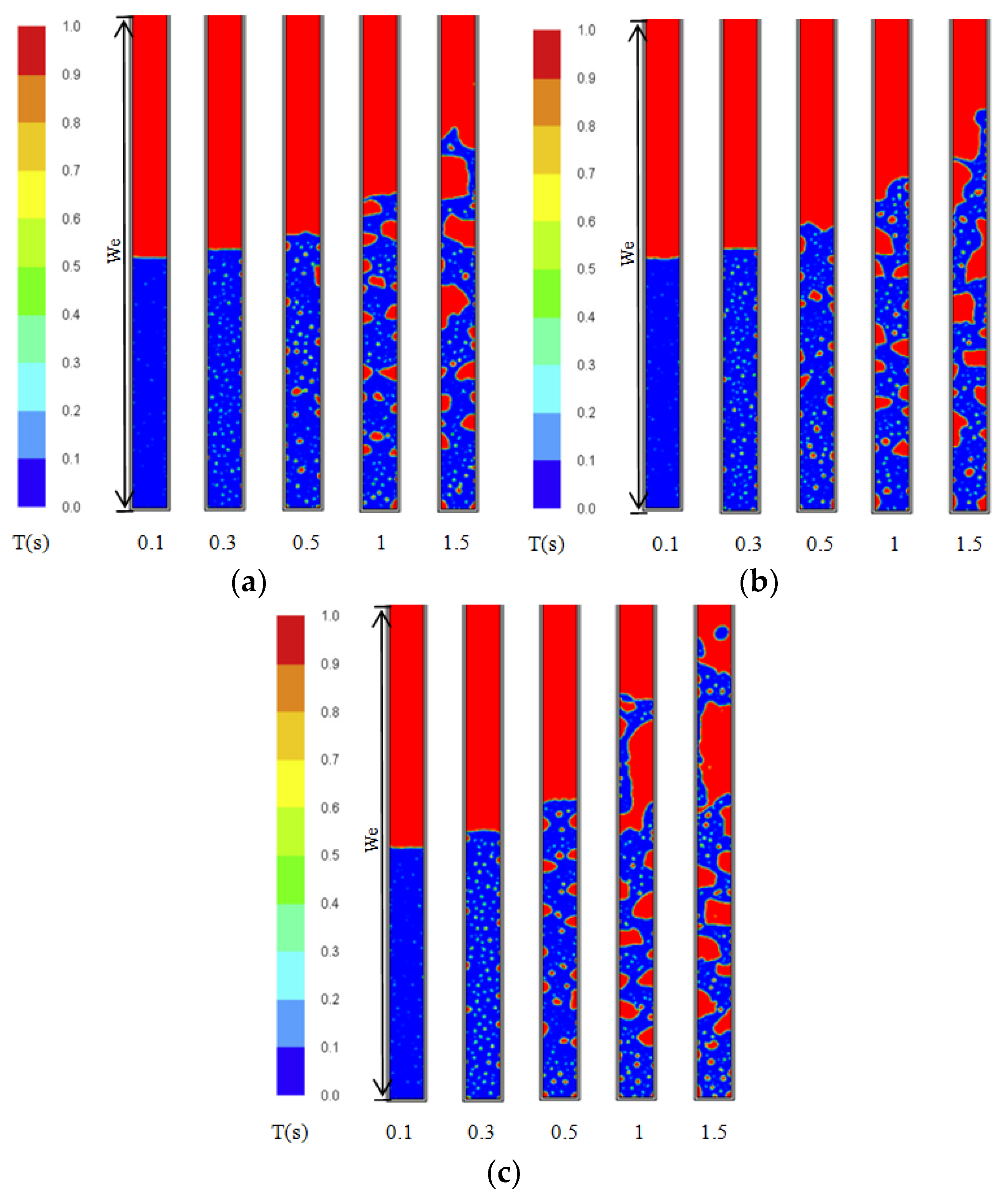
Pool boiling and vapor-liquid distribution in the evaporator section and the liquid film in the lower region of the condenser section are visualized in
Figure 4 and
Figure 5, respectively. The blue color represents that the liquid volume fraction is 1, indicating that only liquid exists. As evidenced by the liquid volume fraction (value: 0) represented by the red color, only vapor exists. The evaporator section is represented by “We” in
Figure 4, 60% of which is occupied by the liquid pool at 0.1 s.
The heating power transferred the heat into the liquid pool through the walls of the evaporator section. Evaporation occurred at the nucleation site, where liquid reached the saturation temperature at 0.3 s. Vapor bubbles formed and departed from the inner walls of the evaporator section at 0.5 s. As the heating input increased, more vapor bubbles formed and then started to grow upwards and to coalesce, at 1s and 1.5 s respectively. Finally, the vapor bubbles rose up to the interface between the liquid phase and vapor phase, where they broke up and passed the vapor phase. Moreover, the quantities, size, and shape of the vapor bubbles changed along with the heating input.
Conversely, saturated vapor condensed when it rose up to the condenser section through the adiabatic section. The adiabatic and condenser sections are represented by “Wa” and “Wc” in
Figure 5. Condensed liquid film formed on the inner walls of the condenser section, where heat was transferred to the external environment. At the beginning, the film was discontinuous at 5 s, 6 s, 7 s, and 8 s, and the heating input was 40 W (
Figure 5a). Based on continuous transportation of vapor from the evaporator section, more liquid was condensed on the inner walls of the condenser section. Eventually, at the heating input of 40 W, a continuous liquid film formed (visualized in
Figure 5a) at 9 s and 10 s, and it returned to the liquid pool of the evaporator section through the adiabatic section under gravity.
Apparently, the time required by the formation of a continuous liquid film is shortened by increasing the heating input power. Meanwhile, the thickness of the liquid film is increased by raising the heating input power at 10 s. More vapor appears and reaches the condenser section with rising heating input power, which increases the condensed liquid and accelerates the formation of a continuous liquid film. The simulation results prove that this numerical model can reproduce the difference in pool-boiling and film-wise condensation between different heating inputs.
5.2. The Wall Temperature Profile of the Numerical Simulation of the Thermosyphon
The average wall temperatures, versus time, for evaporator, adiabatic, and condenser sections are specified in
Figure 6. With a rising power input, the average wall temperature of the evaporator section increased between 0 s and 19 s (
Figure 6a). By the heat dissipation of the condenser section, the wall temperature of the evaporator section was relatively constant after 19 s, indicating that the thermosyphon needs 19 s to reach stable operation. The wall temperature of the evaporator also increased by elevating the heating input. Meanwhile, at the heating input of 80 W, its wall temperature volatility was also increased. Probably, geyser boiling, which was caused by the larger bubbles in
Figure 4c, reduced the stability of the thermosyphon. Compared to the evaporator section, the average wall temperature of the adiabatic section barely varies (
Figure 6b). Therefore, the center temperature of the adiabatic section can be specified as the saturation temperature of the thermosyphon.
As shown in
Figure 6c, the average wall temperature of the condenser section temporarily decreased from 0 s to 4 s at the heating input of 40 W and 60 W, because a constant heat flux boundary condition was applied on the walls of the condenser section at the beginning of the numerical simulation. The heat of the vapor phase region was transferred to the external environment while that generated by boiling had not yet been transferred to the condenser section. The average wall temperature of the condenser section began to increase when the heat generated by boiling started after 4 s at the heating inputs of 40 W and 60 W. Therefore, this thermosyphon started to work at 4 s at the heating inputs of 40 W and 60 W. In addition, the condenser section started to increase at 3 s at the heating input of 80 W, suggesting that the thermosyphon can work in advance by increasing the heating input.
5.3. The Thermal Resistance of the Numerical Simulation of the Thermosyphon
The thermal resistance of the whole thermosyphon can be defined as follows:
where
and
are the average wall temperatures of the evaporator and the condenser, respectively, and
represents the power input of the evaporator. Based on
Figure 7, the thermal resistance increases with extended time and then gradually levels off. In addition, the minimum of thermal resistance is 0.552 K/W, and its decrease is slowed down with increasing heating input (
Table 1).
and
have the following forms:
where R
40, R
60, and R
80 represent the thermal resistances at the heating inputs of 40 W, 60 W, and 80 W, respectively. The thermosyphon thermal resistances at various power inputs have been compared in this paper; the thermosyphon thermal resistance gradually decreased by increasing the power inputs.
5.4. The Effective Thermal Conductivity of the Numerical Simulation of the Thermosyphon
To evaluate the thermal performance of the thermosyphon filled with working fluid, the heat transfer capability is treated as a solid cylinder with equal size. The thermal conductivity of this solid cylinder is specified as the effective one of the thermosyphon with the following correlation:
where
,
, and
are the lengths of the total thermosyphon, evaporator, and condenser respectively;
and
are the outer diameter and inner diameter respectively; and
is the thermal conductivity of the wall.
and
represent the heat transfer coefficients of the evaporator and the condenser with the following forms, respectively:
where
and
are the average wall temperatures of the evaporator and the condenser, respectively, and
represents the power input.
The effective thermal conductivity, versus time, is displayed in
Figure 8. Apparently, it is highest initially, and it then decreases with prolonged time. Eventually, the effective thermal conductivity hardly fluctuates. As shown in
Table 2, with
and
calculated by (17-1) and (17-2), the effective thermal conductivity increases to a maximum (2.07 × 10⁶ W/m∙K
−1) with the rising of the heat flux, but the increment amplitude changes little.
where
,
, and
represent the thermal resistances at the heating inputs of 40 W, 60 W, and 80 W, respectively.
6. Conclusions
A transient two-dimensional model was built with the VOF technique to simulate the complex phenomenon in a thermosyphon. In order to calculate the heat and mass transfer, UDFs were associated with the governing equations of FLUENT by source terms. The CFD results confirmed that this model managed to reproduce pool boiling in the evaporator section and the formation of liquid film in the condenser section during the start-up of thermosyphon. Moreover, the simulation results showed that the quantities, size, shape, and position of vapor bubbles produced by boiling in the evaporator changed along with the heating power at the same time. With rising heating power, the time required by the formation of continuous liquid film was shortened, and the thickness also increased.
The average wall temperatures for condenser, adiabatic, and evaporator sections were investigated at different heating inputs during the operation of the thermosyphon. The prediction results showed that the thermosyphon reached a steady state after 19 s. Variations of the condenser wall temperature suggested that the heat pipes filled with pure water started to work in advance at appropriate heating power, which was around 3 s in the fastest case. We can increase heating power properly to reduce the start-up time and increase the effective thermal conductivity of the thermosyphon.
The thermal performance of the thermosyphon was evaluated by studying the thermal resistance and effective thermal conductivity. With increasing heating power, the thermal resistance decreased to a minimum value (0.552 K/W), whereas the effective thermal conductivity rose to a maximum (2.07 × 10⁶ W/m∙K).


