A New Method for Determining the Connection Resistance of the Compression Connector in Cable Joint

Abstract

The compression connector of a cable joint is one of the major components causing joint overheating. This paper proposed a new model to determine the connection resistance of the compression connector. It innovatively integrated electrical contacts model analysis (ECMA) with finite element analysis (FEA) in the modeling. The compacted stranded structure of the cable conductor was taken into account in the proposed model. The streamline distortion effect on the connection resistance was also established. To verify the applicability of the proposed model, the connection resistances of five compression connectors with different cross sections were measured. The modeling results and measurement results were in close agreement with each other.

1. Introduction

Cable joints are the weakest links in a cable system and its failure is mainly due to internal overheating [1,2,3,4]. In a cable joint, the highest temperature normally occurs in its compression connector [5]. If the compression connector has a considerably large connection resistance, a large quantity of heat can be generated, causing local overheating in the cable joint. Since the compression connector is totally sealed inside the cable joint, its condition is difficult to monitor during cable operation. It is thus necessary to investigate how to determine the connection resistance of the compression connector based on its structure parameters.

The connection resistance of the compression connector mainly consists of two parts. One is the volume resistance, which appears in the contact area of the cable conductors and the ferrule. Since this part volume resistance is affected by the “streamline effect”, it is referred to as “SE resistance” in this paper (refer to Section 4 for details). The SE resistance can be calculated by the characteristics of streamline distortion resistance [6,7]. The other part is the contact resistance between the cable conductors and ferrule which contributes most of the overall connection resistance. In the remainder of this paper, the focus will be on the determination of the contact resistance.

A number of methods have been employed to calculate the contact resistance in the literature including finite element analysis (FEA), experimental measurement, and electrical contacts model analysis (ECMA) [8,9,10,11,12,13,14,15,16,17,18,19,20,21,22,23,24,25,26]. In the FEA method, some researchers have added an extremely thin film on the contact interface of the two connectors. The actual contact condition was then simulated by changing the material properties of the film [8,9]. Other researchers have adopted a number of tiny conductive bridges on the contact interface to simulate the contact condition [10,11,12]. The electric-thermal coupling model of the cable joint was also established for assessing its hot spot and ampacity [13,14].

However, in the above methods, the stranded conductor was simplified as a single cylinder to save computing resources and pursue convergence [11,13,14,15]. To attain an accurate calculation of connection resistance, it is necessary to fully consider the stranded and compressed structure of the cable conductor, the local plastic deformation of the ferrule, and the actual contact interface between the ferrule and the cable conductor. In particular, the actual contact interface is extremely complex, which cannot be directly approximated by adding tiny geometry in a finite element model.

Though the initial connection resistance can be measured, the contact interface topography cannot be obtained from it. As a consequence, we could not investigate and analyze the defects and weak links in the manufacturing process of the compression connector nor could we propose an optimal crimping scheme. The ECMA method has been widely used to calculate contact resistance. It is worth investigating the suitability of applying ECMA to calculating resistance in the context of the compression connector of the cable joint.

The ECMA method has evolved from the macroscopic to microscopic scale and from elastic to plastic deformation [16,17,18]. Within the contact between two metals, the actual contact area is normally only a few contact spots. Holm et al. pointed out that the contact resistance was comprised of constriction resistance and film resistance of the whole contact spot [19]. Hertz et al. established a model considering the macroscopic elastic deformation [20]. Bickel et al. approximated the asperities on the rough contact surface as spherical shapes with their heights following a normal probability density function (Gaussian distribution) [21]. Based on this approximation, Greenwood and Williamson proposed a rough surface contact model assuming the asperities were elastically deformed [22]. Copper et al. suggested that plastic deformation could still occur on asperities of rough surface at very low contact pressures. They demonstrated the relationship between microhardness and the contact area of asperities [23]. Bahrami et al. also pointed out that the asperities had a high chance of being subjected to plastic deformation since the contact pressure on the asperities was concentrated on a small radius of curvature. Subsequently, Bahrami et al. proposed a model based on nonconforming rough surfaces [24,25,26]. To the best of the knowledge of the authors of this paper, the ECMA method has not been used in calculating the contact resistance in cable joints, however, it would be appropriate to integrate the ECMA with FEA to calculate the contact resistance.

In this paper, a new model was established to determine the connection resistance of the compression connector in the cable joint. The model combined the ECMA for nonconforming rough surface and the FEA for the structure and electric fields. Moreover, the model fully considered the stranded compacted structure of the cable conductor and the manufacturing process of the compression connector. Using the proposed model, the distribution of the radial equivalent stress field and radial displacement field on the contact interface between the ferrule and the cable conductors were determined. The contact resistance of the contact interface was also obtained. Furthermore, a simplified finite element model of the electric field under the influence of streamline distortion effects was also established for determining SE resistance. Finally, the connection resistance of five compression connectors with five different cross sections were measured. The effectiveness of the proposed model was then evaluated by comparing the modeling results with measurement results.

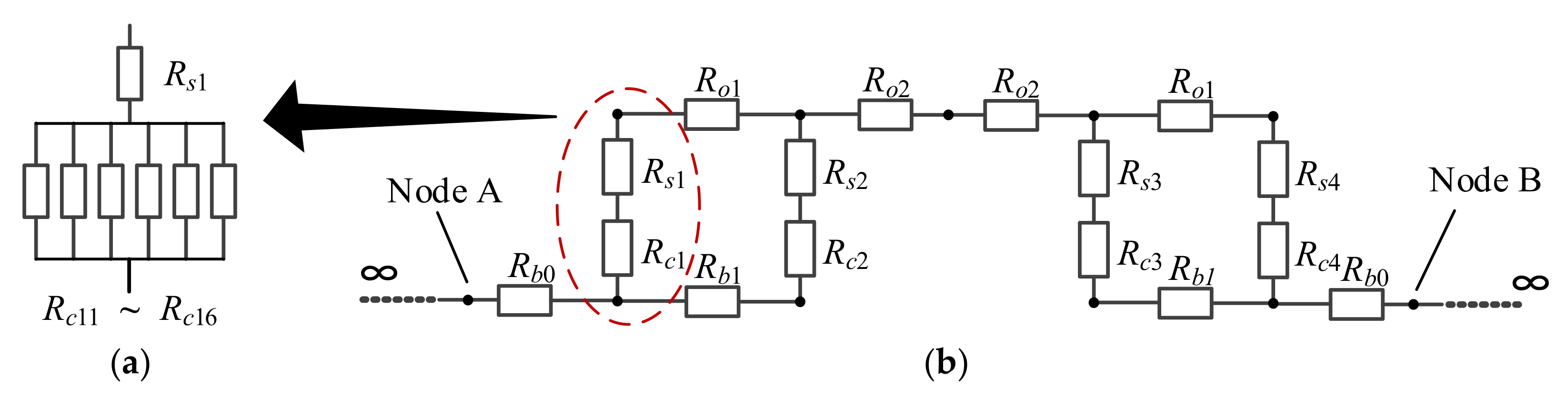
The paper is organized as follows. Section 2 establishes the equivalent circuit of the connection resistance of the compression connector. Section 3 and Section 4 develop models for determining the contact resistance and SE resistance, respectively. Section 5 presents the numeric results and analysis. Section 6 presents the experimental verification. Section 7 concludes the paper.

2. Circuit Model for Connection Resistance of Compression Connector

2.1. Cable Joint Crimping Process and Its Structure Model

A typical compression connector in the cable joint is shown in Figure 1. It is made of two cable conductors and one ferrule through a mechanical crimping process. The cable conductor is a type of round compacted stranded conductor (Figure 1a). Due to the effect of compacting, the cross section of each wire has an irregular shape and the gaps between these wires are partially filled. The ferrule is a cylindrical sleeve (Figure 1b). The crimping die consists of upper and lower dies and its internal shape is a regular hexagon with round corners (Figure 1c). The material of the cable conductor and the ferrule are copper and the crimping die is steel.

Before the crimping process, the two conductors are inserted into the ferrule and make contact with each other. During the crimping process, the hexagonal die acts radially on the surface of the ferrule. When the upper and lower dies are contacted, the crimping process is completed. The ferrule is crimped four times. After the crimping process, an air gap may still exist between the two cable conductors (Figure 1b). In the following, the gap was assumed to be 4 mm. In the figure, A and B are the two points for calculating the connection resistance of the compression connector.

2.2. Assumptions

To establish the circuit model for calculating the connection resistance of the compression connecter shown in Figure 1b, the following assumptions were made.

(1)

The compression connector’s structure is symmetrical. The position and sequence of crimping follow the industry standard during the manufacture of the compression connector (GB/T 14315).

(2)

The material of the compression connector was isotropic. Both stress relaxation and creep deformation were ignored.

(3)

The material of the compression connector was bilinear isotropic hardening.

(4)

The asperities on contact interface had a spherical shape and their heights followed a Gaussian distribution. The deformation of each asperity was plastic and independent.

2.3. Equivalent Circuit of the Compression Connector

The total resistance in each crimping area of the compression connector consists of a contact resistance and a SE resistance. Based on the positions of the crimping areas and the current path from the cable conductor to the ferrule, a circuit model for the connection resistance of the compression connector was established and is shown in Figure 2.

In Figure 2b, nodes A and B denote the left and right ends of the ferrule; R_b0 and R_b1 denote the AC resistances of the cable conductor in the non-crimping areas; R_o1 and R_o2 denote the resistances of the ferrule in the non-crimping areas; R_c1, R_c2, R_c3, and R_c4 denote the contact resistances in the crimping areas, and R_s1, R_s2, R_s3, and R_s4 denote the SE resistances in the crimping areas. The hexagonal die, the ferrule, and the cable conductor have an interference fit, and the crimping each time creates six independent contact areas between the ferrule and the cable conductor (each of the six contact areas is referred to as the “C-Area”). Therefore, R_c1, R_c2, R_c3, and R_c4 each consists of six contact resistances in parallel (each of them is referred to as the “C-Resistance”). As an example (Figure 2a), R_c1 is the sum of R_c11–R_c16 in the parallel connection. In addition, the connection resistance is the equivalent resistance between circuit nodes A and B.

Figure 3 shows the cross section diagram of the compression connector before and after crimping. R_c12 and R_c15 are formed by crimping the two center-surfaces of the upper and lower dies, while R_c11, R_c13, R_c14, and R_c16 are formed by crimping the four side-surfaces of the dies.

The contact resistance modeling is presented in Section 3 and the SE resistance modeling is presented in Section 4.

3. Modeling and Calculation of Contact Resistance

This section details the contact resistance modeling. Section 3.1 presents the basic contact model of nonconforming rough surface. Section 3.2 and Section 3.3 are derivations for determining contact resistance. Section 3.4 presents the theoretical formulations and boundary conditions for FEA. Finally, in Section 3.5, a generalized procedure for calculating the contact resistance is presented.

3.1. Contact Model of Nonconforming Rough Surfaces

Since the geometry of waviness and the gaps of macroscopic contacting surfaces of the C-Area are complicated, some simplifications needed to be made. Hertz [20], Clausing and Chao [27], Yovanovich [28], Nishino et al. [29] and Lambert [30] developed a number of simplified approaches where the complicated geometry of nonconforming rough contacts was simplified as the contact between an equivalent truncated rigid spherical and an equivalent flexible rough flat. Bahrami et al. further improved the Greenwood model. By using the plastic contact model proposed by Cooper, Bahrami introduced a plasticity index and local microhardness to describe the plastic deformation of the asperities. The Bahrami’s contact model for nonconforming rough surfaces is shown in Figure 4. In this paper, this model was used for calculating the C-Resistance.

In Figure 4, r is the distance from the geometric centerline of the rigid sphere; H_mic, σ and m are the microhardness, equivalent roughness, and equivalent asperity slope, respectively, and E′ is the equivalent elastic modulus. The normal displacement of the flat can be calculated from [22,31]:

$${\omega }_b(r)=\{\begin{array}{l}\frac{2}{E^{\prime }}{\displaystyle {\int }_0^{a_L}P(s)ds\hspace{0.17em}\hspace{0.17em}\hspace{0.17em}\hspace{0.17em}\hspace{0.17em}\hspace{0.17em}\hspace{0.17em}\hspace{0.17em}\hspace{0.17em}\hspace{0.17em}\hspace{0.17em}\hspace{0.17em}\hspace{0.17em}\hspace{0.17em}\hspace{0.17em}\hspace{0.17em}\hspace{0.17em}\hspace{0.17em}\hspace{0.17em}\hspace{0.17em}\hspace{0.17em}\hspace{0.17em}\hspace{0.17em}\hspace{0.17em}r=0}\\ \frac{4}{\pi E^{\prime }r}{\displaystyle {\int }_0^{r}sP(s)K(\frac{s}{r})ds\hspace{0.17em}\hspace{0.17em}\hspace{0.17em}\hspace{0.17em}\hspace{0.17em}r>s}\\ \frac{4}{\pi E^{\prime }}{\displaystyle {\int }_r^{a_L}P(s)K(\frac{r}{s})ds\hspace{0.17em}\hspace{0.17em}\hspace{0.17em}\hspace{0.17em}\hspace{0.17em}\hspace{0.17em}\hspace{0.17em}r<s}\end{array}$$

(1)

where ω_b(r) is the local bulk deformation; K(·) is the complete elliptic integral of the first kind; P(·) is the pressure distribution at the contact interface; s is a dummy variable; and a_L is the real contact radius. The equivalent spacing Y(r), which is the distance between the flexible flat and the rigid spherical in discrete element from the centerline r, can be calculated from:

$$Y(r)={\omega }_b(r)-u_0+r^2/2\rho$$

(2)

where ρ is the effective radius of curvature and u₀ is the maximum indentation of the sphere profile.

3.2. Calculation of Contact Resistance

Due to the surface cleaning techniques and the fracture of the surface film during crimping, the film resistances in the C-Areas can be ignored and only the constriction resistance was considered. The contact resistance was calculated from:

$$R_{cij}=\frac{{\rho }^{\prime }}{4{\displaystyle {\int }_0^{a_L}{a}_s(r)n_s(r)dr}}$$

(3)

where i = 1, …, 4, j = 1, 2, … 6; ρ′ is the material resistivity; a_s(r) is the mean radius of asperities in discrete element; and n_s(r) is the number of asperities in discrete element. a_s(r) and n_s(r) can be calculated from [23]:

$$\{\begin{array}{l}{a}_s=\sqrt{8/\pi }(\sigma /m)\exp (\lambda {(r)}^2)erfc\lambda (r)\\ n_s=0.0625(m/\sigma )[\exp (-2\lambda {(r)}^2)/erfc\lambda (r)]A_a\\ A_r/A_a=0.5erfc\lambda (r)\end{array}$$

(4)

where λ(r) is the characteristic function of the contact gap on rough surface, λ(r) = Y(r)/1.41σ, erfc() is the Gaussian error function complement; A_a is the apparent contact area; and A_r is the real contact area. The relationship between roughness σ and surface slope m can be obtained as per [30]:

$$m=0.076{\sigma }^{0.52}.$$

(5)

Since the actual contact surface is not smooth, the stress distribution and actual contact radius are deviated from the Hertz contact. The surface roughness has an impact on the macroscopic contact model in that the apparent contact area with a larger radius leads to a smaller maximum contact stress. The maximum pressure P₀ and contact radius a_L can be calculated from [24]:

$$\{\begin{array}{l}{P}_0^{}=1/(1+1.37\alpha {\tau }^{-0.075})\\ a_L^{}=1.80\sqrt{a+0.31{\tau }^{0.056}}/{\tau }^{0.028}.\end{array}$$

(6)

3.3. Cable Conductor Modeling and Apparent Contact Area Calculation

The cross section of the uncompacted stranded conductor of cable is shown in Figure 5. After twisting the conductors, the compression of the conductor must be performed by a circular die. The deformation of the round compacted stranded conductor in different layers is shown in Figure 6, where the shadow A is used to fill the shadow B; r₁ is the radius of the solid wire; and r₂, r₃, and r₄ are the radius of the excircle of the second, third, and fourth layer solid wires after compression. From Figure 6, it was reasonable to assume that there was no deformation of the first-layer solid wire and the deformation of the solid wires in other layers occurred approximately in two concentric circles.

On the assumption that the deformation of the conductor in different layers was consistent, the radius can be calculated from:

$$\{\begin{array}{l}{D}_1=(2n-1)d\\ D_2=d[{(k/\mu \eta )}^{1/2}]\\ d_{\mathrm{c}}=d-(D_1-D_2)/2(n-1)\end{array}$$

(7)

where D₁ is the external diameter of the stranded conductor before compaction; D₂ is the external diameter of the stranded conductor after compaction; d_c is the difference of radius between the inscribed circle and the excircle in any layer; n is the number of layer; d is the diameter of solid wire; k is the total number of solid wires; μ is extension coefficient; and η is the compaction coefficient. The cable conductor with a 240 mm² cross section is taken as an example. The calculated parameters of this conductor are shown in

Table 1. The results of the cable conductor with 240 mm² cross section.

Parameters	n	k	μ	η	d	D1	D2	dc
Value/mm	4	37	0.89	1.12	2.96	20.72	18.03	2.52

.

From Table 1, it can be seen that the deformation of a single-layer was small, that is, the area of shadow A was unable to fill shadow B (Figure 6a). Therefore, for the cable conductor, the actual contact length could be approximated by the arc length where the excircle intersects the solid wires (Figure 7). In Figure 7, |o₁a| is the radius of inscribed circle, |o₁c| is the radius of excircle, |o₂a| is equals to |o₂e|, and |o₂b| is the radius of solid wire.

According to Figure 7 and Equation (9), the actual contact length (l_e) of the solid wire in the C-Areas can be calculated from:

$$l_{\mathrm{e}}=\arcsin (\frac{\sqrt{d^2-d_{\mathrm{c}}^2}}{D_2})\times \frac{\pi D_2}{180}.$$

(8)

Thus, the apparent contact area of the cable conductor and the ferrule in the C-Area can be calculated from:

$$A_{\mathrm{s}}={\displaystyle \sum _{i=1}^q{l}_{\mathrm{e}}\sin \alpha \times l_i}$$

(9)

where q is the number of outer-layer solid wires of the cable conductor in the C-Area; α is the helix angle of the outer-layer stranded solid wires; and l_i is the contact length of the i-th solid wire, i = 1, …, q.

3.4. Structure Field Control Equations and Boundary Conditions

The finite element control equations of three-dimensional solid mechanics is established. The displacement component can be calculated by the equilibrium differential equation and boundary conditions. The stress components can be calculated by the geometric equation. The stress components can be calculated by the physical equation. Each point has three degrees of freedom (DOF) of displacement, i.e., u, v, and w. The control equation is as follows:

$$\{\begin{array}{l}(\lambda +G)\frac{\partial e}{\partial x}+G{\nabla }^{2}u+X_N=0\\ (\lambda +G)\frac{\partial e}{\partial y}+G{\nabla }^{2}v+Y_N=0\\ (\lambda +G)\frac{\partial e}{\partial z}+G{\nabla }^{2}w+Z_N=0\end{array}$$

(10)

where λ is the lame constant; G is the shear modulus; and e is the volumetric strain.

The hexagonal die was considered as a rigid body, and both the cable conductor and ferrule were considered as flexible bodies. All DOFs of displacements on both sides of the cable conductor were constraints. The radial and axial displacement of hexagonal die were set according to the industry standard (GB/T 14315). Axial friction during crimping was ignored.

3.5. Calculation Method of Contact Resistance

The flowchart of calculating contact resistance using the results in Section 3.2, Section 3.3 and Section 3.4 is shown in Figure 8. First, the equivalent physical model of the round compacted stranded conductor was established (refer to Section 3.3). The finite element model of the compression connector before crimping was established based on this model. The contact stress F(r) and macroscopic deformation ω_b(r) of the contact interface after crimping were obtained by the FEA. Then, the macroscopic deformation was substituted into the contact model of nonconforming rough surfaces. The number and radius of contact spots in the C-Area and the contact reaction force F_k(r) were calculated. If |F_k(r) − F(r)|/F(r) was less than 5%, then F(r) = F_k(r) and the above iterative process could be terminated and the result was the contact resistance; otherwise, the iterative process continued.

4. Model and Calculation of Streamline Effect (SE) Resistance

4.1. FEM Analysis for the Overlap Joint without Contact Interface

The schematic for the overlap joint without contact interface is shown in Figure 9. When the current flowed through the overlap, the current line was distorted. As a result, even if it was perfectly overlapped (no contact resistance), its resistance was still higher than that of a conductor of the same length. This is called the “streamline effect.” In the figure, t is the conductor thickness; l is the overlap length; and distance AB = BC.

Melsom and Booth conducted extensive experiments on overlapping joint at different overlapping lengths and plotted the curve of resistance ratio [6]. According to the curve, the resistance of the conductors affected by streamline can be calculated, i.e., the resistance R_AB in Figure 9. To verify the feasibility of analyzing the streamline effect by FEA, the finite element model of the electric field was established based on the experiments of Melsom and Booth. The results of the FEA and the experiment are shown in Figure 10. k is the resistance ratio, which represents the ratio of resistance R_AB of the overlap region to the resistance R_BC of the conductor of the same length. The results show the curves, which had very good agreement.

4.2. Calculation of SE Resistance

It was assumed that the ferrule and the cable conductor were in perfect contact in the C-Area (no contact resistance). Under this condition, the contact properties of the compression connector were similar to those of the overlap joint without contact interface. The cross-sectional geometry model of the compression connector without contact interface is shown in Figure 11 (only half axis is shown due to symmetry).

In the figure, d_c is the radius of cable conductor, d_f is the thickness of the ferrule, m₁ is the distance from the edge of the ferrule to the indentation, m₂ is the distance between one indentation and another adjacent indentation, m₃ is the axial thickness of the hexagonal die cavity, and distance AB = CD = MA. When the AC current flows in from point M, the path of the current line is shown by the arrow in Figure 11.

The geometric model was applied to the FEA of a two-dimensional electric field. Current was applied to one end of the conductor and the other end was set to ground (red line in Figure 11). The current density distribution and voltage distribution of the compression connector could be obtained and the SE resistance ratios can be calculated from:

$$\{\begin{array}{l}{k}_1=U_{AB}/U_{MA}\\ k_2=U_{CD}/U_{MA}\\ k_3=U_{D_1{C}_1}/U_{MA}\\ k_4=U_{B_1{A}_1}/U_{MA}\end{array}$$

(11)

where k₁, k₂, k₃, and k₄ are the SE resistance ratios between A and B, C, and D, D₁ and C₁, B₁, and A₁, respectively. $U_{AB}$, $U_{CD}$, $U_{D_1{C}_1}$, $U_{B_1{A}_1}$, and $U_{MA}$ are the voltages between A and B, C, and D, D₁, and C₁, B₁, and A₁, M and A, respectively. Then, the SE resistances can be calculated from:

$$R_{si}=k_i{m}_3{R}_b\times {10}^{-3}$$

(12)

where k_i is the SE resistance ratio, i = 1, 2, 3, 4; R_b is the AC resistance of cable conductor per unit lengths. R_b can be calculated from:

$$\{\begin{array}{l}{R}_b=R^{\prime }(1+Y_s+Y_p)\\ R^{\prime }=R_0\times [1+{\alpha }_{20}(\theta -20)]\\ Y_s=x_s^4/(192+0.8x_s^4)\\ x_s^2=8\pi f/R^{\prime }\times {10}^{-7}{k}_s\end{array}$$

(13)

where R′ is the direct current (DC) resistance of the conductor at operating temperature; R₀ is the DC resistance of the conductor at 20 °C; α₂₀ is the temperature coefficient of the conductor material at 20 °C; θ is the operating temperature of the cable conductor; Y_S is skin effect coefficient; and Y_P is the proximity effect coefficient; and f is the power frequency.

In the FEA for the electric field, the compacted stranded structure of the cable conductor, the skin effect and the complexity of the contact interface were ignored. The reasons are as follows:

(1)

Copper is a non-ferromagnetic material, and the skin effect has less effect.

(2)

The compacted stranded structure of the cable conductor helps to reduce the skin effect. As for the cable with a 240 mm² cross section, the relative error between the AC resistance values with and without considering the skin effect was only 1.133% according to the IEC 60287.

(3)

The SE resistance is only a small part of the connection resistance and its approximation does not affect the accuracy of the total resistance.

5. Numeric Experiment Results and Analysis

5.1. Parameters for Numeric Experiments

In this section, the connection resistances of five different cross section compression connectors were calculated. The compression connector with a 240 mm² cross section was taken as an example in discussion. Its geometric parameters are shown in

Table 2. Structure parameters of the 240 mm² cross section compression connector.

Parameters	Value
Solid wire diameter (mm)	2.96
Total number of solid wires (mm)	37
The length of lay of the strands in outer layer (mm)	145.4
Extension coefficient	0.89
Compaction coefficient	1.12
Ferrule inner diameter (mm)	20.04
Ferrule outer diameter (mm)	27.14
Ferrule length (mm)	109.62
Die cavity outer diameter (mm)	28.0
Die cavity round corner (mm)	2.5

. The parameters for calculating the contact and SE resistance are shown in

Table 3. Parameters for calculating the contact and streamline effect (SE) resistance.

Parameters	Value
Ferrule/Cable conductors roughness (μm)	6.3/4.0
Ferrule/Cable conductors young’s modulus (GPa)	121
Ferrule/Cable conductors poisson’s ratio	0.31
Ferrule/Cable conductors yield strength (GPa)	0.32
Ferrule/Cable conductors tangent modulus (GPa)	1.1
Density of copper (g/cm3)	8.9
Resistivity of copper (Ω·m)	1.75 × 10−8
Current of FEA of electric field (kA)	10
Frequency (HZ)	50
Distance from the edge of the ferrule to the indentation (mm)	4.12
Distance between one indentation and another adjacent indentation (mm)	6.04
Axial thickness of the hexagonal die cavity (mm)	16.0

.

5.2. Mesh Generation

The ANSYS software is a large-scale general-purpose FEA software that integrates structure, fluid, electric field, magnetic field and sound field analysis. It can interface with most computer aided design (CAD) software to realize data sharing and exchange. In this paper, it was used to investigate the structure field and electric field of the compression connector. The hexahedral or quadrilateral meshes were applied in the FEA as much as possible. The mesh diagrams of the FEA of the structure field and electric field are shown in Figure 12. The structure field contained 509,756 elements and 126,665 nodes (Figure 12a). The electric field contained 38,096 elements and 188,633 nodes (Figure 12b).

5.3. Results and Analysis

The radial displacement of the compression connector after crimping was computed and shown in Figure 13. Figure 13a shows that the radial displacement field of the outer surface of the ferrule from the front view of the upper die. The maximum radial displacement of each indentation was near the centerline of the indentation. The deepest indentations were those formed by crimping the two center-surfaces of the upper and lower dies (the four deepest indentations show in Area 1 in Figure 13a). The convex areas appeared in the edge of the ferrule (Area 2 in Figure 13a). The calculated interference fit between the hexagonal die and the ferrule was 1.475 mm, which was slightly larger than the maximum depth of the indentations, which was 1.453 mm. This is because the elastic deformation of the indentations could recover after the crimping (i.e., elastic resilience).

Figure 13b shows the radial displacement field of the inner surface of the ferrule from the front view of the upper die. The convex shapes formed by crimping the two center-surfaces of the upper and lower dies had the highest convex (Area 3 in Figure 13b). According to the stereogram (left side graph in Figure 13b), which enlarged the original radial displacement by four times, the complex shape of the convex body was approximately a truncated sphere. The calculated clearance fit between the ferrule and the cable conductor was 0.93 mm. As a consequence, only the part in Figure 13b with a radial displacement of more than 0.93 mm had contact with the cable conductor.

Figure 13c shows the radial displacement field on the surface of the two compacted stranded conductors. The C-Areas formed by crimping the two center-surfaces of the upper and lower dies were much deeper than others (Area 4 in the figure). Due to the gap between the solid wires of the outer layer, the maximum displacement was not continuous, as shown in the enlarged area (left side graph in Figure 13c).

Though the structure and the crimping position were symmetrical, the radial displacement of the compression connector was still not completely symmetrical, i.e., Area 1 in Figure 13a, Area 3 in Figure 13b, and Area 4 in Figure 13c. Such non-complete symmetry is caused by the law of constant volume and minimum resistance during the plastic deformation of metal. The direction of metal flow always tends to the direction of least resistance. The direction of metal flow during four times crimping is shown in Figure 14.

Larger radial deformation will result in greater radial stress. When the crimping was completed, the maximum stress occurred in the C-Areas formed by crimping the two center-surfaces of the upper and lower dies (Figure 15). According to the technical manual, the yield strength of copper was about 320 MPa, which was smaller than the maximum stress in Figure 15. As a consequence, plastic deformation occurred in the C-Areas.

The calculation results of contact resistance are shown in

Table 4. Calculation results of contact resistance (Unit: μΩ).

Parameters	Rc1	Rc2	Rc3	Rc4
Value	15.8	11.1	10.9	18.9

. It was obvious that the contact resistances R_c1 and R_c4 formed by crimping on two sides of the ferrule were slightly larger than the contact resistances R_c2 and R_c3 formed by the crimping at the middle of the ferrule.

R_c1 is made of six C-Resistances in parallel (R_c11–R_c16), and the calculation results are shown in

Table 5. Calculation result of C-Resistances (Unit: μΩ).

Parameters	Rc11	Rc12	Rc13	Rc14	Rc15	Rc16
Value	489.4	32.4	477.3	421.4	30.9	412.6

. From the table, it can be seen that the C-Resistances R_c12 and R_c15 formed by crimping the two center-surfaces of the upper and lower dies were much smaller than the other C-Resistances. Thus, the contact resistance R_c1 was determined by R_c12 and R_c15. In addition, the values of R_c12 and R_c15 were slightly different, which was due to the influence of gravity.

5.4. Calculation Results and Analysis of SE Resistance

The results of the FEA of the electric field are shown in Figure 16. Figure 16a shows the voltage distribution, and the values plotted on the graph correspond to the voltage at each node in Figure 11. According to Equation (13), the SE resistance ratios can be calculated (shown in

Table 6. Result of the SE resistance ratios.

Parameters	k1	k2	k3	k4
Value	0.755	1.034	1.034	0.755

).

The current density distribution is shown in Figure 16b. The current density distribution was nonuniform due to the influence of the “streamline effect” (Area 5 in the figure). The region with a large current density corresponded to k₂ and k₃ in Table 6, and the small current density corresponded to k₁ and k₄ in Table 6. The maximum value of the current density occurred at the crimp edge and is depicted as the red dotted circle in Figure 16b.

The calculation results of the SE resistances are shown in

Table 7. Result of SE resistance (Unit: μΩ).

Parameters	Rs1	Rs2	Rs3	Rs4
Value	1.03	1.41	1.41	1.03

. The value was far less than the contact resistances. Thus, it was concluded that the estimation of the SE resistance had little influence on the accuracy of the connection resistance.

6. Experimental Verification

The connection resistance of the compression connectors with five different cross sections were measured using IUXPower and a digital DC bridge. The compression connectors with 120, 150, 240, 500, and 630 mm² cross sections are shown in Figure 17a. Figure 17b shows the digital DC bridge, which can measure DC resistance and the measuring accuracy was ±0.01 μΩ. Figure 17c shows the IUXPower, which can apply a stable AC current and measure the AC resistance. The measurement setup is shown in Figure 17d. The measurement procedures are as follows:

(1)

The IUXPower supplies a 50 Hz, 200 A AC current to measure loop AC resistance.

(2)

The digital DC bridge was used to measure the DC resistance of the copper busbar. The measured copper busbar DC resistance was considered as equal to its AC resistance.

(3)

The connection resistance was obtained by twice deducting the DC resistance of the copper busbar from the loop AC resistance.

To ensure the reliability of the experimental results, all experiments were conducted at least twice with a standard deviation less than 3%. The measurement results and calculation results based on the four methods are shown in

Table 8. Connection resistance obtained from different methods (Unit: μΩ).

Section/mm2	Empirical Formula 1	Hertz 1	Greenwood 1	Bahrami 1	Experiment
120	255.1	108.2	99.5	87.4	90.8
150	117.2	60.8	54.6	45.9	47.1
240	61.2	32.5	29.6	24.8	25.2
500	32.4	20.6	19.2	13.4	14.0
630	28.2	14.3	13.4	8.7	9.4

¹ The numeric models were developed by using four different electrical contact models. For ease of discussion, the names of the electrical contact models were utilized for describing these new numerical methods.

.

In the table, the results of the empirical formula were derived from a large number of measurements [32]. The Hertz model ignores the microscopic contact between the conductors and the ferrule. The Greenwood model ignores the plastic deformation of the asperities. The Bahrami model considers the influence of microscopic contact, plastic deformation, and change of asperity summit radius, which results in a lower connection resistance. The average relative error of the four models is shown in

Table 9. Relative error of different methods.

Empirical Formula	Hertz	Greenwood	Bahrami
160.66%	35.29%	24.48%	3.95%

. Therefore, we can conclude that the Bahrami method can determine the connection resistance of the compression connector in the cable joint.

When the connection resistance is large, the local overheating can occur. Comparing the AC resistance of the cable conductor with the equal length of the ferrule, it was found that the resistance of the compression connector was much larger than that of the cable conductor. When the load was 300 A, the 120, 150, 240, 500, and 630 mm² cross section compression connector generated 24,375 J, 10,984 J, 4665 J, 2009 J, and 1134 J of additional heat per hour, respectively. The AC resistance and connection resistance of cable conductors are shown in

Table 10. Connection resistance of compression connector and AC resistance of cable.

Section/mm2	AC Resistance of Cable Conductor/μΩ		Connection Resistance/μΩ
	IEC 60287	Experiment
120	15.4	15.6	90.8
150	13.1	13.2	47.1
240	9.4	10.8	25.2
500	6.4	7.8	14.0
630	5.8	5.9	9.4

.

7. Conclusions

The main conclusions of this paper can be summarized as follows:

(1)

The new method proposed in this paper could accurately determine the connection resistance of the compression connector in the cable joint.

(2)

The connection resistance of the compression connector was much greater than that of the equal length cable conductor, and this was the main reason for the overheating.

(3)

The six parallel contact resistances formed by crimping the two center-surfaces of the upper and lower dies were much smaller than that formed by the other surfaces.

(4)

The contact resistances formed by four times crimping were not equal due to the law of constant volume and minimum resistance during the metal plastic deformation. The contact resistances formed in the middle of the ferrule were larger than that formed in two sides. The total contact resistance contributed most of the overall connection resistance.

(5)

The current line distortion (streamline effect) had little effect on the connection resistance.

In the future, more work will be devoted to assessing the connection resistance of the compression connector under different manufacturing processes that occur in actual engineering. Finding the optimal scheme is of great significance.

References

1. Ruan, J.; Liu, C.; Huang, D.; Zhan, Q.; Tang, L. Hot spot temperature inversion for the single-core power cable joint. Appl. Therm. Eng. 2016, 104, 146–152. [Google Scholar] [CrossRef]
2. Fu, J.; Cheng, P.; Chen, W.; Hu, X.; Wang, Q.; Yang, Q.; Yang, F. Investigation of the effects of insulation defects on the 3-D electromagnetic-thermal coupling fields of power cable joint. In Proceedings of the IEEE Conference on Industrial Electronics and Applications, Hefei, China, 5–7 June 2016; pp. 1436–1439. [Google Scholar]
3. Liu, Y.; Liu, G.; Wang, Z.; Xu, T.; Xu, U. Experimental Analysis on Crimping Resistance of Connecting Pipe of Cable Intermediate Joint. Guangdong Electr. Power 2016, 29, 108–112. [Google Scholar]
4. Ruan, J.; Zhan, Q.; Tang, L.; Tang, K. Real-Time Temperature Estimation of Three-Core Medium-Voltage Cable Joint Based on Support Vector Regression. Energies 2018, 11, 1405. [Google Scholar] [CrossRef]
5. Yang, F.; Cheng, P.; Luo, H.; Yang, Y.; Liu, H.; Kang, K. 3-D thermal analysis and contact resistance evaluation of power cable joint. Appl. Therm. Eng. 2016, 93, 1183–1192. [Google Scholar] [CrossRef]
6. Melsom, S.W.; Booth, H.C. The efficiency of overlapping joints in copper and aluminium busbar conductors. J. Inst. Electr. Eng. 1922, 60, 889–899. [Google Scholar] [CrossRef]
7. Braunovic, M. Effect of connection design on the contact resistance of high power overlapping bolted joints. IEEE Trans. Compon. Packag. Technol. 2002, 25, 642–650. [Google Scholar] [CrossRef]
8. Laor, A.; Herrell, P.J.; Mayer, M. A Study on Measuring Contact Resistance of Ball Bonds on Thin Metallization. IEEE Trans. Compon. Packag. Manuf. Technol. 2015, 5, 704–708. [Google Scholar] [CrossRef]
9. Dhotre, M.T.; Korbel, J.; Ye, X.; Ostrowski, J.; Kotilainen, S.; Kriegel, M. CFD Simulation of Temperature Rise in High Voltage Circuit Breakers. IEEE Trans. Power Deliv. 2017, 32, 2530–2536. [Google Scholar] [CrossRef]
10. Qiang, R.; Rong, M. Simulation of the contact resistance of high voltage apparatus with the method of coupling contact surface. In Proceedings of the International Conference on Electric Power Equipment—Switching Technology, Matsue, Japan, 20–23 October 2013; pp. 1–4. [Google Scholar]
11. Liu, G.; Guo, D.; Wang, P.; Deng, H.; Hong, X.; Tang, W. Calculation of Equivalent Resistance for Ground Wires Twined with Armor Rods in Contact Terminals. Energies 2018, 11, 737. [Google Scholar] [CrossRef]
12. Li, X.; Qu, J.; Wang, Q.; Zhao, H.; Chen, D. Numerical and Experimental Study of the Short-Time Withstand Current Capability for Air Circuit Breaker. IEEE Trans. Power Deliv. 2013, 28, 2610–2615. [Google Scholar] [CrossRef]
13. Yang, F.; Liu, K.; Cheng, P.; Wang, S.; Wang, X.; Gao, B.; Fang, Y.; Xia, R.; Ullah, I. The Coupling Fields Characteristics of Cable Joints and Application in the Evaluation of Crimping Process Defects. Energies 2016, 9, 932. [Google Scholar] [CrossRef]
14. Wang, P.; Liu, G.; Ma, H.; Liu, Y.; Xu, T. Investigation of the Ampacity of a Prefabricated Straight-through Joint of High Voltage Cable. Energies 2017, 10, 2050. [Google Scholar] [CrossRef]
15. You, L.; Wang, J.; Liu, G.; Ma, H.; Zheng, M. Thermal Rating of Offshore Wind Farm Cables Installed in Ventilated J-Tubes. Energies 2018, 11, 545. [Google Scholar] [CrossRef]
16. Murashov, M.V.; Panin, S.D. Modeling of Thermal Contact Conductance. In Proceedings of the International Heat Transfer Conference, Washington, DC, USA, 8–13 August 2010; pp. 387–392. [Google Scholar]
17. Li, L.; Song, W.; Zhang, G.; Jia, D. An electrical contact resistance model including roughness effect for a rough MEMS switch. J. Micromech. Microeng. 2012, 22, 115023. [Google Scholar] [CrossRef]
18. Goedecke, A.; Jackson, R.L.; Mock, R. A fractal expansion of a three dimensional elastic–plastic multi-scale rough surface contact model. Tribol. Int. 2013, 59, 230–239. [Google Scholar] [CrossRef]
19. Holm, R. Electric Contacts: Theory and Application, 4th ed.; Springer: Berlin, Germany, 1979. [Google Scholar]
20. Johnson, K.L. Normal Contact of Elastic Solids: Hertz Theory; Cambridge University Press: Cambridge, UK, 1989. [Google Scholar]
21. Bickel, E. Some fundamental problems in the measurement of surfaces. In Proceedings of the International Production Engineering Research Conference, Washington, DC, USA, 17–19 January 1963. [Google Scholar]
22. Greenwood, J.A. The elastic contact of rough spheres. J. Appl. Mech. 1967, 34, 153. [Google Scholar] [CrossRef]
23. Cooper, M.G.; Mikic, B.B.; Yovanovich, M.M. Thermal contact conductance. Int. J. Heat Mass Transf. 1969, 12, 279–300. [Google Scholar] [CrossRef]
24. Bahrami, M.; Culham, J.R.; Yovanovich, M.M.; Schneider, G.E. Thermal Contact Resistance of Nonconforming Rough Surfaces, Part 1: Contact Mechanics Model. J. Thermophys. Heat Transf. 2004, 18, 218–227. [Google Scholar] [CrossRef]
25. Bahrami, M.; Culham, J.R.; Yananovich, M.M.; Schneider, G.E. Review of Thermal Joint Resistance Models for Nonconforming Rough Surfaces. Appl. Mech. Rev. 2006, 59, 411–431. [Google Scholar] [CrossRef]
26. Bahrami, M.; Culham, J.R.; Yananovich, M.M.; Schneider, G.E. Thermal Contact Resistance of Nonconforming Rough Surfaces, Part 2: Thermal Model. J. Thermophys. Heat Transf. 2004, 18, 218–227. [Google Scholar] [CrossRef]
27. Clausing, A.M. Thermal Contact Resistance in a Vacuum Environment. ASME J. Heat Transf. 1965, 87, 243. [Google Scholar] [CrossRef]
28. Yovanovich, M.M. Overall constriction resistance between contacting rough, wavy surfaces. Int. J. Heat Mass Transf. 1969, 12, 1517–1520. [Google Scholar] [CrossRef]
29. Nishino, K.; Yamashita, S.; Torii, K. Thermal contact conductance under low applied load in a vacuum environment. Exp. Therm. Fluid Sci. 1995, 10, 258–271. [Google Scholar] [CrossRef]
30. Lambert, M.A.; Fletcher, L.S. Thermal contact conductance of spherical rough metals. J. Heat Transf. 1996, 119, 684–690. [Google Scholar] [CrossRef]
31. Gladwell, G.M.L. Contact Problems in the Classical Theory of Elasticity; Sijthoff & Noordhoff: Rockville, MD, USA, 1980. [Google Scholar]
32. Xu, J.; Li, K. The Research on Resistance of Electrical Contact. Electr. Eng. Mater. 2011, 1, 10–13. [Google Scholar]
Figure 1. Structure of compression connector in cable joint. (a) Cross section of the cable conductor; (b) front view of the compression connector; and (c) 3D stereogram of the hexagonal die.
Energies 11 01667 g001
Figure 2. Circuit model of the compression connector in the cable joint. (a) Six contact resistances in parallel; and (b) equivalent circuit of connection resistance.
Energies 11 01667 g002
Figure 3. Cross section of compression connector: (a) before crimping and (b) after crimping.
Energies 11 01667 g003
Figure 4. Contact model for nonconforming rough surfaces [24].
Energies 11 01667 g004
Figure 5. Cross section of the uncompacted stranded conductor.
Energies 11 01667 g005
Figure 6. Deformation model of round compacted stranded conductors in different layers: (a) the second-layer; (b) the third-layer; and (c) the fourth-layer.
Energies 11 01667 g006
Figure 7. Actual contact length of the outer-layer compacted stranded conductor.
Energies 11 01667 g007
Figure 8. Flow chart of the calculation method of contact resistance.
Energies 11 01667 g008
Figure 9. Schematic of an overlap joint without contact interface [6,7].
Energies 11 01667 g009
Figure 10. Effect of current line distortion on the resistance of an overlapping joint.
Energies 11 01667 g010
Figure 11. The 1/2-axis cross-sectional geometry model of the compression connector without contact interface (gap refers to the air gap).
Energies 11 01667 g011
Figure 12. Mesh diagrams of the FEA: (a) structure field and (b) electric field.
Energies 11 01667 g012
Figure 13. Radial displacement distribution of compression connector: (a) outer surface of ferrule; (b) inner surface of ferrule; and (c) surface of compacted stranded conductors.
Energies 11 01667 g013
Figure 14. Displacement vector field of compression connector in four crimping processes: (a) first time; (b) second time; (c) third time; and (d) fourth time.
Energies 11 01667 g014
Figure 15. Radial stress distribution in C-Areas.
Energies 11 01667 g015
Figure 16. Results of FEA of electric field: (a) electric voltage; and (b) current density.
Energies 11 01667 g016
Figure 17. Experimental measurement of the connection resistance: (a) compression connectors with 120, 150, 240, 500, and 630 mm2 cross sections; (b) digital DC bridge; (c) IUXPower; and (d) experimental system and measurement method.
Energies 11 01667 g017