Integrated Full-Frequency Impedance Modeling and Stability Analysis of the Train-Network Power Supply System for High-Speed Railways

Abstract

To investigate the harmonic resonance, harmonic instability and low-frequency oscillation phenomena in high-speed railways, this paper proposes a full-frequency impedance model of the train-traction network system (simplified as ‘train-network’) based on d-q coordinates system. Compared with traditional models which deal with only the grid-side converter, the proposed model also includes its load models—the inverter and the traction motor. It also reflects complete control scheme of grid-side converter, which makes it easier to analyze unstable phenomena mentioned above. Moreover, this paper improves the impedance modeling of the network by taking the network impedance and admittance into detailed consideration. In addition, based on the proposed train-network model, the 3D figure and zero-pole diagram are also presented for the analysis of the stability of the integral system. Simulation and experiment results verify the accuracy of the model.

1. Introduction

Being developed rapidly, more and more high-speed trains (HSTs) have been put into service in China. According to reports, more than 1600 HSTs are now being used for passenger service [1]. Meanwhile, the power systems of high-speed railways face significant challenges, including the harmonic resonance, harmonic instability and low-frequency oscillation (LFO) phenomena noticed in recent years, which can hinder the normal operations of the trains. Based on the previous literature, these unstable phenomena in high-speed railway system can be summarized as follows:

• Harmonic Resonance

The frequency of harmonic resonance usually ranges from a few hundred Hertz to kilohertz. During the train operation, high-frequency harmonic components are generated because of the pulse-width modulation (PWM) switching action of the grid-side converter on the train. Such high-frequency components act as harmonic sources and then inject harmonics into the traction network. When the train is running, and if the harmonic frequency emitted by the grid-side converter in the train is in the range of the intrinsic frequency of the train-network system, the high-frequency harmonics will be amplified by resonance, hence harmonic resonance is initiated. Such amplified resonant currents and voltages always lead to various problems such as interference to adjacent railway communication lines, malfunction or miss-function of protective devices and even facility failures [2]. For example, in the year of 2011, harmonic resonance occurred on CRH380A-6041L and CRH380B-6042L in Beijing-Shanghai high-speed railway line, resulting in the failure of several substations and nearby trains. Moreover, if the amplified resonant currents and voltages are not large enough to trigger protection or do harm to the hardware of the system, this kind of resonance can become stable and continuous in the passive network, and in an active train-network system, this kind of stable resonance will usually cause harmonic instability [3].

• Harmonic Instability

The harmonic instability frequency is usually a few hundred to kilohertz. There is a feedback loop between the grid-side converter and the traction network. When there is harmonic resonance in the train-network system, it easy causes harmonic instability because of the small damping of the system [4]. Moreover, if various controller parameters (voltage loop controller parameters, current loop controller parameters and phase-locked controller parameters) in the grid-side converter not match the parameters of the grid, harmonic resonance can also lead to harmonic instability. From the view of mathematical model, when there are unstable high-frequency poles in the closed-loop system of the train-network system, the harmonic resonance will be further stimulated, resulting in harmonic instability [5]. For example, in 1995, harmonic instability occurred in Switzerland, affecting the normal operation of a high-speed railway [6]. A similar situation also happened in Chengdu, China.

• Low-Frequency Oscillation (LFO)

The frequency of LFO is usually 1 Hertz to several Hertz. The LFO is truly a power oscillation [5]. It mostly occurs when trains are in the rail depot with the pantographs rised, while the trains are just prepared for running [7]. In this case, the loads to grid-side converter are only the auxiliary inverter and the loads after it, such as air conditioners and the lighting system. As the number of trains is increased, the overall impedance of the train decreases, which results in mismatching between the impedance of the train and the network and leads to LFO. When LFO occurs, the damping of the system is very small, and even negative. Under the worst condition, the protection of the grid-side converter will be triggered due to the large voltage oscillation in the traction network, which results in traction blockade and makes the train lose traction [8]. For example, in 2011, LFO happened in the Beijing South Station, when the trains were in depot preparing for operation, which lead to traction blockade and therefore the train could not be leave in time [9].

In order to analyze these instability phenomena, the establishment of an appropriate train-network model has become a top priority. At present, according to frequency, the modeling method can be divided into two categories: the first one is high-order harmonic load model [10]. This model can reflect the high-frequency characteristics of trains using Fourier to analyze the characteristic of PWM generated by the grid-side converter. The second one is the small-signal impedance modeling method [11,12,13] focusing on certain frequency ranges limited to specific oscillation phenomena. Is there a model that can be applied both to high frequency and low frequency? Harnefors proposed a full-frequency impedance modeling method in grid-connected voltage source converter [14], which opens a door to the model of grid-side converter in HST. Then Danielsen analyzed the grid-side converter control structure, and established a simplified impedance model for the phase-locked loop, voltage controller, and current controller, which laid a foundation for subsequent research [15]. Reference [16] established a full-frequency impedance-based model of the grid-side converter in HST and provided reference for subsequent model researches, but this modeling method ignores the model of second order generalized integrator (SOGI). SOGI is mainly composed of bandpass and low-pass filters, which can suppress harmonics and make the system more stable [17]. Reference [18] was based on [16], but it did not consider the impedance model of the grid-side converter load. The model is not complete and it cannot reflect the HSTs operating conditions.

This paper further studies the train-network impedance in full frequency. The layout of this paper is as follows: in Section 2, a detailed impedance modeling method which considers the modeling of grid-side converter, inverter, traction motor and the network is introduced. In Section 3, the stability of train-network system is analyzed based on a zero-pole diagram and 3D figures. In Section 4, a Matlab (Software version: Matlab 2013b, developer: USA) simulation and experimental results are used to verify the accuracy of the overall model. Finally, the whole contents of this paper are summarized in Section 5.

2. Integrated Full-Frequency Impedance Model of Train-Network

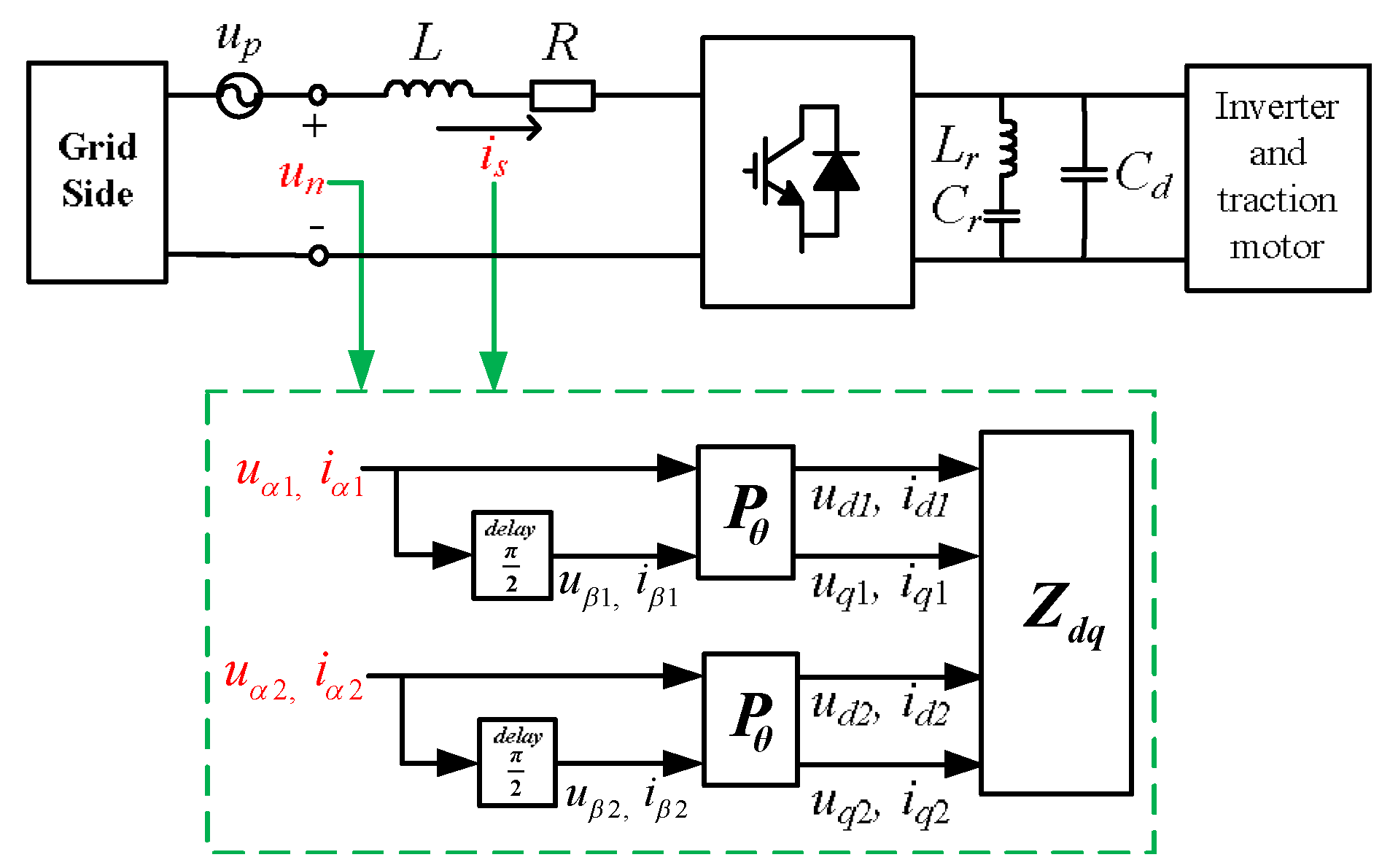
2.1. Input Impedance Model of Train

Traction converter is the main part of HSTs, which including grid-side converter, inverter and traction motor. Figure 1 shows the structure of a traction converter.

In Figure 1, the catenary voltage is 25 kV, and the second-side voltage of traction transformer is e_s. The leakage inductance and resistance of traction transformer are L and R, respectively. The grid-side current is i_s. The grid-side converter is a four-quadrant converter (4QC), which converts between AC and DC. The bridge arm voltage is u_ab. The switching components Q₁–Q₄ are four IGBTs (Insulated Gate Bipolar Transistor). The secondary resonant circuit is composed of inductance L_r and capacitor C_r. The DC side supporting capacitor is C_d, and the DC voltage is U_dc. Inverter and traction motor are connected on the DC side, which are the load of grid-side converter. According to Figure 1, the train model can be divided into two parts: a gird-side converter impedance model, and its load-inverter and a traction motor impedance model.

2.1.1. Impedance Model of the Grid-Side Converter

In order to make the grid-side converter impedance model more accurate, the modeling process is divided into several parts: Voltage Synchronization System (VSS), Current Synchronization System (CSS), AC Current Controller (ACC) and DC Voltage Controller (DVC). The whole control structure is shown in Figure 2.

In the following sections, the impedance models of VSS, CSS, ACC, and DVC are established in turns.

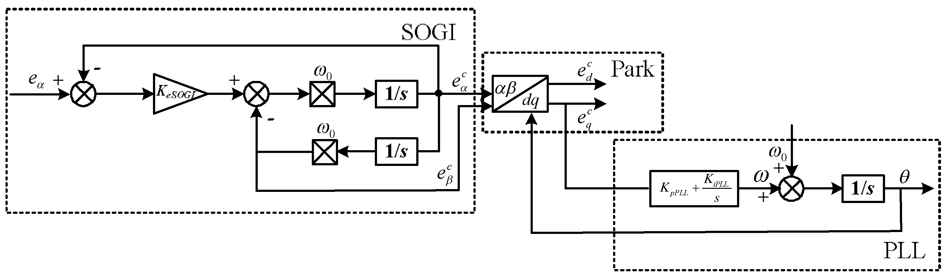
A. Model of Voltage Synchronization System (VSS)

The structure of VSS is shown in Figure 3 [11]:

In Figure 3, e is the transformer secondary side voltage. The superscript c represents the control quantity. The gain of SOGI is K_eSOGI. The angular frequency of the power frequency is ${\omega }_0$. The synchro angle generated by the phase-locked loop (PLL) is $\theta$. From the quantities introduced above, the following equation can be formed:

$$\underset{{\mathit{e}}_{\mathit{\alpha }\mathit{\beta }}^{\mathit{c}}}{\underbrace{\left[\begin{array}{l}{e}_{\alpha }^c\\ e_{\beta }^c\end{array}\right]}}=\underset{{\mathit{H}}_{\mathit{e}}}{\underbrace{\left[\begin{array}{ll}{H}_e& 0\\ 0& H_e\end{array}\right]}}\underset{{\mathit{e}}_{\mathit{\alpha }\mathit{\beta }}}{\underbrace{\left[\begin{array}{l}{e}_{\alpha }\\ e_{\beta }\end{array}\right]}}$$

(1)

$$H_e(s)=\frac{K_{eSOGI}{\omega }_{0}s}{s^2+K_{eSOGI}{\omega }_{0}s+{\omega }_0^2}$$

(2)

After Park transformation of ${\mathit{e}}_{\mathit{\alpha }\mathit{\beta }}^{\mathit{c}}$, ${\mathit{e}}_{\mathit{d}\mathit{q}}^{\mathit{c}}$ can be obtained [11]:

$${\mathit{e}}_{\mathit{d}\mathit{q}}^{\mathit{c}}={\mathit{P}}_{\mathit{\theta }}{\mathit{H}}_{\mathit{e}}{\mathit{P}}_{{\mathit{\theta }}_0}^{-1}{\mathit{e}}_{dq}\approx {\mathit{P}}_{\mathbf{\Delta }\mathit{\theta }}{\mathit{H}}_{\mathit{e}\mathit{d}\mathit{q}}{\mathit{e}}_{dq}$$

(3)

In Equation (3), ${\mathit{P}}_{\mathbf{\Delta }\mathit{\theta }}=\left[\begin{array}{ll}1& \Delta \theta \\ -\Delta \theta & 1\end{array}\right]$. Because $\Delta \theta$ is quite small, ${\mathit{H}}_{\mathit{e}\mathit{d}\mathit{q}}$ is equal to $P_{{\theta }_0}{H}_e{P}_{{\theta }_0}^{-1}$ [11]. The form of ${\mathit{H}}_{\mathit{e}\mathit{d}\mathit{q}}$ is as follows:

$${\mathit{H}}_{\mathit{e}\mathit{d}\mathit{q}}=\left[\begin{array}{ll}{H}_{edq}& 0\\ 0& H_{edq}\end{array}\right]$$

(4)

According to [15]:

$$H_{edq}=\frac{1}{\frac{1}{K_{eSOGI}}\cdot (\frac{1}{{\omega }_0}+\frac{T_0}{8})s+1}$$

(5)

From the Equations (3)–(5) and a small signal transformation, we can get:

$$\{\begin{array}{l}\Delta e_d^c=H_{edq}\Delta e_d+\Delta \theta H_{edq}{e}_{q0}\\ \Delta e_q^c=-H_{edq}{e}_{d0}\Delta \theta +H_{edq}\Delta e_q\end{array}$$

(6)

Because of PLL, the form of $\Delta \omega$ is as follows:

$$\Delta \omega =s\Delta \theta =(K_{pPLL}+\frac{K_{iPLL}}{s})\Delta e_q^c=K_{PLL}\Delta e_q^c$$

(7)

From Equations (6) and (7), the form of $\Delta \theta$ can be obtained:

$$\Delta \theta =\underset{{\mathit{G}}_{\mathit{P}\mathit{L}\mathit{L}}}{\underbrace{\frac{K_{PLL}{H}_{edq}}{s+e_{d0}{K}_{PLL}{H}_{edq}}}}\Delta e_q$$

(8)

Substituting (8) into (6), the relation between $\Delta e^c$ and $\Delta e$ is in Equation (9):

$$\underset{\mathbf{\Delta }{\mathit{e}}^{\mathit{c}}}{\underbrace{\left[\begin{array}{l}\Delta e_d^c\\ \Delta e_q^c\end{array}\right]}}=\underset{{\mathit{G}}_{\mathit{e}\mathit{V}\mathit{S}\mathit{S}}}{\underbrace{\left[\begin{array}{ll}{H}_{edq}& G_{PLL}{H}_{edq}{e}_{q0}\\ 0& H_{edq}-H_{edq}{e}_{d0}{G}_{PLL}\end{array}\right]}}\underset{\mathbf{\Delta }\mathit{e}}{\underbrace{\left[\begin{array}{l}\Delta e_d\\ \Delta e_q\end{array}\right]}}$$

(9)

B. Model of Current Synchronization System (CSS)

According to VSS, the equations of CSS can be obtained easily:

$${\mathit{i}}_{\mathit{d}\mathit{q}}^{\mathit{c}}\approx {\mathit{P}}_{\mathsf{\Delta }\mathit{\theta }}{\mathit{H}}_{\mathit{i}\mathit{d}\mathit{q}}{\mathit{i}}_{dq}$$

(10)

Combining (8) and (10):

$$\underset{\mathbf{\Delta }{\mathit{i}}^{\mathit{c}}}{\underbrace{\left[\begin{array}{l}\Delta i_d^c\\ \Delta i_q^c\end{array}\right]}}=\underset{{\mathit{H}}_{\mathit{i}\mathit{d}\mathit{q}}}{\underbrace{\left[\begin{array}{ll}{H}_{idq}& 0\\ 0& H_{idq}\end{array}\right]}}\underset{\mathbf{\Delta }\mathit{i}}{\underbrace{\left[\begin{array}{l}\Delta i_d\\ \Delta i_q\end{array}\right]}}-\underset{{\mathit{G}}_{\mathit{i}\mathit{C}\mathit{S}\mathit{S}}}{\underbrace{\left[\begin{array}{ll}0& -i_{q0}{H}_{idq}{G}_{PLL}\\ 0& i_{d0}{H}_{idq}{G}_{PLL}\end{array}\right]}}\underset{\mathbf{\Delta }\mathit{e}}{\underbrace{\left[\begin{array}{l}\Delta e_d\\ \Delta e_q\end{array}\right]}}$$

(11)

C. Model of AC Current Controller (ACC)

The structure of ACC is shown in Figure 4.

In Figure 4, the subscript ref represents a reference value. The grid-side current is i, and the bridge arm voltage in grid-side converter is v. The actual value of modulated wave in d-q axis is $v_d^c$ and $v_q^c$. The following matrix can be obtained through Figure 1:

$$\left[\begin{array}{l}{v}_d^c\\ v_q^c\end{array}\right]=\left[\begin{array}{l}{e}_d^c\\ e_q^c\end{array}\right]-\left[\begin{array}{ll}R+sL& -{\omega }_{0}L\\ {\omega }_{0}L& R+sL\end{array}\right]\left[\begin{array}{l}{i}_d^c\\ i_q^c\end{array}\right]$$

(12)

After current loop decoupling, the d-q reference value of modulation wave can be obtained:

$$\left[\begin{array}{l}{v}_{dref}^{}\\ v_{qref}^{}\end{array}\right]=\left[\begin{array}{l}{e}_d^c\\ e_q^c\end{array}\right]-K_{ACC}\left[\begin{array}{l}{i}_{dref}-i_d^c\\ i_{qref}-i_q^c\end{array}\right]-\left[\begin{array}{ll}0& -{\omega }_{0}L\\ {\omega }_{0}L& 0\end{array}\right]\left[\begin{array}{l}{i}_d^c\\ i_q^c\end{array}\right]$$

(13)

In this equation, $K_{ACC}=K_{ip}+\frac{K_{ii}}{s}$, which is the PI of current loop.

The d-q axis reference value of the modulated wave is delayed, and then, the actual value of modulated wave in d-q axis can be obtained:

$$\left[\begin{array}{l}{v}_d^c\\ v_q^c\end{array}\right]=G_d\left[\begin{array}{l}{v}_{dref}\\ v_{qref}\end{array}\right]$$

(14)

In Equation (14), $G_d=\frac{1}{T_{d}s+1}$, which is the delay part [16].

From Equations (12)–(14):

$$\mathbf{\Delta }{\mathit{i}}^{\mathit{c}}={\mathit{G}}_{\mathit{i}\mathit{d}\mathit{q}\mathit{r}\mathit{e}\mathit{f}}\mathbf{\Delta }{\mathit{i}}_{\mathit{r}\mathit{e}\mathit{f}}+{\mathit{G}}_{\mathit{e}\mathit{d}\mathit{q}}^{\mathit{c}}\mathbf{\Delta }{\mathit{e}}^{\mathit{c}}$$

(15)

where ${\mathit{G}}_{\mathit{i}\mathit{d}\mathit{q}\mathit{r}\mathit{e}\mathit{f}}$, $\Delta {\mathit{i}}_{\mathit{r}\mathit{e}\mathit{f}}$, and ${\mathit{G}}_{\mathit{e}\mathit{d}\mathit{q}}^{\mathit{c}}$ can be expressed as:

$$\{\begin{array}{l}{\mathit{G}}_{\mathit{i}\mathit{d}\mathit{q}\mathit{r}\mathit{e}\mathit{f}}={({\mathit{G}}_{\mathit{d}\mathit{q}}^{\mathit{c}})}^{-1}{G}_d{K}_{ACC}\\ \mathbf{\Delta }{\mathit{i}}_{\mathit{r}\mathit{e}\mathit{f}}=\left[\begin{array}{l}\Delta i_{dref}\\ \Delta i_{qref}\end{array}\right]\\ {\mathit{G}}_{\mathit{e}\mathit{d}\mathit{q}}^{\mathit{c}}={({\mathit{G}}_{\mathit{d}\mathit{q}}^{\mathit{c}})}^{-1}(1-G_d)\\ {\mathit{G}}_{\mathit{d}\mathit{q}}^{\mathit{c}}=\left[\begin{array}{ll}{G}_d{K}_{ACC}+R+sL& {\omega }_{0}L(G_d-1)\\ -{\omega }_{0}L(G_d-1)& G_d{K}_{ACC}+R+sL\end{array}\right]\end{array}$$

(16)

Combining (9), (11) and (15):

$$\mathsf{\Delta }\mathit{i}=\underset{{\mathit{G}}_{\mathit{i}}}{\underbrace{{({\mathit{H}}_{\mathit{i}\mathit{d}\mathit{q}})}^{-1}{\mathit{G}}_{\mathit{i}\mathit{d}\mathit{q}\mathit{r}\mathit{e}\mathit{f}}}}\mathsf{\Delta }{\mathit{i}}_{\mathit{r}\mathit{e}\mathit{f}}+\underset{{\mathit{G}}_{\mathit{e}}}{\underbrace{{({\mathit{H}}_{\mathit{i}\mathit{d}\mathit{q}})}^{-1}({\mathit{G}}_{\mathit{i}\mathit{C}\mathit{S}\mathit{S}}+{\mathit{G}}_{\mathit{e}\mathit{d}\mathit{q}}^{\mathit{c}}{\mathit{G}}_{\mathit{e}\mathit{V}\mathit{S}\mathit{S}})}}\mathsf{\Delta }\mathit{e}$$

(17)

The equation of $\Delta \mathit{i}$ is as follows:

$$\mathsf{\Delta }\mathit{i}={\mathit{G}}_{\mathit{i}}\mathsf{\Delta }{\mathit{i}}_{\mathit{r}\mathit{e}\mathit{f}}+{\mathit{G}}_{\mathit{e}}\mathsf{\Delta }\mathit{e}$$

(18)

D. Model of DC Voltage Controller (DVC)

The purpose of modeling voltage loop is to find the relation of $\Delta {\mathit{i}}_{\mathit{r}\mathit{e}\mathit{f}}$ and $\Delta \mathit{e}$. With PI control, the d-axis reference $i_{dref}$ in small signal form is in Equation (19):

$$\Delta i_{dref}=-K_{VCC}(s)\Delta v_{dc}$$

(19)

where $K_{VCC}(s)=K_{vp}+\frac{K_{vi}}{s}$ is the PI of voltage loop.

The instantaneous active and reactive powers flowing into 4QC are, respectively, given by [14]:

$$P=\mathrm{Re}\{\mathit{e}{\mathit{i}}^{*}\}=\underset{P_0}{\underbrace{e_0{i}_{d0}}}+\underset{\Delta P}{\underbrace{e_0\Delta i_d+\Delta e_d{i}_{d0}+\Delta e_q{i}_{q0}}}$$

(20)

$$Q=\mathrm{Im}\{\mathit{e}{\mathit{i}}^{*}\}=\underset{Q_0}{\underbrace{-e_0{i}_{q0}}}-\underset{\Delta Q}{\underbrace{e_0\Delta i_q-\Delta e_d{i}_{q0}+\Delta e_q{i}_{d0}}}$$

(21)

Set the total power P, and the load power of 4QC is P_L:

$$P-P_L=\frac{1}{2}{C}_{dc}\frac{d{v}_{dc}^2}{dt}\Rightarrow s{C}_{dc}{v}_{dc0}\Delta v_{dc}=\Delta P-\Delta P_L$$

(22)

where $\Delta P_L=\Delta v_{dc}{i}_L+v_{dc}\Delta i_L$, and $i_L=\frac{v_{dc}}{Z_L}$. Substituting $\Delta P$ in (20) into (22):

$$\Delta P_L=\Delta v_{dc}\frac{v_{dc0}}{Z_L}+v_{dc0}\frac{\Delta v_{dc}}{Z_L}=\frac{2v_{dc0}}{Z_L}\Delta v_{dc}$$

(23)

Combining (18), (20), (21) and (23), $\Delta v_{dc}$ can be calculated:

$$\Delta v_{dc}=\underset{{\mathit{M}}_{\mathit{d}}}{\underbrace{\frac{e_0{G}_{e(1,1)}+\frac{P_0}{e_0}}{s{C}_{dc}{v}_{dc0}+\frac{2v_{dc0}}{Z_L}+e_0{G}_{i(1,1)}{K}_{vcc}}}}\cdot \Delta e_d+\underset{{\mathit{M}}_{\mathit{q}}}{\underbrace{\frac{e_0{G}_{e(1,2)}-\frac{Q_0}{e_0}}{s{C}_{dc}{v}_{dc0}+\frac{2v_{dc0}}{Z_L}+e_0{G}_{i(1,1)}{K}_{vcc}}}}\cdot \Delta e_q$$

(24)

Substituting (24) into (19), and set $\Delta i_{qref}=0$, $\Delta {\mathit{i}}_{\mathit{r}\mathit{e}\mathit{f}}$ can be obtained:

$$\left[\begin{array}{l}\Delta i_{dref}\\ \Delta i_{qref}\end{array}\right]=\underset{{\mathit{G}}_{\mathit{r}\mathit{e}\mathit{f}}}{\underbrace{\left[\begin{array}{ll}-K_{vcc}{\mathit{M}}_{\mathit{d}}& -K_{vcc}{\mathit{M}}_{\mathit{q}}\\ 0& 0\end{array}\right]}}\left[\begin{array}{l}\Delta e_d\\ \Delta e_q\end{array}\right]$$

(25)

Combining (18) and (25), the admittance of train is as follows:

$${\mathit{Y}}_{\mathit{t}\mathit{r}\mathit{a}\mathit{i}\mathit{n}}={\mathit{G}}_{\mathit{i}}{\mathit{G}}_{\mathit{r}\mathit{e}\mathit{f}}+{\mathit{G}}_{\mathit{e}}$$

(26)

2.1.2. Impedance Model of Inverter and Traction Motor

Firstly, the equivalent circuit of inverter and traction motor is shown in Figure 5.

The state equation of the inverter in the d-q coordinate system is given by:

$$\frac{d}{dt}\left[\begin{array}{l}{i}_d\\ i_q\end{array}\right]=\frac{1}{L_m}\left[\begin{array}{l}{v}_d\\ v_q\end{array}\right]-\left[\begin{array}{ll}0& -{\omega }_e\\ {\omega }_e& 0\end{array}\right]\left[\begin{array}{l}{i}_d\\ i_q\end{array}\right]-\frac{R_m}{L_m}\left[\begin{array}{l}{i}_d\\ i_q\end{array}\right]$$

(27)

The small signal model is used for modeling inverter and the traction motor. The small signal equation on DC side is given by [19]:

$$\Delta i_L=D_d\Delta i_d+I_d\Delta d_d+D_q\Delta i_q+I_q\Delta d_q$$

(28)

In d-q axis, the duty ratios in steady state are D_d and D_q. The small signals of the duty ratio are $\Delta d_d$ and $\Delta d_q$. The stable currents are i_d and i_q. The small signals of currents are $\Delta i_d$ and $\Delta i_q$.

The equation of small signal in AC side is:

$$\{\begin{array}{l}\Delta d_d{v}_{dc}+D_d\Delta v_{dc}=\Delta i_d(s{L}_m+R_m)-{\omega }_e{L}_m\Delta i_q\\ \Delta d_q{v}_{dc}+D_q\Delta v_{dc}=\Delta i_q(s{L}_m+R_m)+{\omega }_e{L}_m\Delta i_d\end{array}$$

(29)

The next step is to get inverter open-loop input impedance, which is also the input impedance of inverter during stable operation. Set $\Delta d_d=\Delta d_q=0$ [19], and the following equations can be obtained:

$$\{\begin{array}{l}\Delta i_d=\frac{{\omega }_e{L}_m{D}_q+D_d(s{L}_m+R_m)}{{(s{L}_m+R_m)}^2+{\omega }_e^2{L}_m^2}\Delta v_{dc}\\ \Delta i_q=\frac{D_q(s{L}_m+R_m)-{\omega }_e{L}_m{D}_d}{{(s{L}_m+R_m)}^2+{\omega }_e^2{L}_m^2}\Delta v_{dc}\end{array}$$

(30)

Combining (28) and (30), the input impedance of inverter and traction motor is:

$$Z_L=\frac{\Delta v_{dc}}{\Delta i_L}=\frac{{(s{L}_m+R_m)}^2+{\omega }_e^2{L}_m^2}{(D_d^2+D_q^2)(s{L}_m+R_m)}$$

(31)

The input impedance model of train can be obtained by substituting (31) into (24). In order to make the whole calculation process more distinct, and distinguish the control variables and the actual variables more clearly, the structure of all calculations is shown in Figure 6:

Since there is no frequency limit in the model process of VSS, CSS, ACC, DVC and the load, this modeling method is applicable to the full frequency range.

2.2. Output Impedance Model of Traction Network

The main difficulty of traction network modeling is to model the d-q coupling impedance. Here the modeling process is shown in detail. According to the uniform transmission line theory, the voltage and current of terminal can be calculated:

$$\{\begin{array}{l}u=u_1\cosh (\gamma x)-Z_c{i}_1\sinh (\gamma x)\\ i=i_1\cosh (\gamma x)-\frac{u_1}{Z_c}\sinh (\gamma x)\end{array}$$

(32)

where $\gamma$ is the propagation constant. The characteristic impedance is Z_c. Both of them are complex numbers. The beginning voltage and current are u₁ and i₁.

The impedance model of network is shown in Figure 7 [20]:

In Figure 7, the substation is abbreviated as SS, and the section post is abbreviated as SP. The equivalent impedance of a substation is Z_ss. The equivalent impedance and admittance in left side and right side of the train are Z_T1, Y_T1 and Z_T2, Y_T2 respectively. The total length and impedance between SS and train are l₁ and Z₁. The total length and impedance between train and SP are l₂ and Z₂.

And the impedance of right-side of the train can be calculated:

$$\{\begin{array}{l}{Z}_{\mathrm{T}2}=\frac{Z_c[\cosh (\gamma l_2)-1]}{\sinh (\gamma l_2)}\\ Y_{\mathrm{T}2}=\frac{\sinh (\gamma l_2)}{Z_c}\end{array}$$

(33)

The next step is to make the model more concrete by showing every component, and calculate the coupling impedance of the network. The equivalent circuit of traction network diagram is shown in Figure 8:

In Figure 8, the resistance R₁ and inductance L₁ form the equivalent impedance Z_T1 in Figure 7. The capacitance C₁ and conductance G₁ form the equivalent admittance Y_T1. It is similar with the components in the right side of the train. Voltage u₁ and current i₁ are generated by train. Voltage u is the terminal port voltage.

Based on Kirchhoff’s theorem, voltage and current equation in right side of the circuit is given by:

$$i_1{R}_2+L_2\frac{d{i}_1}{dt}+i_1\frac{1}{G_2}+\frac{1}{C_2}{\displaystyle \int i_{1}dt=u_1}$$

(34)

Combining (32) and (34), and make it in s domain:

$$i_1{R}_2+i_1{L}_{2}s+u_1\cosh (\gamma l_2)-Z_c{i}_1\sinh (\gamma l_2)=u_1$$

(35)

The current i₁ and voltage u₁ can be written in d-q form:

$$\{\begin{array}{l}{i}_1=i_d\sin \omega t+i_q\cos \omega t\\ u_1=u_d\sin \omega t+u_q\cos \omega t\end{array}$$

(36)

Combining (35) and (36), and make the sine and cosine part in left side equal to sine and cosine part in right side respectively. The following matrix is obtained:

$$\left[\begin{array}{l}{u}_d\\ u_q\end{array}\right]=\left[\begin{array}{ll}\frac{R_2+s{L}_2-Z_c\sinh (\gamma l_2)}{1-\cosh (\gamma l_2)}& -\frac{L_2{\omega }_0}{1-\cosh (\gamma l_2)}\\ \frac{L_2{\omega }_0}{1-\cosh (\gamma l_2)}& \frac{R_2+s{L}_2-Z_c\sinh (\gamma l_2)}{1-\cosh (\gamma l_2)}\end{array}\right]\left[\begin{array}{l}{i}_d\\ i_q\end{array}\right]$$

(37)

where ${\omega }_0$ is the angular frequency of network.

What needs to be clear here is that R₂, G₂, C₂, L₂ are related to Z_T2 and Y_T2:

$$\{\begin{array}{l}{Z}_{\mathrm{T}2}=R_2+j\omega L_2=\frac{Z_c[\cosh (\gamma l_2)-1]}{\sinh (\gamma l_2)}\\ Y_{\mathrm{T}2}=G_2+j\omega C_2=\frac{\sinh (\gamma l_2)}{Z_c}\end{array}$$

(38)

The aforementioned $\gamma$ and Z_c are both complex numbers, so they can be expressed as:

$$\{\begin{array}{l}{Z}_c=\sqrt{\frac{Z_0}{Y_0}}=\sqrt{\frac{R_0+j\omega L_0}{G_0+j\omega C_0}}=m+jn\\ \gamma =\sqrt{Z_0{Y}_0}=\sqrt{(R_0+j\omega L_0)(G_0+j\omega C_0)}=\alpha +j\beta \end{array}$$

(39)

Combining (38) and (39), the R₂, G₂, C₂, L₂ can be obtained.

$$\{\begin{array}{l}{R}_2=\frac{1}{C^2+D^2}\cdot \{m[C(A-2)+BD]-n[BC-D(A-2)]\}\\ G_2=\frac{1}{2(m^2+n^2)}\cdot [m(e^{\alpha l_2}\cos \beta l_2-e^{-\alpha l_2}\cos \beta l_2)+n(e^{\alpha l_2}\sin \beta l_2+e^{-\alpha l_2}\sin \beta l_2)]\\ C_2=\frac{1}{2\omega (m^2+n^2)}\cdot [m(e^{\alpha l_2}\sin \beta l_2+e^{-\alpha l_2}\sin \beta l_2)-n(e^{\alpha l_2}\cos \beta l_2-e^{-\alpha l_2}\cos \beta l_2)]\\ L_2=\frac{1}{\omega (C^2+D^2)}\cdot \{m[BC-D(A-2)]+n[C(A-2)+BD]\}\end{array}$$

(40)

where:

$$\{\begin{array}{l}{e}^{\alpha l_2}\cos \beta l_2+e^{-\alpha l_2}\cos \beta l_2=A\\ e^{\alpha l_2}\sin \beta l_2-e^{-\alpha l_2}\sin \beta l_2=B\\ e^{\alpha l_2}\cos \beta l_2-e^{-\alpha l_2}\cos \beta l_2=C\\ e^{\alpha l_2}\sin \beta l_2+e^{-\alpha l_2}\sin \beta l_2=D\end{array}$$

(41)

Combining (37) and (40), the matrix of network impedance on right side of the train can be obtained, which is similar to the left side.

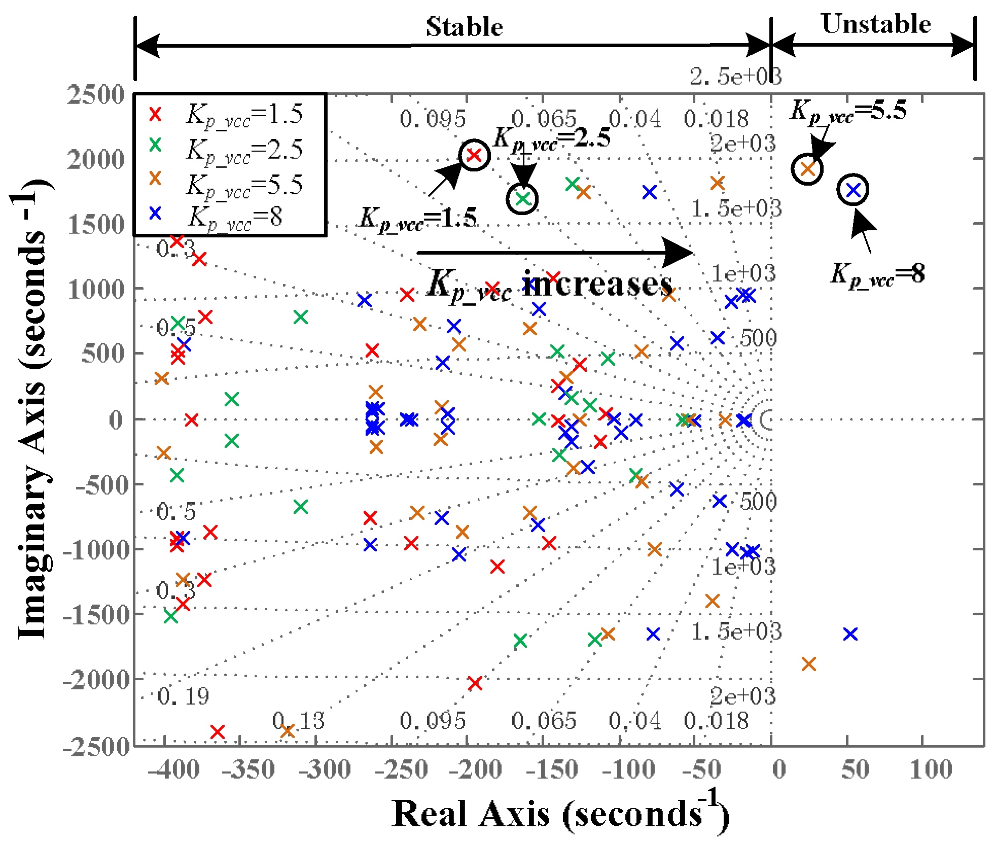
3. Stability Analysis of the Overall Power System

In the following part, the system stability will be analyzed in the full frequency domain using the impedance model proposed in this paper. First, the concept of total train-network input impedance is introduced to analyze the resonance frequency [21]. Figure 9 shows the coupling analysis model of the train-network system. There is usually more than one power unit in a high-speed train, so here the letter n represents the number of power units. The total train-network input impedance Z_intk is composed of $n-1$ power unit impedances $Z_{trk}/\left(n-1\right)$ and the network impedance Z_ingk in parallel.

First, calculate Z_intk, where k denotes the k-order harmonics:

$${\mathit{Z}}_{\mathit{i}\mathit{n}\mathit{t}\mathit{k}}=\frac{{\mathit{Z}}_{\mathit{i}\mathit{n}\mathit{g}\mathit{k}}\cdot \frac{{\mathit{Z}}_{\mathit{t}\mathit{r}\mathit{k}}}{n-1}}{{\mathit{Z}}_{\mathit{i}\mathit{n}\mathit{g}\mathit{k}}+\frac{{\mathit{Z}}_{\mathit{t}\mathit{r}\mathit{k}}}{n-1}}=\frac{{\mathit{Z}}_{\mathit{i}\mathit{n}\mathit{g}\mathit{k}}}{\mathit{I}+(n-1){\mathit{Y}}_{\mathit{t}\mathit{r}\mathit{k}}{\mathit{Z}}_{\mathit{i}\mathit{n}\mathit{g}\mathit{k}}}$$

(42)

According to Equation (42), the relationship between total train-network input impedance, frequency and the length of catenary can be obtained and shown in Figure 10:

It can be seen from the figure that the train-network input impedances of d-d, d-q, q-d and q-q axes are slightly different. This figure can reflect the oscillation frequency of the train-network with a certain frequency range, because the frequency corresponding to the peak of total train-network input impedance is the system parallel resonance frequency [21]. From the figure, it is also obvious that the input impedances of train-network of all axis still follow the rule—the greater the length of catenary, the lower the oscillation frequency [5], which means as the length of the catenary increases, the local train-network oscillation frequency shifts to the left on the frequency axis.

In the following part, we will analyze the system stability from another perspective—closed-loop transfer function. The train-network impedance model is simplified in Figure 11:

Here e_s and Z_s are the voltage and the output impedance of network on the secondary side of the traction transformer, respectively; the input current of the train is i_s, and the input impedance of the train is Z_tr.

In references [18] and [22], the equation of closed-loop transfer function of the system is given by:

$$\begin{array}{ll}{\mathit{H}}_{\mathit{s}}(\mathit{s})& =\frac{{\mathit{i}}_{\mathit{s}}(\mathit{s})}{{\mathit{e}}_{\mathit{s}}(\mathit{s})}=\frac{1}{{\mathit{Z}}_{\mathit{s}}(\mathit{s})+\frac{{\mathit{Z}}_{\mathit{t}\mathit{r}}(\mathit{s})}{n}}\\ & =\frac{n{\mathit{Y}}_{\mathit{t}\mathit{r}}(\mathit{s})}{\mathit{I}+n{\mathit{Y}}_{\mathit{t}\mathit{r}}(\mathit{s})\cdot {\mathit{Z}}_{\mathit{s}}(\mathit{s})}\end{array}$$

(43)

where n is the number of converters. The pole figure of the closed-loop transfer function is used to determine the stability of the system by observing whether there is any pole in the right half-plane. The closed-loop transfer function in the form of matrix also has poles. Known from the Smith-Mcmillan Form, the pole of a matrix G(s) is the roots of the denominator in diagonal of M(s), which is the standard form of Smith-Mcmillan Form [23]. Therefore, the pole figure of the closed-loop transfer function could be obtained.

Figure 12 shows the pole figure of the closed-loop system while the parameter K_{p_vcc} increases. Different colors of poles indicate different K_{p_vcc} values in Y_tr(s). When K_{p_vcc} = 1.5 and 2.5, the poles are all in left half-plane, which means the system is stable. With K_{p_vcc} increasing, the poles of the system shift to the right plane. When K_{p_vcc} = 5.5 and 8, there are poles in right half-plane, which means the system become unstable. This figure shows that with K_{p_vcc} increasing, the system becomes unstable gradually.

4. Simulation and Experiment Result

4.1. Setup of Simulation and Experiment

In order to compare the train impedance model established in this paper with that of existing papers, and verify the proposed model, the following simulations are performed. And in order to verify the characteristic of this model in some degree, the experiment is performed. The parameters of simulation and experiment are shown in

Table 1. Simulation and experiment parameters.

Symbols	Note	Simulation Value	Experiment Value
ed0	d-channel steady state voltage	2000 V	2100 V
eq0	q-channel steady state voltage	0 V	0 V
P0	Active power	360 kW	360 kW
Q0	Reactive power	0 kW	0 kW
L	Leakage inductance of transformer	2.8 mH	2.8 mH
R	Leakage resistance of transformer	0.2 Ω	0.35 Ω
Td	Time delay	1.2 μs	1.2 μs
Kp_acc	Current loop proportional gain	3	4.5
Ki_acc	Current loop integral gain	0.8	0.8
Kp_vcc	Voltage loop proportional gain	1.5	1.5
Ki_vcc	Voltage loop integral gain	1.4	1.5
Kp_PLL	PLL-Proportional gain	5.5	6
Ki_PLL	PLL-Integral gain	97	50
KeSOGI	SOGI-voltage gain	0.8	0.8
KiSOGI	SOGI-current gain	1	1
Cdc	Capacitance in DC side	16 mF	16 mF
vdc0	DC voltage	1500 V	1500 V
Lm	Inductance of motor	43.8 mH	43.8 mH
Rm	Resistance of motor	0.223 Ω	0.223 Ω
we	Rotating speed	1000 rad/s	1000 rad/s
n	n modules	2	2
R0	Unit length residence of network	1.33 mΩ/km	-
L0	Unit length inductance of network	0.21 mH/km	-
G0	Unit length conductance of network	2 S/km	-
C0	Unit length capacitance of network	0.35 mF/km	-
l	Length of catenary	15 km	-

.

4.2. Simulation and Experiment Analysis

In this part, the calculated model proposed in this paper will be verified first. Referring to [11,24,25], the impedance measuring method for single-phase systems is used here, which is shown in Figure 13. In this figure, u_p is the perturbation injection. The voltage u_n and current i_s are regarded as the components in the $\alpha$ axis. At the very beginning of the verification experiment, the simulated grid-side converter will be operating in a steady state, and then u_p is added in this circuit. The voltage and current in d-q axis can be calculated, and the Z_dq can be obtained. The measured admittances are shown in Figure 14.

Figure 14 is the Bode diagram of train admittance in the d-d, d-q, q-d and q-q axes. Four conditions are shown in this figure. They are with SOGI and load model (proposed in this paper), with SOGI but without load model, without both SOGI and load model, and measured admittance. This figure shows that the measured admittance is consistence with the blue line (the model proposed in this paper). There are only some slight deviations in high-frequency. The calculated load model should be study further to make it more precise. It can also be seen from the figure that SOGI mainly affects the high-frequency part of d-d, q-d and q-q axes admittance, but has little effect on d-q axes admittance. The load model mainly affects the high-frequency part of d-d, q-d and q-q admittance. It has a certain influence on the full frequency band of d-q axis admittance.

Figure 12 shows that the increasing of K_{p_vcc} makes the system unstable. In the following part, this conclusion will be verified by simulation and experiment. First, establish a train-network united simulation and measure the grid-side voltage e_s, grid-side current i_s1 and i_s2, which are shown in Figure 15.

Figure 15 shows the simulation results about the influence of k_{p_vcc} increasing on grid-side voltage e_s and grid-side currents i_s1 and i_s2. In this figure, before 0.7 s the control parameter of 4QC voltage loop k_{p_vcc} takes the value of 1.5, and the system remains stable. At 0.7 s, k_{p_vcc} is changed to 5.5, and the grid-side voltage e_s starts to oscillate, and the grid-side currents i_s1 and i_s2 also begin to oscillate sharply and appear divergent. So this model can reflect the impact of parameters on the system stability. The next step is to verify whether this change is correct by experiment.

In order to simulate the actual 25 kV traction network in the laboratory, the two phases of the three-phase 380 V AC are taken and converted to 25 kV via a step-up transformer to supply the entire system. In order to make the grid-side converter (GC) work under load, it powers two inverters (INV) and the traction motors work in drag mode. The simplified schematic diagram of experimental operation is shown in Figure 16. It should be noted that there are two traction converters put into use, so the value of DC capacitor is doubled, which helps to reduce harmonics generated by two inverters. In addition, there is a LC resonance circuit in DC side, which reduces the 2nd order harmonic effectively, and the 2nd order is the main content in DC side if there is no such LC resonance circuit. Due to the reasons above, we ignore the interactions of the two inverters.

The experimental platform is shown in Figure 17. There are two IGBT modules in one grid-side converter, so it contains eight IGBTs. There is only one IGBT module in one inverter, which includes nine IGBTs. All these IGBT modules are in the back of one traction converter. All control parts (including grid-side converter controller, inverter controllers) are in the front of one traction converter. It should be noted that there are two inverters used in this experiment, so there are two traction converters paralleled in DC side. In one traction converter, both grid-side converter and inverter are put into use, and in the other one, only the inverter is put into use. There are two pairs of traction motors in drag mode.

Figure 18 is the experimental waveform. The grid-side voltage is e_s, the grid-side currents are i_s1 and i_s2, and U_dc is DC voltage. At the point of A, k_{p_vcc} increased from 1.5 to 5.5. As can be seen from this figure, the system cannot be stable again from the point of A, and the current waveforms are also divergent, which triggered the protection of the system. It should be noted that the grid-side voltage e_s in the experiment is a signal introduced from the primary side of the traction transformer directly. When the oscillation occurs, the grid-side voltage changes slightly, so after protection and when the system stops working, e_s can still become normal. Through experiments it is shown that the increase of the voltage loop parameter k_{p_vcc} does make the system unstable, which is consistent with the simulation. It further verifies the correct characteristic of the model described in this paper.

5. Conclusions

Firstly, an impedance model of a train in the d-q coordinate system is established in this paper. The proposed model is capable of reflecting the control scheme of the grid-side converter in details, which benefits the analysis of the impact of parameter changes on the system. The equivalent load models of grid-side converter are also taken into consideration, making the model more complete. The load model mainly affects the high-frequency part of d-d, q-d and q-q train admittance. It has a certain influence on the full frequency band of d-q axis train admittance. The load model cannot be ignored because of this influence. Secondly, this paper considers the impedance and admittance components of the network in the d-q coordinate system in more details, making the whole model more accurate. Thirdly, this model can help to analyze the stability of the whole system as seen in 3D figure and zero-pole diagram. Finally, from the results of simulation and experiment, this model can reflect the impact of parameter changes on the train-network system correctly.

In future research, the impedance models of inverter and traction motor also need further study. At present, only a simple d-q axis impedance model is established in this paper, and the control components of inverter and traction motor need to be considered later to create a more accurate load model. In addition, the influence of the equivalent coupling impedance (d-q and q-d axis impedance) of the train-network on the system needs further research.

References

1. Liu, Z.; Zhang, G.; Liao, Y. Stability research of high-speed railway EMUs and traction network cascade system considering impedance matching. IEEE Trans. Ind. Appl. 2016, 52, 4315–4326. [Google Scholar] [CrossRef]
2. Cui, H.; Song, W.; Ge, X.; Feng, X. High-frequency resonance suppression of high-speed railways in China. IET Electr. Syst. Transp. 2016, 6, 88–95. [Google Scholar] [CrossRef]
3. Rocabert, J.; Luna, A.; Blaabjerg, F.; Rodriguez, P. Control of power converters in AC microgrids. IEEE Trans. Power Electron. 2012, 27, 4734–4749. [Google Scholar] [CrossRef]
4. Harnefors, L.; Yepes, A.G.; Vidal, A.; Doval-Gandoy, J. Passivity-based controller design of grid-connected VSCs for prevention of electrical resonance instability. IEEE Trans. Ind. Electron. 2015, 62, 702–710. [Google Scholar] [CrossRef]
5. Hu, H.; Tao, H.; Wang, X.; Blaabjerg, F.; He, Z.; Gao, S. Train–Network Interactions and Stability Evaluation in High-Speed Railways—Part II: Influential Factors and Verifications. IEEE Trans. Power Electron. 2018, 33, 4643–4659. [Google Scholar] [CrossRef]
6. Mollerstedt, E.; Bernhardsson, B. Out of control because of harmonics—An analysis of the harmonic response of an inverter locomotive. IEEE Control Syst. 2000, 20, 70–81. [Google Scholar] [CrossRef]
7. Hu, H.; Shao, Y.; Tang, L.; Ma, J.; He, Z.; Gao, S. Overview of harmonic and resonance in railway electrification systems. IEEE Trans. Ind. Appl. 2018. [Google Scholar] [CrossRef]
8. Zhang, G.; Liu, Z.; Yao, S.; Liao, Y.; Xiao, C. Suppression of low-frequency oscillation in traction network of high-speed railway based on auto-disturbance rejection control. IEEE Trans. Transp. Electr. 2016, 2, 244–255. [Google Scholar] [CrossRef]
9. Liu, Z.; Zhang, G.; Liao, Y. The stability research of high-speed railway EMUs and traction network cascade system. In Proceedings of the Electrical Machines & Power Electronics (ACEMP), Side, Turkey, 2–4 September 2015; pp. 123–128. [Google Scholar]
10. Cui, H.; Feng, X.; Song, W. High-Order Harmonic Load Modeling Method for High-Speed Railway. Electr. Power Autom. Equip. 2013, 33, 92–99. (In Chinese) [Google Scholar]
11. Wang, H.; Wu, M.; Sun, J. Analysis of low-frequency oscillation in electric railways based on small-signal modeling of vehicle-grid system in dq frame. IEEE Trans. Power Electron. 2015, 30, 5318–5330. [Google Scholar] [CrossRef]
12. Liao, Y.; Liu, Z.; Zhang, G.; Xiang, C. Vehicle-grid system stability analysis considering impedance specification based on norm criterion. In Proceedings of the Transportation Electrification Asia-Pacific (ITEC Asia-Pacific), Busan, Korea, 1–4 June 2016; pp. 118–123. [Google Scholar]
13. Wen, B.; Boroyevich, D.; Burgos, R.; Mattavelli, P.; Shen, Z. Analysis of DQ small-signal impedance of grid-tied inverters. IEEE Trans. Power Electron. 2016, 31, 675–687. [Google Scholar] [CrossRef]
14. Harnefors, L.; Bongiorno, M.; Lundberg, S. Input-admittance calculation and shaping for controlled voltage-source converters. IEEE Trans. Ind. Electron. 2007, 54, 3323–3334. [Google Scholar] [CrossRef]
15. Danielsen, S.; Fosso, O.B.; Molinas, M.; Suul, J.A.; Toftevaag, T. Simplified models of a single-phase power electronic inverter for railway power system stability analysis—Development and evaluation. Electr. Power Syst. Res. 2010, 80, 204–214. [Google Scholar] [CrossRef]
16. Hu, H.; Tao, H.; Blaabjerg, F.; Wang, X.; He, Z.; Gao, S. Train–Network Interactions and Stability Evaluation in High-Speed Railways—Part I: Phenomena and Modeling. IEEE Trans. Power Electron. 2018, 33, 4627–4642. [Google Scholar] [CrossRef]
17. Zhang, C.; Wang, X.; Blaabjerg, F. Analysis of phase-locked loop influence on the stability of single-phase grid-connected inverter. In Proceedings of the Power Electronics for Distributed Generation Systems (PEDG), Aachen, Germany, 22–25 June 2015; pp. 1–8. [Google Scholar]
18. Tao, H.; Hu, H.; Wang, X.; Blaabjerg, F.; He, Z. Impedance-Based Harmonic Instability Assessment in Multiple Electric Trains and Traction Network Interaction System. IEEE Trans. Ind. Appl. 2018. [Google Scholar] [CrossRef]
19. Wen, W. Dynamic Characteristic and Control of Power Electronic Cascade Systems. Power Convers. 2006, 28, 13–16. (In Chinese) [Google Scholar]
20. Hu, H.; Zhang, M.; Qian, C.; He, Z.; Fang, L. Research on the harmonic transmission characteristic and the harmonic amplification and suppression in high-speed traction system. In Proceedings of the Power and Energy Engineering Conference (APPEEC), Wuhan, China, 25–28 March 2011; pp. 1–4. [Google Scholar]
21. Cui, H.; Song, W.; Fang, H.; Ge, X.; Feng, X. Resonant harmonic elimination pulse width modulation-based high-frequency resonance suppression of high-speed railways. IEEE Trans. Power Electron. 2015, 8, 735–742. [Google Scholar] [CrossRef]
22. Liao, Y.; Liu, Z.; Zhang, G.; Xiang, C. Vehicle-Grid System Modeling and Stability Analysis with Forbidden Region-Based Criterion. IEEE Trans. Power Electron. 2017, 32, 3499–3512. [Google Scholar] [CrossRef]
23. Hosoe, S. On a time-domain characterization of the numerator polynomials of the Smith McMillan form. IEEE Trans. Autom. Control 1975, 20, 799–800. [Google Scholar] [CrossRef]
24. Liao, Y.; Liu, Z.; Zhang, H.; Wen, B. Low-Frequency Stability Analysis of Single-Phase System with dq-Frame Impedance Approach—Part II: Stability and Frequency Analysis. IEEE Trans. Ind. Appl. 2018. [Google Scholar] [CrossRef]
25. Liao, Y.; Liu, Z.; Hu, X.; Wen, B. A dq-Frame Impedance Measurement Method based on Hilbert Transform for Single-Phase Vehicle-Grid System. In Proceedings of the Transportation Electrification Asia-Pacific (ITEC Asia-Pacific), Harbin, China, 7–10 August 2017; pp. 1–6. [Google Scholar]
Figure 1. Structure figure of a traction converter.
Energies 11 01714 g001
Figure 2. Controller of network-side converter.
Energies 11 01714 g002
Figure 3. The structure of VSS.
Energies 11 01714 g003
Figure 4. The structure of ACC.
Energies 11 01714 g004
Figure 5. Equivalent circuit of inverter and traction motor.
Energies 11 01714 g005
Figure 6. The structure of all calculations.
Energies 11 01714 g006
Figure 7. Impedance model of traction network.
Energies 11 01714 g007
Figure 8. Equivalent circuit of traction network.
Energies 11 01714 g008
Figure 9. Train-network system coupling analysis model.
Energies 11 01714 g009
Figure 10. Relationship between total train-network input impedance, frequency and the length of catenary.
Energies 11 01714 g010
Figure 11. Simplified model of train-network.
Energies 11 01714 g011
Figure 12. Pole figure of train-network.
Energies 11 01714 g012
Figure 13. The impedance measuring method model.
Energies 11 01714 g013
Figure 14. Admittance Bode figure of train.
Energies 11 01714 g014
Figure 15. Simulation results about the influence of kp_vcc increasing on the system.
Energies 11 01714 g015
Figure 16. Simplified schematic diagram of experimental operation.
Energies 11 01714 g016
Figure 17. Experimental platform of the whole system.
Energies 11 01714 g017
Figure 18. Experimental figure about kp_vcc change.
Energies 11 01714 g018