Article

Power System Day-Ahead Unit Commitment Based on Chance-Constrained Dependent Chance Goal Programming

1
State Key Laboratory of Alternate Electrical Power System with Renewable Energy Sources, North China Electric Power University, Baoding 071003, China
2
Dispatching and Control Center of State Grid Qinghai Electric Power Company, Xining 810008, China
*
Authors to whom correspondence should be addressed.
Energies 2018, 11(7), 1718; https://doi.org/10.3390/en11071718
Submission received: 15 May 2018 / Revised: 8 June 2018 / Accepted: 18 June 2018 / Published: 1 July 2018

Abstract

:
In the context of large-scale renewable energy integrated into an electrical power system, the effects of power forecast errors on the power balance equation of the power system unit commitment model is considered. In this paper, the problem of solving the power balance equation with uncertain variables was studied. The unit commitment model with random variables in the power balance equation was solved by establishing a power system day-ahead optimisation unit commitment model based on chance-constrained dependent chance goal programming. First, to achieve the solution of the power balance equation with random variables, the equality constraint is loosened into an inequality constraint, and the power balance equation constraint is transformed into a dependent chance programming model aimed at maximising the probability of occurrence of random events in an uncertain environment. Then, the dependent chance programming model is proposed to ensure the economy and security of the scheme, and the goal programming model is introduced to facilitate an efficient solution. By combining dependent chance programming and goal programming, a power system day-ahead unit commitment model based on chance-constrained dependent chance goal programming is established. Finally, an example is discussed to demonstrate the effectiveness of the proposed model.

1. Introduction

The unit commitment (UC) problem is defined as an optimization problem which determines the operating schedule of a set of generating units at each time interval with varying loads and generations, considering a set of operational, technical, economic, and environmental constraints [1,2]. With increasing concerns about climate change and fossil energy depletion, the power system has seen a fast expansion of renewable energy (RE) in recent years. Unlike conventional generating units, the power of RE, like wind and solar, cannot be predicted with perfect accuracy [3,4,5], which increases variability and uncertainty when integrating into the power system. Reference [6] presented a review dealing with the impacts that significant penetration of RE has on the UC models. Due to the uncertainty of RE, the reserve decision is largely considered as a severe problem in UC. It is a challenge to economically optimize reserve capacity, because a small change of reserve capacity may initiate a new generator and thus significantly raise operational costs [7,8,9]. Besides the traditional power system spinning reserve, various kinds of reserve such as demand response (DR), battery energy storage, and electric vehicles (EV) have been widely used to provide reserve for wind power [8,10,11,12]. Reference [11] establishes an effective UC model by optimizing reserves, and reference [13] proposes a multi-timing scheduling concept to optimize reserves. Aiming to achieve better computational efficiency and economy of the UC solutions, reference [14] proposes a new network-constrained UC approach by introducing newly proposed reserve models and simplified network constraints.
With the increasing proportion of RE integrated in the power system, considering it as a deterministic constant in the UC model can no longer meet the requirements of safe, reliable, cost-effective operation of the system [14,15,16]. The uncertainty of wind power is reflected in the uncertainty of nodal power injection, which is mainly caused by output forecast error [17,18]. Although several deterministic and stochastic ways [5] have been proposed to predict wind power output, the forecast error is still inevitable. This forecast error is usually represented by uncertain variables in the UC model. Therefore, it is necessary to study the optimal UC model with uncertain variables after the large-scale integration into the power system with wind power and photovoltaic power.
Generally, the UC models with uncertain variables are mainly robust UC [19,20,21], interval UC [22,23], and stochastic UC [24,25,26,27,28,29]. In the deterministic UC (DUC) model, the net load is the only uncertain variable, and is handled using reserve capacity [13]. Based on the traditional UC model, the different processing strategies for this uncertain variable form a variety of uncertain optimal UC models today; robust UC (RUC) considers the influence of uncertain variables in the objective function, and searches for the optimal power generation scheme under the worst conditions of uncertain variables [10,19]. However, the results are relatively conservative and usually make the costs high [20]. To deal with this, budget constraints are often used in RUC to mitigate its over-conservatism [19,21]. As with RUC, the interval UC (IUC) considers the possible wind power output within the given bounds, and the probabilistic distribution information is ignored. IUC considers uncertainties with transitions from upper to lower bounds between any two consecutive time periods, so it avoids identifying the worst conditions of uncertain variables, and the solution is faster than the RUC [22]. Like RUC, IUC is often too conservative and uneconomical. In order to deal with this, relaxing the ramping constraints was proposed in reference [23] to reduce the conservativeness of IUC. Chance-constrained programming (CCP) models consider the influence of uncertain variables in partial constraints which can be violated with a predefined probability level [24]. Considering load and wind uncertainties in the UC problem, the system spinning reserve capacity or line transmission capacity constraints affected by load and wind uncertainties are often set as the chance constraints [25,26,27]. Considering the uncertainty of forecast error and requirement of reserve decision, chance-constrained programming is regarded as a suitable method to establish a novel UC model in this paper. The scenario based stochastic UC (SUC) addresses uncertainties in both objective function and constraints [28,29], which generates multiple deterministic scenarios based on the distribution of uncertain variables, and then uses the generated multiple scenarios representing uncertain variables in the UC modelling and the solution [30,31,32]. Even with advanced scenario reduction techniques, multiple scenarios increase computational complexities and model solution time, which prevents large-scale SUC application [30,33]. In addition, reduced scenarios inevitably discard some stochastic characteristics information of wind power, especially when the adopted scenarios are very few [20]. Considering the time-varying feature of forecast error and requirement decision, Value-at-Risk (VaR) or Conditional VaR (CVaR) are also applied to model risks associated with the decisions in a stochastic environment [34,35]. Some hybrid UC models (HUC) are also proposed, which combine some of the approaches above [36,37].
Existing uncertain optimal UC models mainly focus on the effects of uncertain variables on the objective function [10,19,30], reserve capacity [25,26,27], and line or transmission section power [27] without considering the influence of uncertain variables on the power balance equation. In the case of small-scale wind power, the deviation of source and load power caused by the forecast error is small, and the effects on the safety and economic efficiency of power system operation is also small; however, with the increasing scale of wind power, its effects on the safe and economic operation of the power system cannot be ignored [38,39]. To absorb more wind power, the impact of wind power forecast error on the UC model power balance equation should be accurately researched to reduce the unbalance of electric power supply and demands caused by wind power uncertainty.
Based on this, this paper no longer ignores the forecast error in the power balance equation of the UC model, and proposes a power system day-ahead UC model based on chance-constrained dependent chance goal programming. In this model, in order to solve the power balance equation with uncertain variables, the equality constraint is loosened into an inequality constraint under uncertain sets, and then the dependent chance programming model is established to be put into the goal programming model with the highest priority for solution. Compared with existing work, the main contributions of the paper are as follows.
(1)
Wind power and load forecast error is considered to describe an accurate power balance equation to reduce the impact of wind power and load uncertainty. In order to solve the equation containing uncertain variables, the author put forward a model based on the dependent chance programming. To the authors’ knowledge, this is the first time someone has used dependent chance programming to deal the power balance equation in UC models. The novel model improves not only operation efficiency and wind power consumption, but also the level of power balance of the UC result after considering the forecast error.
(2)
Methodologically, we put forward the chance-constrained dependent chance goal programming and apply it to the day-ahead UC problem. According to the probability density function (PDF) of the forecast error, a reserve decision method is proposed based on chance-constrained programming (CCP) to efficiently utilize the reserve. In order to solve the multi-objective programming model rapidly, goal programming (GP) is introduced. Combined with the dependent chance programming used for solving the power balance equation containing uncertain variables, we propose chance-constrained dependent chance goal programming and apply it to the day-ahead UC problem, which introduces a novel method to deal with the uncertainties in the UC.
(3)
Mathematically, the stochastic problem is converted into a deterministic equivalent by mathematical derivation. Based on that, the model is transformed into a mixed integer quadratic programming (MIQP) problem, which provides an efficient solution.
The rest of the paper is organised as follows: the power balance equation in a day-ahead UC model of a power system is proposed in Section 2; Section 3 gives the power system day-ahead UC based on chance-constrained dependent chance goal programming; a model solution is presented in Section 4, and a case study is presented in Section 5; discussion is introduced in Section 6, and key conclusions are drawn in Section 7.

2. Power Balance Equation in a Day-Ahead UC Model of a Power System

2.1. Uncertain Variables in the Power Balance Equation

To maintain the safety and stability of the operating power system, it is necessary to maintain a balance between the power generation and the total load power in the system. For this reason, power balance constraints need to be met when formulating a day-ahead UC of a power system. The power generated by all generators is equal to the total system load and loss. Due to the UC scheme needing to be made before observing the uncertain power supply and the actual power of the load, it is necessary to use various forecasting techniques to predict the output of the uncertain power supply of load in advance. Not only do wind speed, wind direction, temperature, turbine type, turbine position, terrain roughness, air density, and wake effect [40,41] combine to make it difficult to predict the output, but, at the same time, due to factors such as temperature, human social activities, and consumption behaviours [42,43,44], there are inevitable errors in load forecasts. The forecast error of load and an Elia-Connected wind power generator in Belgium in 2016 are shown in Figure 1.
In Figure 1, it can be seen that forecast errors are unavoidable for wind power and load day-ahead forecasting. In the power system UC model, the actual wind power output and load are usually represented by the sum of the determined forecast value and the uncertain forecast error. Until the actual wind power and load output are observed, forecast errors are always uncertain variables, and are denoted by ε i . t w and ε t l o a d , respectively.

2.2. Treatment of the Power Balance Equation with Uncertain Variables

In order to ensure the frequency stability in the power system, the generated power and the consumed power need to be balanced at all times. Therefore, when formulating a UC plan, it is necessary to ensure that the power generated by all power supplies is equal to the sum of the power consumed by the load and the loss of the power grid [45]. The strict power balance equation considering forecast errors of wind power and load is [46]:
i = 1 N g P i . t + i = 1 N w ( P i . t w + ε i . t w Δ P i . t w ) = P t l o a d + ε t l o a d Δ P t l o a d + P t l o s s
where P i . t is the power of the thermal unit i at time t; P i . t w is the predicted power of the wind farm i at time t; ε i . t w is the power forecast error of the wind farm i at time t; Δ P i . t w is the power curtailment of wind farm i at time t when making a UC scheme; P t l o a d is the predicted power of system load at time t; ε t l o a d represents the load forecast error at time t; Δ P t l o a d is the possible lost load when making a UC scheme; and P t l o s s denotes the system network loss at time t.
The existing power system day-ahead UC model, deterministic UC model, chance-constrained stochastic UC model, robust UC, and interval optimal UC model all directly ignore ε i . t w and ε t l o a d in the power balance (Equation (1)) and convert it to Equation (2). The scenario method involves balancing each of the possible scenarios of uncertain variables as in Equation (3). Elsewhere [1], it is proposed that the stochastic variables in the power balance equation are replaced by their expected values based on the consideration of the minimum amount of conventional unit adjustment caused by the forecast errors, as given by Equation (4).
i = 1 N g P i . t + i = 1 N w ( P i . t w Δ P i . t w ) = P t l o a d Δ P t l o a d + P loss . t
i = 1 N g P i . s . t + i = 1 N w ( P i . t w + ε i . s . t w Δ P i . s . t w ) = P t l o a d + ε s . t l o a d Δ P s . t l o a d + P s . t l o s s
i = 1 N g P i . t + i = 1 N w ( P i . t w + E ( ε i . t w ) Δ P i . t w ) = P t l o a d + E ( ε t l o a d ) Δ P t l o a d + P t l o s s
where P i . s . t , ε i . s . t w , Δ P i . s . t w , ε s . t l o a d , Δ P s . t l o a d , and P s . t l o s s represent the thermal units generation power, wind power forecast error, wind power curtailment, load forecast error, load loss power, and system network loss in the error scenario s, respectively; E ( ε i . t w ) and E ( ε t l o a d ) represent the expected wind power and load forecast error, respectively.
The strict power balance equation (Equation (1)) considers forecast errors and contains both stochastic and deterministic variables, so it cannot be directly solved to obtain a deterministic UC scheme. In addition, the power balance model represented by Equations (2) to (4) with only deterministic variables and constants can be directly put into the UC model to obtain a deterministic UC scheme. However, the treatment of Equation (2) is simple but inaccurate and it is acceptable when only uncertain variables of the load forecast errors are involved. With the increasing scale of renewable energy, the variation range and effects of uncertain variables that represent the forecast error of renewable energy will become larger. The treatment of Equation (4) is reasonable to some extent, especially in the case in which the forecast error mean is not zero, then it is beneficial to the adjustment of the unit output scheme, however, it cannot cope with the challenges brought about by the increase in the uncertainty of the error caused by the increasing scale of renewable energy output. The processing method of Equation (3) is only applicable to the stochastic UC model based on the scenario method, and the power supply and load are balanced separately in a few reserved scenarios. The core idea of the scenario method is to use a large number of deterministic scenarios to represent the possible values of uncertain variables. Various scenario reduction techniques that increase the speed of calculation inevitably lead to the loss of uncertain variable information.
To solve Equation (1), containing both stochastic and deterministic variables, a new processing method was proposed: first, Equation (1) will be loosened to an inequality constraint to construct a set under an uncertain environment, as shown by Equation (5):
| i = 1 N g P i . t + i = 1 N w ( P i . t w + ε i . t w Δ P i . t w ) ( P t l o a d + ε t l o a d Δ P t l o a d + P t l o s s ) | σ
where σ is a small, deterministic constant that represents the range of the feasible set under an uncertain environment. When σ = 0, Equation (5) degenerates to Equation (1). Under the definition of Equation (5), the power balance (Equation (1)) is transformed into the probability of maximising the set in an uncertain environment, as per Equation (6):
max   Pr { | i = 1 N g P i . t + i = 1 N w ( P i . t w + ε i . t w Δ P i . t w ) ( P t l o a d + ε t l o a d Δ P t l o a d + P t l o s s ) | σ t }
The meaning of this equation can be illustrated by Figure 2.
The left-hand part of Figure 2 is a thermodynamic diagram of 10,000 actual power scenarios of wind power generation, corresponding to P i . t w + ε i . t w in Equation (5), while the right-hand part is the thermodynamic diagram of 10,000 actual power scenarios of load, corresponding to P t l o a d + ε t l o a d in Equation (5). The optimisation process enshrined in Equation (6) aims to adjust the deterministic output of the thermal units so that the total power output including wind power is most likely to match the load power. Compared with the power balance equation (Equation (2)) that directly ignores uncertain variables, this method fully considers the distribution information of wind power and load forecast errors, and the probability of power balance or small error is significantly higher when wind and actual power load scenarios occur.
Taking the output of a conventional unit which meets Equation (5) as an event, the power balance problem is an issue that maximises random events (Equation (5)) under uncertain circumstances caused by forecast errors. This is dependent chance programming. It is a stochastic programming model proposed by Liu to solve the chance function of maximising random events [47]. The core concept thereof is to reach an optimal decision by maximising the chances of random events occurring under an uncertain environment.

3. Power System Day-Ahead UC based on Chance-Constrained Dependent Chance Goal Programming

3.1. Dependent Chance Programming

Dependent chance programming is a stochastic optimisation theory in which the chance function of an event is optimal under an uncertain environment. The dependent chance programming model with a single objective is as follows:
{ max   Pr { h ( x i , ξ ) 0 } s . t . g j ( x i , ξ ) 0 , j = 1 , 2 , , p
where x i is the decision variable; ξ is a random variable.
A stochastic dependent chance programming model can be expressed as the probability of occurrence of maximum stochastic events h ( x i , ξ ) 0 under an uncertain environment g j ( x i , ξ ) 0 .

3.2. Chance-Constrained Dependent Chance Objective Programming

To cope with unpredictable conditions such as uncertainties of wind and photovoltaic generation of power, load forecast errors, and system faults a certain reserve capacity must be maintained during power system operations. This method could ensure the safe and stable operation of the power system and limit the risk of load loss to a manageable extent. The spinning reserve of system adopts a chance-constrained model to achieve a better balance between system security and economy. In addition, the goal of the UC model is to reduce the cost of power generation under the premise of ensuring security of power supply, and increasing the level of renewable energy utilisation at the same time. Therefore, the proposed model is a dependent chance multi-objective optimisation model with chance constraints. To solve the model, goal optimisation is introduced therein and a chance-constrained dependent chance goal programming model adopted thus:
{ min   j = 1 l A j i = 1 m ( u i j d i + + v i j d i )   s . t . Pr { h i ( x , ξ ) 0 } + d i d i + = b i , i = 1 , 2 , , p k i ( x , ξ ) + d i d i + = b i , i = p + 1 , p + 2 , m Pr { f j ( x , ξ ) 0 } α j   , j = 1 , 2 , , q g j ( x , ξ ) 0 , j = q + 1 , q + 2 , n d i ,   d i + 0   , i = 1 , 2 , , m
where A j is a priority factor that represents the priority of each objective function; u i j and v i j represent the weight of the positive and negative deviations of target i corresponding to priority j, respectively; d i and d i + represent negative and positive deviations of target i from its target value, respectively; α j denotes the level of confidence that the chance constraint j is established; l is the number of priorities; m is the number of target constraints within each priority.

3.3. Power System Day-Ahead UC Model based on Chance-Constrained Dependent Chance Goal Programming

The UC model ensures power balance with the highest priority and then reduces the cost of power generation and improves the level of renewable energy utilisation on the premise of ensuring the safety of the system. Taking wind power as representative of renewable energy generation, the specific objective functions are as follows:
f 1 . t = max   Pr { | i = 1 N g P i . t + i = 1 N w ( P i . t w + ε i . t w Δ P i . t w ) ( P t l o a d + ε t l o a d Δ P t l o a d + P t l o s s ) | σ t }
f 2 = min t = 1 T { i = 1 N g [ g 1 ( P i . t ) + g 2 ( B i . t ) ] } + t = 1 T [ g 3 ( Δ P t l o a d ) ]
f 3 = min t = 1 T i = 1 N w Δ P i . t w × Δ T
g 1 ( P i . t ) = a i P i . t 2 + b i P i . t + c i
g 2 ( S i . t ) = B i . t × ( 1 B i . t 1 ) × D i s + B i . t 1 × ( 1 B i . t ) × D i d
where the objective function f 2 represents the total cost of the model, including the fuel cost, unit start-up and shut-down cost, and risk cost; the objective function f 3 is the electricity of wind power curtailment which represents the renewable energy consumption capacity; g 1 ( P i . t ) is the fuel cost of the conventional units; g 2 ( B i . t ) is the start-up and shut-down cost of the conventional units; g 3 ( Δ P t w ) is the risk cost; when the plan is unreasonable, it faces the risk of losing load under extreme conditions; N g is the total number of conventional units; a i , b i , and c i are the coefficients of the quadratic model used for the fuel cost of the conventional units; P i . t is the power of conventional unit i at time t; B i . t is the on-state of conventional unit i at time t, which is a variable on [0, 1]; D i is the start-up and shut-down cost for unit i; and Δ T is the UC interval.
Considering the priority of the objective function, the actual objective function is as follows:
{ min A 1 t = 1 T d 1 . t + A 2 ( u d 2 + + v d 3 ) f 1 . t + d 1 . t d 1 . t + = α t f 2 + d 2 d 2 + = f 2 * f 3 + d 3 d 3 + = f 3 *
where α t is the maximum possible value of the objective function f 1 , which can directly take the value of 1; the objective function f 2 and f 3 take their respective minimum values, and the target value can be directly taken as 0.
The overall constraints are divided into two categories: deterministic constraints and chance constraints. The maximum and minimum output constraints of the generator units, the ramping-up constraints, the minimum start-up and shut-down time constraints, and the network constraints are deterministic. To increase the consumption capacity of renewable energy, the positive and negative reserve capacity of the system operation requires adoption of chance constraints. This can reduce the number of units that are specifically started and stopped to prevent the occurrence of low probability events and increase the economic efficiency of system operation.
• Conventional units output constraint
P i . min P i . t P i . max
where P i . max and P i . min are the maximum and minimum power output of unit i, respectively
• Conventional units ramping constraint
P i . down P i . t P i . t 1 P i . up
where P i . up and P i . down are the maximum rate of up-time and down-time during the unit commitment interval of unit i, respectively.
• Unit minimum start-up and shut-down time constraints
( B i . t 1 B i . t ) ( T on . i . t 1 T on . i ) 0
( B i . t B i . t 1 ) ( T off . i . t 1 T off . i ) 0
where B i . t is the operating status of unit i at time t; T on . i . t 1 indicates the continuous operation time of unit i to t − 1; T on . i is the minimum operation time of the unit i to start-up once; T off . i . t 1 represents the continuous outage time of units i to t − 1 that have been out of service; and T off . i is the minimum outage time of unit i.
• Network security constraint
P l . max L i n e P l . t L i n e P l . max L i n e
where P l . max L i n e is the maximum transmission power of line l.
According to the literature [27], the network transmission security constraints can be converted into the node injection power by the network transfer distribution factor:
P l . t L i n e = i = 1 N g G l . i P i . t + i = 1 N w G l . i P i . t w i = 1 N d G l . i P i . t l o a d
where G l . i is the network transfer factor, which represents the sensitivity information of branch power and injection power of generation and load nodes.
• Unit reserve capacity constraint
To achieve a better balance between system security and economy, the system reserve capacity adopts a chance constraint. The system reserve capacity constraints containing random variables of the wind power output and load forecast error are established with a certain confidence level. The confidence level reflects the trade-off developed by operators between operational risk and economy. During practical operation, the operator can select an appropriate confidence level according to system operational requirements, so that system security can be ensured while taking into account the economy and the maximum consumption of renewable energy.
Pr ( i = 1 N g P up . i . t + i = 1 N w ε i . t w ε t l o a d P res . up . t ) β 1
Pr ( i = 1 N g P down . i . t i = 1 N w ε i . t w + ε t l o a d P res . down . t ) β 2
P up . i . t = B i . t × min ( P i . max P i . t , T 10 Δ T P i . up )
P down . i . t = B i . t × min ( P i . t P i . min , T 10 Δ T P i . up )
where P up . i . t and P down . i . t are the up- and down-adjustments of reserve capacity provided by unit i at time t, as calculated using Equations (22) and (23), respectively; T 10 is the response time of the spinning reserve, which is typically 10 min [48]; β 1 , β 1 are given confidence levels to meet both the positive and negative requirements.
Figure 3 shows a flow chart of the proposed chance-constrained dependent chance goal programming (CCDCGP) UC. The formulation consists of the following steps.

4. Model Solution

4.1. Transformation of Chance-Constrained Constraint to Deterministic Form

Reference [49] indicates that, as for chance-constrained constraint, sampling can be used to transform chance-constrained constraints into a large number of mixed integer constraints. The random variables ε i . t w and ε t l o a d are sampled Nsample times according to their respective distribution laws. The sath sampled values are denoted as ε w . i . t s a and ε l o a d . t s a . Then, the chance-constrained constraints (21) and (22) can be equivalent to the following deterministic forms, as shown by formula (25):
{ i = 1 N g P up . i . t + i = 1 N w ε w . i . t s a ε l o a d . t s a P res . up . t M ( 1 d 1 . t ( s a ) ) i = 1 N g P down . i . t i = 1 N w ε w . i . t s a + ε l o a d . t s a P res . down . t M ( 1 d 2 . t ( s a ) ) s a = 1 N s a m p l e d 1 . t ( s a ) N s a m p l e β 1 s a = 1 N s a m p l e d 2 . t ( s a ) N s a m p l e β 2 d 1 . t ( s a ) = 0   or   1 , 1 s a N s a m p l e ,   1 t T d 2 . t ( s a ) = 0   or   1 , 1 s a N s a m p l e ,   1 t T
where M is a sufficiently small negative number.
Further, when the random variables and the optimal variables can be separated in the chance-constrained constraints, the samples of the random variables can be sorted according to the established probability level that affects the chance-constrained constraint. Thus, the mixed integer constraints transformed above are further simplified as follows:
{ i = 1 N g P up . i . t + ε t ( f l o o r ( N s a m p l e 2 ( 1 β 1 ) ) ) P res . up . t 0 i = 1 N g P down . i . t ε t ( c e i l ( N s a m p l e 2 β 2 ) ) P res . down . t 0 ε t = s o r t ( [ ε t 1   ε t 2     ε t N s a m p l e 2 ] ) ε t N s a m p l e × ( s a w 1 ) + s a l = i = 1 N w ε w . i . t s a w ε l o a d . t s a l
where floor(*) is floor function; ceil(*) is ceil function; sort(*) is ascending order function.

4.2. Solving Process

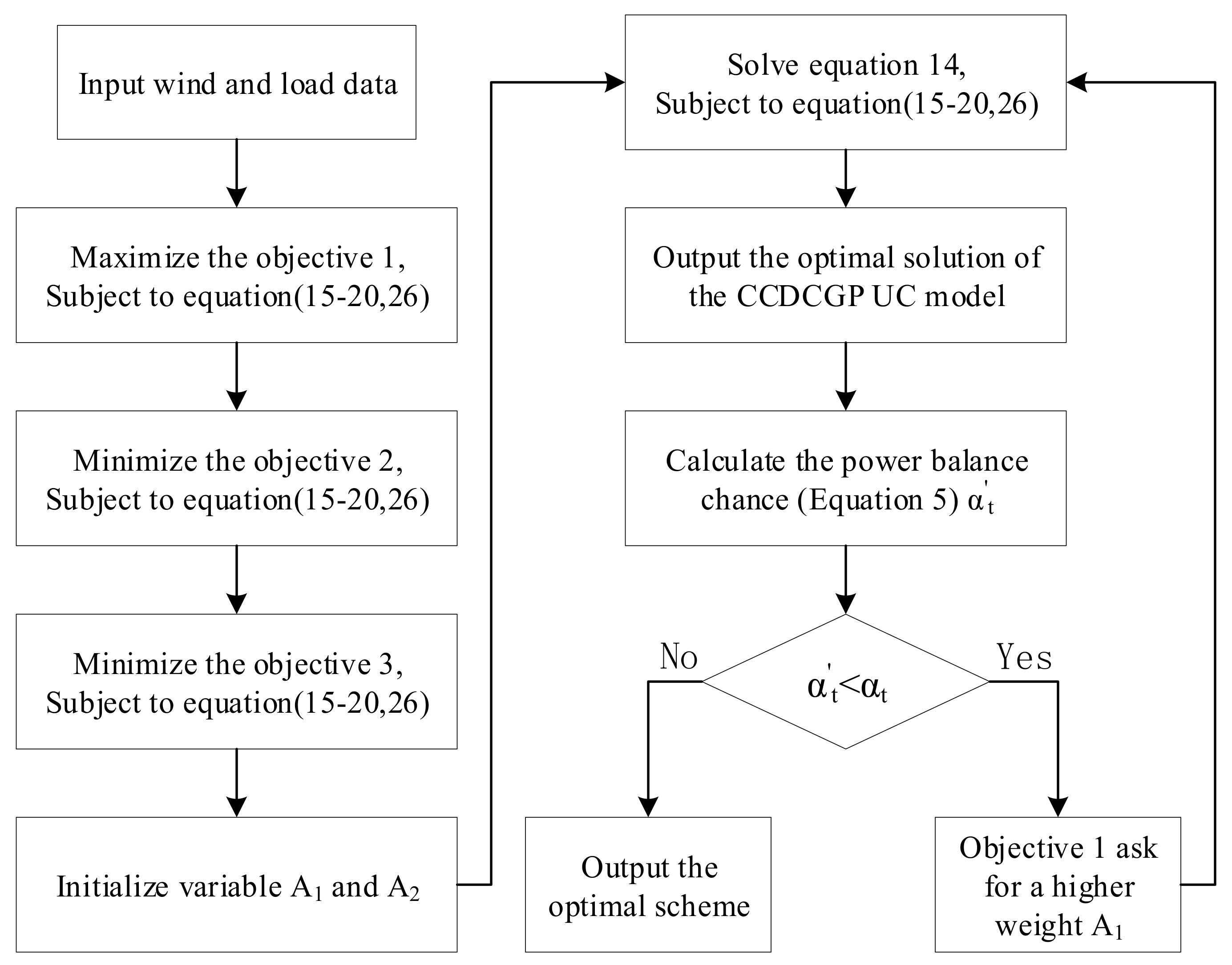
The flowchart for solving the proposed UC model is presented in Figure 4.

5. Case Study

5.1. Case Description

A modified 10-machine, 39-bus system is considered in this simulation to verify the feasibility and validity of the proposed model. The unit parameter data can be obtained from published material [27] which is given in [50], and the historical data of wind power and load forecast output are all scaled down by using Belgian grid data [51]. The wind power and load forecast values are shown in Figure 5, and wind farm Group 1, with an installed capacity of 500 MW, is located at bus 9, while wind farm Group 2, with an installed capacity of 800 MW, is located at bus 19. The optimisation is implemented using Cplex 12.6.3 on a DELL desktop machine with an Intel core i7-4790, 3.60 GHz processor, and 8 GB of random access memory.

5.2. Analysis of Results

5.2.1. Day-Ahead UC Scheme

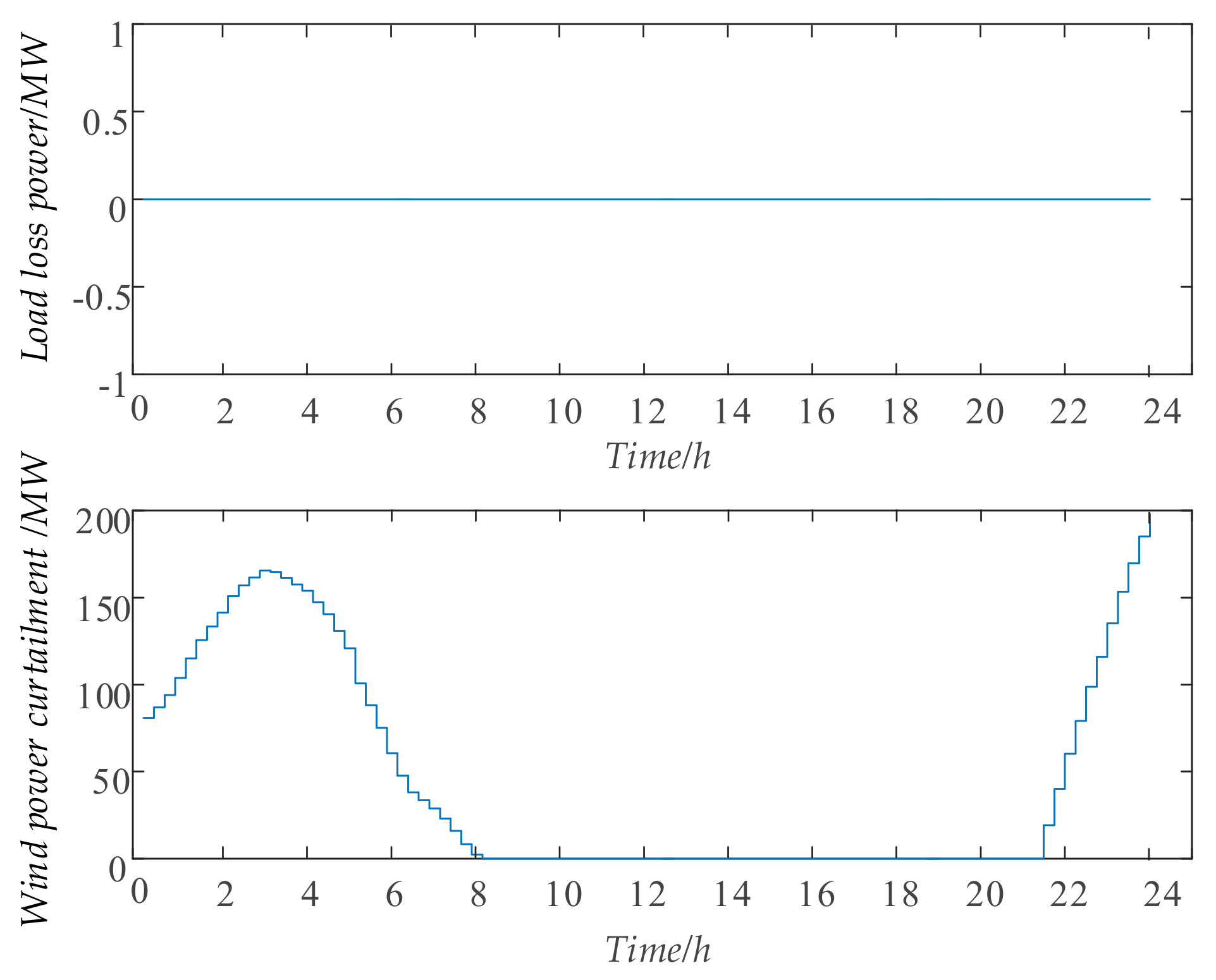
Under the premise of confidence level β 1 = β 2 = 0.96 , wind power curtailment of 1230.59 MW·h occurred due to the small capacity of most of the units and insufficient adjustment capacity. The total cost of the system is $254,487.53 and there is no load loss. The output of each generator is shown in Figure 6, and the wind power curtailment and load loss power are shown in Figure 7.
The figures show that, with the increase penetration rate of wind power, the uncertain power generated by wind power increases. To ensure safety of system operation, more units need to be kept on to provide spinning reserve capacity. It can be seen that, with the increase of renewable energy penetration rate, the system should increase the flexibility of operation to cope with the uncertainty of wind and photovoltaic power generation.

5.2.2. Model Validity Analysis

To verify the validity of the proposed chance-constrained dependent chance goal programming model, the following four models are adopted respectively for comparative simulation:
  • Model 1: conventional deterministic optimisation UC model. Power balance equation uses a conventional processing model that directly ignores forecast errors. To cope with the uncertainty of wind power, the spinning reserve requirement of the system is the sum of the load reserve capacity and 30% of the predicted wind power.
  • Model 2: stochastic optimisation UC model based on the scenario method. The processing approach of the power balance equation is to be balanced in each selected scenario. Adopting a Latin cube sampling strategy, dynamic scenario generation, and reduction techniques as described elsewhere [52], 10,000 initial scenarios are generated, and the 50 preserved scenarios optimised for calculation thereafter.
  • Model 3: stochastic optimisation UC model based on chance-constrained programming. The power balance equation uses a conventional processing model that directly ignores forecast errors. The confidence level for the establishment of the chance constraint of system positive and negative reserve power is β 1 = β 2 = 0.96 .
  • Model 4: the proposed chance-constrained dependent chance goal programming model. The power balance equation uses the processing model where the equality constraint is loosened to an inequality constraint and is then transformed into the chance-constrained dependent chance programming model. The confidence level for the establishment of the chance constraint of system positive and negative reserve power is β 1 = β 2 = 0.96 .
The computational performance is shown in Table 1, and results of the simulation using the aforementioned four optimisation UC models are summarised in Table 2.
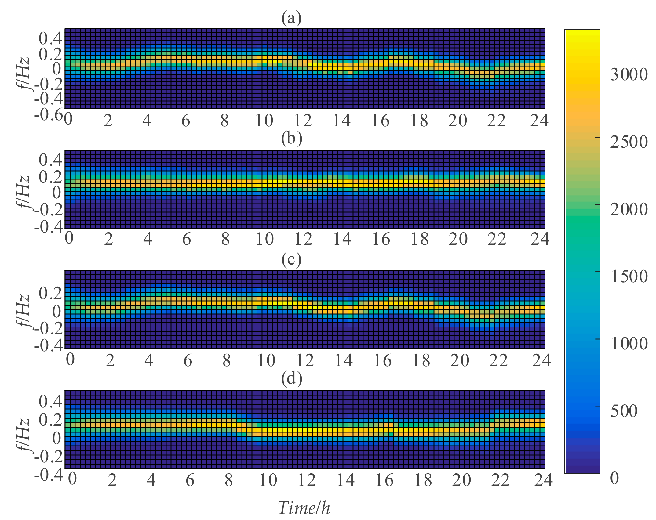
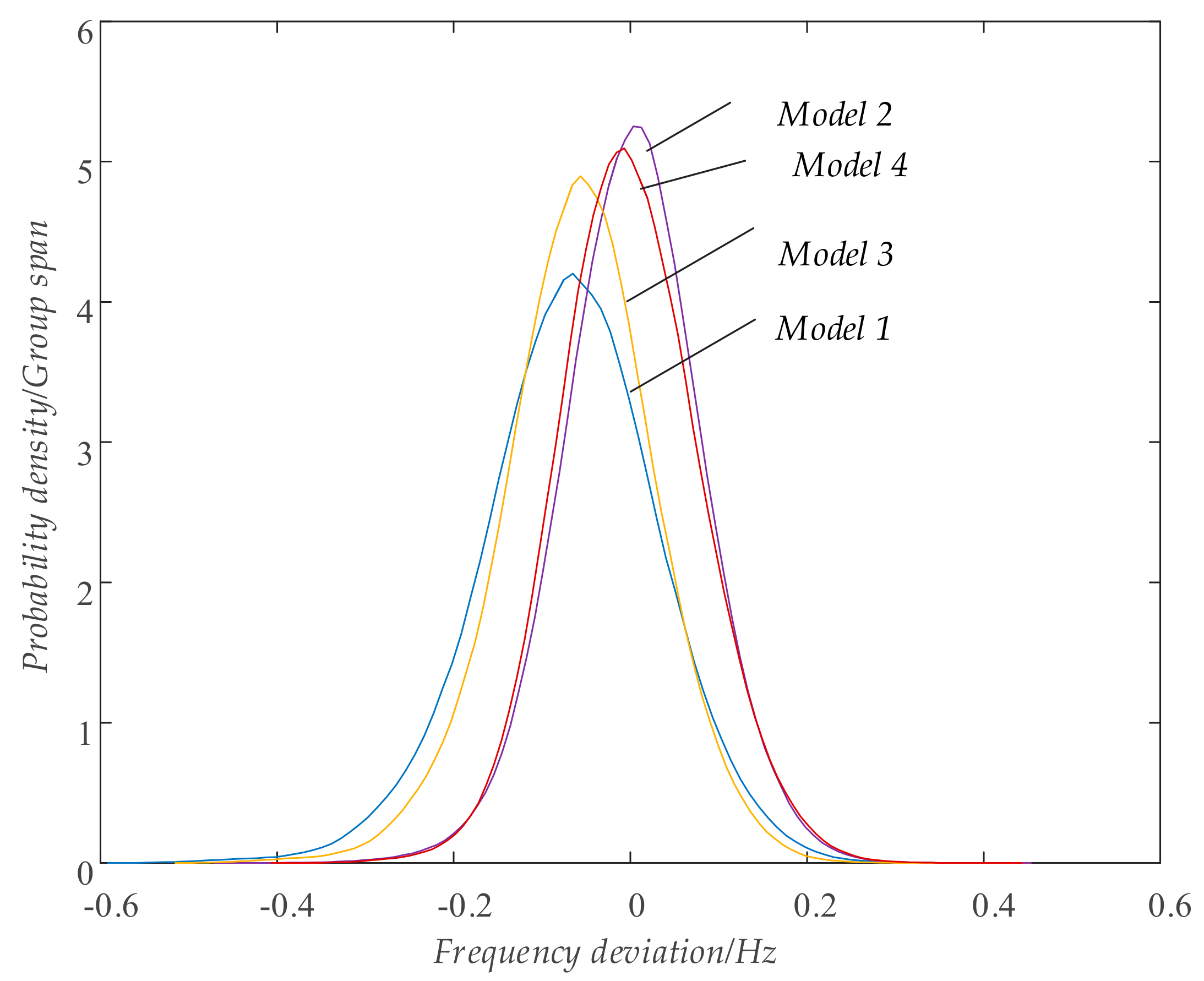
Table 1 shows the total cost of the simulation results of the proposed model is the smallest, and the amount of wind power curtailment is the least, while the solution time of Model 2, based on the scenario method, is significantly longer than that of other models. Without considering the adjustment of the intra-day UC scheme and automatic generation control (AGC) unit adjustment, possible wind power and load scenarios may be used to perform simulation operations according to the schedules formulated by each model. The power deviation between power supply and load can be used to test the effects of each power balance equation processing method. Under this power deviation, the frequency deviation under each scenario obtained by considering only inherent frequency modulation can reflect the ability of different models to respond to wind power and load uncertainty. Based on the probability distribution of wind power and load forecast errors, 10,000 possible scenarios of wind power and load are selected for simulation operation according to the schedules formulated by use of the four models. The statistical distribution of the power imbalance, under various models, and without considering the adjustment of the intra-day scheme and the adjustment of AGC units, is shown in Figure 8. The thermodynamic diagram of frequency deviation is shown in Figure 9, and the frequency deviation statistics are shown in Figure 10.
In Figure 8, the UC scheme of Model 1 and 3 simulates the coincidence of the probability density curves of power deviation during operation, and the distribution range is wide and the mean value is non-zero; the total power deviations of the UC schemes formulated by Models 2 and 4 are smaller than those using Models 1 and 3 during simulation, and the UC scheme formulated by Model 4 (i.e., that proposed in this paper) offers the best simulation performance. Due to the fact that the power balance equations of Models 1 and 3 directly ignore the influence of the forecast error, the power deviation of the UC scheme is a reflection of the power forecast error. Model 2, based on a scenario method, considers the error effects of 50 typical scenarios. Therefore, the errors in the selected 50 typical scenarios are modified when the UC scheme is formulated, and the overall effect is better than of Models 1 and 3 that do not consider the effects of forecast errors: however, due to the loss of forecast error information during the scenario reduction process, model 2 offers a poorer performance than dependent chance programming (Equation (6)) as proposed in this paper.
The power deviation mean values of UC schemes formulated by Models 1 and 3 (Figure 8) are positive during simulation runs. It can be shown that the output power of the thermal units of Models 1 and 3 is generally small without considering the forecast error when formulating the UC scheme, while the thermal units of Models 2 and 4, considering the actual output of wind power, need to generate more power to balance the deviation between the forecast output and the actual output of wind power. This leads to a higher total cost of the actual operation of the UC scheme formulated by Models 1 and 3, and the curtailment of wind power decreases in relative terms. To confirm the above assumptions, the mean value of the forecast error is added to the power balance equations of Models 1 and 3 (Equation (4)). The total cost of Model 1 is $273,745.80, and the wind power curtailment is 1869.76 MW·h; while the total cost of Model 3 is $275,787.48, and the wind power curtailment is 1816.04 MW·h. So far, the correctness of the above assumptions has been proved. From Figure 9 and Figure 10, the frequency deviations of the UC schemes formulated by Models 1 and 3 are quite different when facing the same power deviation, and the ability of Model 3 to cope with power uncertainty is better than that of Model 1.
Excluding the factor whereby the total output of the thermal units is unequal as caused by the forecast error mean value being non-zero (the total cost and the wind power curtailment of Model 1 are $273,745.80 and 1869.76 MW·h, respectively, while the total cost and the wind power curtailment of Model 3 are $275,787.48 and 1816.04 MW·h, respectively), the proposed UC scheme is economically dominant and suffers the smallest amount of wind power curtailment. It is no longer limited to the same power supply and load power forecast value in the power balance equation of the optimisation model, so the optimisation can be performed in a wider space. Therefore, the objective function of the obtained solution must not be worse than the original. The power balance equation (Equation (2)), which has the same power supply and load forecast value, only corresponds to a possible scenario where the forecast error is zero during the actual execution, but it reduces the search space by one dimension. From Figure 8, Figure 9 and Figure 10, the power balance equation proposed here is loosened to an inequality formula with small out-of-balance errors, and the adoption of the dependent chance programming model does not introduce the risk of power imbalance to the system. On the contrary, due to having considered that as many realistic possible output scenarios as possible can satisfy the loosened power balance equation, the obtained solution has unique advantages in dealing with wind power and load imbalance power.
Figure 10 shows that the stochastic optimisation UC method offers advantages in dealing with the uncertainty of wind power output. Due to the power balance equation considering the uncertainty of forecast errors during the UC modelling process, the scenario method and the proposed method perform well. In most scenarios, the frequency deviation is within ±0.2 Hz.

5.2.3. Sensitivity Analysis

From the modelling process, it can be seen that the proposed power balance processing method introduces a key variable σ, which represents the power imbalance in Equation (5). This variable directly affects the size of the feasible set in the constructed uncertain environment, thus affecting the formulation of the UC scheme. To determine the impact of the power imbalance σ on the UC scheme, the UC model is solved for different values of σ. The load loss under different power imbalances σ is zero, and the total cost and the amount of wind power curtailment are as shown in Figure 11.
The figure shows that with the increase in power imbalance σ, the cost of the scheme and the amount of wind power curtailment increase, and the effect of σ on wind power curtailment is more significant than that of the cost. This is because, with the increase in σ, the span of the feasible set in the uncertain environment is increasing, and the probability of the establishment of Equation (5) is increasing. Since the objective function optimises objective function f 1 with the highest priority, the output arrangement of the thermal units at this time guarantees the power balance represented by Equation (6) with the highest probability. On this basis, the economy and renewable energy consumption ability are considered. Therefore, the cost and the amount of wind power curtailment will increase with σ; however, with the increase of the power imbalance σ, the size of the feasible set under the uncertain environment increases, so that more wind power and load error scenarios meet the requirements of Equation (5), which improves the ability of system to cope with uncertain power and the security of system operation. The power deviation and frequency deviation statistics under different σ-simulation operation scenarios are shown in Figure 12 and Figure 13.
From the figure, as the value of σ increases, the power deviation and frequency deviation under the simulated operation scenario both decrease. This shows that, with the increase in σ, although the economy of system operation and the renewable energy consumption capacity are decreasing, the ability of the system to cope with uncertain power is increasing, and system operation is more secure.

6. Discussion

The above mentioned tables and figures can be summed up as follows:
  • Excluding the factor whereby the total output of the thermal units is unequal as caused by the forecast error mean value being non-zero, the proposed UC scheme is economically dominant and suffers the smallest amount of wind power curtailment.
  • From the simulation results, the UC models formulated by the power balance equation that do not consider the impact of forecast errors completely have a larger deviation of power supply and load than the UC models that consider the impact of forecast errors in the power balance equation. In the UC models that consider the impact of forecast errors in the power balance equation, the proposed UC model performs better than the stochastic UC model based on scenarios. This is because the stochastic UC model based scenarios make the UC scheme based on the error distribution information obtained from the reserved scenarios, while the UC model proposed in this paper directly makes the UC scheme by using the original error distribution information, and there is no error in the expression of the forecast error distribution information caused by the scenario reduction process.
  • Compared with the conventional method processing power balance equation in which the power supply predicted value is equal to load predicted value, the method proposed in this paper expands the search space of the optimization model. The obtained UC scheme can significantly improve not only operation efficiency and wind power consumption, but also the balance level of power supply and demand after considering the forecast error.
  • The model proposed in this paper for processing the power balance equation with uncertain variables does not bring a power imbalance risk to the system, though the equality constraint is loosened to an inequality constraint with small imbalance errors and then solved by dependent chance programming. In contrast, considering as many realistic possible output scenarios as possible can satisfy the loosened power balance equation, therefore, the obtained solution has unique advantages in dealing with the uncertainty of wind power and load.
  • When using the dependent chance programming model proposed in this paper to deal with the power balance equation containing wind power and load forecast errors, a smaller power imbalance σ is not necessarily better. Since the proposed model optimizes the objective function 1 which represents the “power balance” with the highest priority, a larger σ within a certain range does not deteriorate the imbalance of power supply and demand when the UC scheme is actually operated. On the contrary, due to the increase of σ, the feasible set under the uncertain environment is expanded, so that more wind power and load error scenarios meet the “power balance” defined by Equation (5), and the ability of the system to cope with uncertain power is improved. The negative effect is to increase the operation cost of the scheme and reduce the capacity of wind power consumption.

7. Conclusions

We considered the influence of forecast errors in the power balance equation of a power system UC model, and the problem of processing the power balance equation with uncertain variables was studied. A power system day-ahead optimisation UC model based on chance-constrained dependent chance programming was established to solve a power balance equation containing random variables. The following conclusions were obtained:
  • The forecast errors of wind power and load in the power balance equation of the power system UC model will directly affect the formulation of the UC scheme. In particular, when the forecast error mean value is non-zero, the influence will be greater, and the effects will be greater with the increase in the scale of wind power generation.
  • In power systems with large-scale, uncertain power supplies, the power balance equation in the UC model is loosened to an inequality constraint, and the chance-constrained dependent chance goal programming model proposed in this paper is used in the formulation of the solution. During practical operation of the obtained UC scheme, instead of getting larger, the power deviation will be smaller than that scheduled by the equation that only considers the predicted value.
Sensitivity analysis illustrates how the operation efficiency and wind power consumption can be represented through the power imbalance σ, and this has significant impact on the result. Directions for future work include investigating the influence of forecast error distributions on the power balance objective function 1 and the accurate description of wind power forecast error.

Author Contributions

S.Z. and Z.L. conceived and designed the experiments; Z.L. performed the experiments; S.Z. and Z.L. analysed the data; Z.L. and T.J. wrote the paper; J.L. provided the wind farm data.

Funding

This paper is supported by National Key Research and Development Program of China (2017YFB0902200), State Grid Corporation of China (5228001700CW), and Fundamental Research Funds for the Central Universities (2018QN074).

Conflicts of Interest

The authors declare no conflict of interest.

References

  1. Koltsaklis, N.E.; Dagoumas, A.S.; Georgiadis, M.C.; Papaioannou, G.; Dikaiakos, C. A mid-term market-based power systems planning model. Appl. Energy 2016, 179, 17–35. [Google Scholar] [CrossRef]
  2. Smith, J.C.; Milligan, M.R.; DeMeo, E.A.; Parsons, B. Utility wind integration and operating impact state of the art. IEEE Trans. Power Syst. 2007, 22, 900–908. [Google Scholar] [CrossRef]
  3. Sperati, S.; Alessandrini, S.; Pinson, P.; Kariniotakis, G. The “Weather Intelligence for Renewable Energies” benchmarking exercise on short-term forecasting of wind and solar power generation. Energies 2015, 8, 9594–9619. [Google Scholar] [CrossRef] [Green Version]
  4. Cadenas, E.; Rivera, W.; Campos-Amezcua, R.; Heard, C. Wind speed prediction using a univariate ARIMA model and a multivariate NARX model. Energies 2016, 9, 109. [Google Scholar] [CrossRef]
  5. Marneris, G.I.; Biskas, N.P.; Bakirtzis, G.A. Stochastic and deterministic unit commitment considering uncertainty and variability reserves for high renewable integration. Energies 2017, 10, 140. [Google Scholar] [CrossRef]
  6. Trombe, P.-J.; Pinson, P.; Madsen, H. A general probabilistic forecasting framework for offshore wind power fluctuations. Energies 2012, 5, 621–657. [Google Scholar] [CrossRef] [Green Version]
  7. Wang, C.; Li, X.; Wang, Z.; Dong, X.; Liang, Z.; Liu, X.; Liang, J.; Han, X. Day-ahead unit commitment method considering time sequence feature of wind power forecast error. Int. J. Electr. Power Energy Syst. 2018, 98, 156–166. [Google Scholar] [CrossRef]
  8. Wang, G.; You, D.; Zhang, Z.; Dai, L.; Zou, Q.; Liu, H. Network-constrained unit commitment based on reserve models fully considering the stochastic characteristics of wind power. Energies 2018, 11, 435. [Google Scholar] [CrossRef]
  9. Wang, C.; Liu, F.; Wang, J.; Qiu, F.; Wei, W.; Mei, S.; Lei, S. Robust risk-constrained unit commitment with large-scale wind generation: an adjustable uncertainty set approach. IEEE Trans. Power Syst. 2017, 32, 723–733. [Google Scholar] [CrossRef]
  10. Zhao, C.; Wang, J.; Watson, J.-P.; Guan, Y. Multi-stage robust unit commitment considering wind and demand response uncertainties. IEEE Trans Power Syst. 2013, 28, 2708–2717. [Google Scholar] [CrossRef]
  11. Kiran, B.D.H.; Kumari, M.S. Demand response and pumped hydro storage scheduling for balancing wind power uncertainties: A probabilistic unit commitment approach. Int. J. Electr. Power Energy Syst. 2016, 81, 114–122. [Google Scholar] [CrossRef]
  12. Zhao, J.; Wan, C.; Xu, Z.; Wong, K.P. Spinning reserve requirement optimization considering integration of plug-in electric vehicles. IEEE Trans. Smart Grid 2017, 8, 2009–2021. [Google Scholar] [CrossRef]
  13. Park, H.-G.; Lyu, J.-K.; Kang, Y.; Park, J.-K. Unit Commitment considering interruptible load for power system operation with wind power. Energies 2014, 7, 4281–4299. [Google Scholar] [CrossRef]
  14. Wang, J.; Botterud, A.; Bessa, R.; Keko, H.; Carvalho, L.; Issicaba, D.; Sumaili, J.; Miranda, V. Wind power forecasting uncertainty and unit commitment. Appl. Energy 2011, 88, 4014–4023. [Google Scholar] [CrossRef]
  15. Abujarad, S.Y.; Mustafa, M.W.; Jamian, J.J. Recent approaches of unit commitment in the presence of intermittent renewable energy resources: A review. Renew. Sustain. Energy Rev. 2017, 70, 215–223. [Google Scholar] [CrossRef]
  16. Liu, D.; Guo, J.; Huang, Y. Dynamic economic dispatch of wind integrated power systems based on wind power probabilistic forecasting and operation risk constraints. Proc. CSEE 2013, 33, 9–15. [Google Scholar]
  17. Zhan, Z.; Sun, Y.; Gao, D.; Lin, J.; Cheng, L. A versatile probability distribution model for wind power forecast errors and its application in economic dispatch. IEEE Trans. Power Syst. 2013, 28, 3114–3125. [Google Scholar] [CrossRef]
  18. Qin, N.; Bak, C.L.; Abildgaard, H.; Chen, Z. Multi-Stage optimization-based automatic voltage control systems considering wind power forecasting errors. IEEE Trans. Power Syst. 2017, 32, 1073–1088. [Google Scholar] [CrossRef]
  19. Bertsimas, D.; Litvinov, E.; Sun, X.A.; Zhao, J.; Zheng, T. Adaptive robust optimization for the security constrained unit commitment problem. IEEE Trans. Power Syst. 2013, 28, 52–63. [Google Scholar] [CrossRef]
  20. Ruiz, P.A.; Philbrick, C.R.; Zak, E.; Cheung, K.W.; Sauer, P.W. Uncertainty management in the unit commitment problem. IEEE Trans. Power Syst. 2009, 24, 642–651. [Google Scholar] [CrossRef]
  21. Jiang, R.; Wang, J.; Guan, Y. Robust unit commitment with wind power and pumped storage hydro. IEEE Trans. Power Syst. 2012, 27, 800–810. [Google Scholar] [CrossRef]
  22. Wang, Y.; Xia, Q.; Kang, C. Unit commitment with volatile node injections by using interval optimization. IEEE Trans. Power Syst. 2011, 26, 1705–1713. [Google Scholar] [CrossRef]
  23. Pandzic, H.; Dvorkin, Y.; Qiu, T.; Wang, Y.; Kirschen, D.S. Toward cost-efficient and reliable unit commitment under uncertainty. IEEE Trans. Power Syst. 2015, 99, 1–13. [Google Scholar]
  24. Charnes, A.; Cooper, W.W. Chance-constrained programming. Manag. Sci. 1959, 6, 73–79. [Google Scholar] [CrossRef]
  25. Wu, H.; Shahidehpour, M.; Li, Z.; Tian, W. Chance-constrained day-ahead scheduling in stochastic power system operation. IEEE Trans. Power Syst. 2014, 29, 1583–1591. [Google Scholar] [CrossRef]
  26. Wang, Q.; Guan, Y.; Wang, J. A chance-constrained two-stage stochastic program for Unit commitment with uncertain wind power output. IEEE Trans. Power Syst. 2012, 27, 206–215. [Google Scholar] [CrossRef]
  27. Wang, Y.; Zhao, S.; Zhou, Z.; Botterud, A.; Xu, Y.; Chen, R. Risk adjustable day-ahead unit commitment with wind power based on chance constrained goal programming. IEEE Trans. Sustain. Energy 2017, 8, 530–541. [Google Scholar] [CrossRef]
  28. Wu, L.; Shahidehpour, M.; Li, T. Stochastic security-constrained unit commitment. IEEE Trans. Power Syst. 2007, 22, 800–811. [Google Scholar] [CrossRef]
  29. Pinson, P.; Madsen, H.; Nielsen, H.; Papaefthymiou, G.; Klöckl, B. From probabilistic forecasts to statistical scenarios of short-term wind power production. Wind Energy 2009, 12, 51–62. [Google Scholar] [CrossRef] [Green Version]
  30. Wu, L.; Shahidehpour, M.; Li, Z. Comparison of scenario-based and interval optimization approaches to stochastic SCUC. IEEE Trans. Power Syst. 2012, 27, 913–921. [Google Scholar] [CrossRef]
  31. Bai, W.; Lee, D.; Lee, K.Y. Stochastic dynamic AC optimal power flow based on a multivariate short-term wind power scenario forecasting model. Energies 2017, 10, 2138. [Google Scholar] [CrossRef]
  32. Growe-Kuska, N.; Heitsch, H.; Romisch, W. Scenario reduction and scenario tree construction for power management problems. In Proceedings of the IEEE Bologna Power Tech Conference, Bologna, Italy, 23–26 June 2003. [Google Scholar] [Green Version]
  33. Dupačová, J.; Gröwe-Kuska, N.; Römisch, W. Scenario reduction in stochastic programming: An approach using probability metrics. Math. Progr. 2003, 95, 493–511. [Google Scholar] [CrossRef]
  34. Huang, Y.; Zheng, Q.P.; Wang, J. Two-stage stochastic unit commitment model including non-generation resources with conditional value-at-risk constraints. Electr. Power Syst. Res. 2014, 116, 427–438. [Google Scholar] [CrossRef]
  35. Zhao, C.; Guan, Y. Unified stochastic and robust unit commitment. IEEE Trans. Power Syst. 2013, 28, 3353–3361. [Google Scholar] [CrossRef]
  36. Dvorkin, Y.; Pandzic, H.; Ortega-Vazquez, M.A.; Kirschen, D.S. A hybrid stochastic/interval approach to transmission-constrained unit commitment. IEEE Trans. Power Syst. 2015, 30, 621–631. [Google Scholar] [CrossRef]
  37. Koltsaklis, N.E.; Georgiadis, M.C. A multi-period, multi-regional generation expansion planning model incorporating unit commitment constraints. Appl. Energy 2015, 158, 310–331. [Google Scholar] [CrossRef]
  38. Che, L.; Liu, X.; Li, Z. An intrainterval security risk regarding regulation burden due to wind variation in high-wind-penetrated power systems. IEEE Trans. Power Syst. 2018, 33, 3213–3216. [Google Scholar] [CrossRef]
  39. Wang, J.; Shahidehpour, M.; Li, Z. Security-constrained unit commitment with volatile wind power generation. IEEE Trans. Power Syst. 2008, 23, 1319–1327. [Google Scholar] [CrossRef]
  40. Xu, Q.; He, D.; Zhang, N.; Kang, C.; Xia, Q.; Bai, J.; Huang, J. A short-term wind power forecasting approach with adjustment of numerical weather prediction input by data mining. IEEE Trans. Sustain. Energy 2015, 6, 1283–1291. [Google Scholar] [CrossRef]
  41. Methaprayoon, K.; Yingvivatanapong, C.; Lee, W.-J.; Liao, J.R. An Integration of ANN Wind Power Estimation into Unit Commitment Considering the Forecasting Uncertainty. IEEE Trans. Ind. Appl. 2007, 43, 1441–1448. [Google Scholar] [CrossRef]
  42. Shen, Z.; Wu, X.; Guerrero, J.M.; Song, Y. Model-independent approach for short-term electric load forecasting with guaranteed error convergence. IET Control Theory Appl. 2015, 10, 1365–1373. [Google Scholar] [CrossRef]
  43. Cai, G.; Wang, W.; Lu, J. A Novel Hybrid Short Term Load Forecasting Model Considering the Error of Numerical Weather Prediction. Energy 2016, 9, 994. [Google Scholar] [CrossRef]
  44. Xia, C.; Wang, J.; McMenemy, K. Short, medium and long term load forecasting model and virtual load forecaster based on radial basis function neural networks. Int. J. Electr. Power Energy Syst. 2010, 32, 743–750. [Google Scholar] [CrossRef] [Green Version]
  45. Ortega-Vazquez, M.A.; Kirschen, D.S. Estimating the Spinning Reserve Requirements in Systems with Significant Wind Power Generation Penetration. IEEE Trans. Power Syst. 2009, 24, 114–124. [Google Scholar] [CrossRef]
  46. Bouffard, F.; Galiana, F.D. Stochastic Security for Operations Planning with Significant Wind Power Generation. IEEE Trans. Power Syst. 2008, 23, 306–316. [Google Scholar] [CrossRef]
  47. Liu, B. Dependent-chance programming: A class of stochastic programming. Comput. Math. Anal. Appl. 1996, 199, 293–311. [Google Scholar]
  48. Zhou, W.; Sun, H.; Gu, H. Dynamic economic dispatch of wind integrated power systems based on risk reserve constraints. Proc. CSEE 2012, 32, 47–55. [Google Scholar]
  49. Li, Z.; Zhao, S.; Li, D.; Zhang, T. Fast solving of day-ahead power system scheduling chance-constrained model based on improved ε-constrained and deterministic transform by sampling. Proc. CSEE 2018, 38, 1–13. [Google Scholar]
  50. Unit Parameter Data. Available online: https://docs.google.Com/document/d/1jKJNnvIp5hURLiez Umr9ewiMI4vQjCqscUuvY0bgB30/pub (accessed on 18 April 2018).
  51. Elia. Wind-Power Generation Data & Solar-PV Power Generation Data. Available online: http://www.elia.be/en/grid-data/power-generation/wind-power (accessed on 15 July 2017).
  52. Ma, X. Scenario Analysis and Stochastic Programming of Wind-Integrated Power Systems. Ph.D. Thesis, Wuhan University, Wuhan, China, 2014. [Google Scholar]
Figure 1. Forecast error of wind power and load.
Energies 11 01718 g001
Figure 2. Thermodynamic diagram of wind and load actual power scenario.
Energies 11 01718 g002
Figure 3. Flow chart of the proposed unit commitment (UC). MIQP: mixed integer quadratic programming; MILP: mixed integer linear programming.
Energies 11 01718 g003
Figure 4. Flowchart for solving the proposed UC model. CCDCGP: chance-constrained dependent chance goal programming.
Energies 11 01718 g004
Figure 5. Wind farm and load forecast power.
Energies 11 01718 g005
Figure 6. Each generation unit output.
Energies 11 01718 g006
Figure 7. Wind power curtailment and load loss in optimal UC.
Energies 11 01718 g007
Figure 8. Power deviation statistics of four types of UC schemes.
Energies 11 01718 g008
Figure 9. Thermodynamic diagram of frequency deviation of four types of UC schemes.
Energies 11 01718 g009
Figure 10. Frequency deviation statistics of four types of UC schemes.
Energies 11 01718 g010
Figure 11. Total cost of the scheme and the change of wind power curtailment vary with σ.
Energies 11 01718 g011
Figure 12. Power deviation statistics under simulated operation scenarios under different power imbalances σ.
Energies 11 01718 g012
Figure 13. Frequency deviation statistics under simulated operation scenarios under different power imbalances σ.
Energies 11 01718 g013
Table 1. Computational performance of different UC model.
UC ModelVariableConstraint ConditionComputing Time/s
Model 1220813,70836.53
Model 220,448212,524367.27
Model 3220813,70830.75
Model 4220813,61224.65
Table 2. Different UC model optimisation results.
UC SchemeTotal Cost/DollarWind Power Curtailment/MW·hLoad Loss Power/MW·h
Model 1259,745.752411.660
Model 2259,752.351743.170
Model 3254,609.162311.270
Model 4254,487.531230.590