1. Introduction
The Doubly Fed Induction Generator (DFIG) has been widely used in wind energy generation systems (WEGs), because the capability of its power converter is only about one third the wind turbine power rating [
1], but the slip rings and electro-brushes of the DFIG lead to frequent maintenance and increases the system cost, especially for offshore wind farms [
2]. The Brushless Doubly Fed Induction Machine (BDFIM) has the outstanding features of no slip rings and electro-brushes, resulting in more robustness and durability than the DFIG [
3,
4,
5]. Furthermore, the BDFIM has two stators, denoted as the power winding (PW) stator and the control winding (CW) stator, and a special designed rotor, where the rotor has two kinds of structures as the squirrel-cage type and the wound-rotor type [
6]. On the other hand, the BDFIM is equivalent to the DFIG in function, which makes the BDFIM is more attractive in terms of the WEG applications [
7,
8,
9].
In terms of the BDFIM control methods, the scalar control has no feedback link and it is difficult to obtain a fast dynamic response [
10]. The direct power control [
11] and the indirect control scheme [
12] directly regulate the speed or power by the amplitude and angle of the CW flux, while good dynamic responses are questionable due to the lack of timely current adjustment; on the other hand, direct control methods [
13,
14,
15] require high switching frequency to reduce torque ripples and relies on accurate estimations of torque or flux, thus the vector control method is preferred due to simple control structure and easy implementation. In addition, the single-loop control method simplifies the control algorithm at the sacrifices of tracking performance [
16], the vector control with the inner current controller is more commonly used in drive system, where the inner current sub-system is designed as a small time constant system in order to achieve good dynamics.
In the inner current sub-system of the BDFIM, complex cross-coupling terms, the back electromotive force (EMF) disturbance and parametric errors increase the difficulty of the controller design and decrease the control performance [
17,
18,
19], while the previous current control methods of the BDFIM have not addressed the problems caused by parametric errors. In addition, effects of complex coupling terms are usually eliminated or suppressed by combining the conventional PI controller and the feedforward control. Different feedforward compensation terms generate diverse total resistances and total leakage inductances of the current sub-system, which directly affect the current controller design and the control performance. In [
17] the feedforward component consists of the CW flux, the PW flux, and the CW current; In [
18], the PW flux, the derivative of the PW flux, the PW current and the CW current make up the feedforward component; while the feedforward terms are calculated by the PW current, CW current and their derivatives in [
19]. However, these feedforward terms are very complex, and the compensation performance is guaranteed by precise motor parameters and calculations especially when the derivatives of the current are included. In addition, the above controllers are designed based on the CW resistance of the BDFIM, which is impossible to measure accurately. Simple controller is designed by neglecting the rotor resistance [
20], but effects of the rotor resistance on the current controller of the BDFIM are not taken into accounts, which inevitably reduces the control performance [
21,
22,
23].
In order to address the problems caused by complex coupling terms and parametric errors and enhance the robustness and dynamic responses of the current controller, an internal model current control strategy with the “active resistance” is proposed in this paper, where effects of the rotor resistance are reduced. In this method, the slow timescale dynamics of the flux sub-system are studied based on the state space mathematical model of the BDFIM, and a detailed design procedure of the current controller is discussed. Also, when the symmetrical PW voltage sag happens, an EMF feedforward term composed by the grid voltage is added in the current controller. Furthermore, the machine parameters are estimated, and the influences of erroneous parameters on the current controller are studied.
This paper is organized as follows: an introduction to the current controller of the BDFIM is discussed in
Section 1. The state-space model of the BDFIM in the PW
dq synchronous reference frame is introduced in
Section 2, and then the dynamics of the flux sub-system is studied. A CW current controller based on the internal model control method is designed in
Section 3. The BDFIM parameters are estimated and their effects on the CW current controller are studied in
Section 4. Simulation and experimental results are presented in
Section 5. Discussions on the feasibility of the proposed method are given in
Section 6. Finally, the conclusions are derived in
Section 7.
2. System Configuration and Mathematical Model of the BDFIM
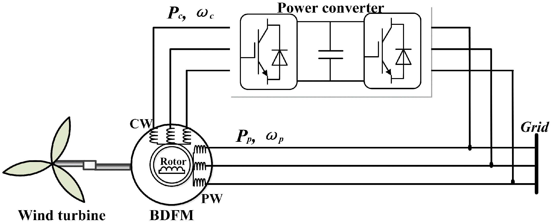
The schematic diagram of the BDFIM system is described in
Figure 1, where the BDFIM is composed of the PW stator, the CW stator, and the rotor. Usually, the harmonic orders and its components of the rotor windings of the wound-rotor type rotor BDFIM are relatively reduced, and the motor efficiency is high, thus the wound-rotor-type BDFIM is studied in this paper. However, the proposed method is also useful for the first type, because only the fundamental magnetic potential determines the controller design here. The power grid directly connects the BDFIM by the PW stator, and the transformer outputs a suitable voltage to meet the grid-connected requirement. In this system, the BDFIM is regulated by pouring the expected current into the CW stator, and these currents are generated by the power converter.
2.1. Grid-Flux Orientation
In order to realize the vector control scheme, all the quantities are oriented in the reference frame, which is aligned with a flux linkage. In terms of the DFIG system, in contrast to stator-flux orientation, the flux dynamics and system stability are independent of the rotor current by using grid-flux orientation, while they are equal in the steady state because the stator resistance is neglectable [
24]. Similarly, considering the above features, the BDFIM control is discussed in the grid-flux orientation frame, the
dq components of the grid-flux are
φgd = |
φg| and
φgq = 0, where
φgd and
φgq are the
dq components of the grid-flux
φg. The orientation angle, denoted as
θF, is calculated as:
where
θg is the angle of grid voltage
vg and obtained by a phase-locked loop (PLL) estimator.
In this case, a dq synchronous reference frame is built by and , where x is the arbitrary variable, the superscripts “dq”, “d”, “q” represent the dq frame, d-axis component and q-axis component, respectively. Then, the rotor current and rotor flux are written as , , where Pp is the number of pole pairs of the PW stator, δ1 is the initial angular position between PW stator and the rotor, and θr is the mechanical rotor angle. The PW and CW variables are , , where “*” represents the conjugate of the vector, the subscripts “p” and “c” represent the PW and the CW, Pc is the number of pole pairs of the CW stator, δ2 is the initial angular position between CW stator and the rotor, the superscripts “αβp” and “αβc” are the stationary coordinate systems of the PW stator and the CW stator, respectively.
2.2. Mathematical Model of the BDFIM
On the basis of the grid-flux orientation frame, the basic mathematical model of the BDFIM [
25] is expressed as:
where,
v,
i and
ψ are the voltage, current and flux;
R,
L and
M are the resistance, self-inductance and mutual inductance; the subscript “
r“ represent the rotor;
ωp and
ωc are the electric angle frequencies of the PW stator and the CW stator, and
ωr is the mechanical angular frequency of rotor, respectively.
Taking the CW stator current
ic, the PW stator flux
ψp and the rotor flux
ψr as state variables, the state-space BDFIM model is derived from Equations (2)–(7), and it is given as:
where
Lσ and
Rt are the equivalent leakage inductance and equivalent total resistance;
ωslc is the slip frequency of the CW stator and
ωslc =
ωp − (
Pp +
Pc)
ωr;
Xψ,
Aψ, and
Bψ are the state matrix, the dynamic matrix and the input matrix, and
,
,
;
E is the back electromotive force and
; the detailed parameters are given in
Appendix.
As shown in Equations (8) and (9), the BDFIM is a multi-variable system (containing PW stator flux, rotor flux, and the CW current), which consists of the current sub-system and the flux sub-system. In order to independently analyze and control the current sub-system, the stability of the flux sub-system is subsequently discussed.
2.3. Stability Analysis of the Flux Sub-System
In the flux sub-system, the poles of the system transfer function are placed at the eigenvalues of Aψ, while the system is stable when the poles are located on the left half-plane. However, it is difficult to directly obtain the poles. In this case, the Routh-Hurwitz stability criterion is adopted to estimate the range of the poles.
Usually, the Routh-Hurwitz stability criterion is used in the vector spaces with real numbers, then the matrix
is transformed to
, which is expressed as:
where
,
.
The characteristic polynomial of
is expressed as:
where
.
Then, a set of four determinants is achieved from coefficients of 4th-degree characteristic polynomial Equation (11), and the coefficients used to estimate the system stability are expressed as:
where
,
.
Obviously, the coefficients in (12) are positive and D1 > 0, D2 > 0, D3 > 0, D4 > 0, thus the stability conditions are satisfied according to the Routh-Hurwitz stability criterion, and the real parts of eigenvalues of are negative.
In order to estimate the range of poles of the flux sub-system, a new characteristic polynomial equation is constructed by adding
δI2 to
, which is expressed as:
The coefficients of Equation (13) are calculated as:
Similarly, the new system is stable since all the coefficients in Equation (14) are positive, and the eigenvalues of Equation (13) are located on the left half-plane. Normally, the eigenvalues of N and -N are symmetric about the imaginary axis, real parts of the eigenvalues of are consequently larger than −δ, and real components of the poles of flux dynamic system Equation (10) are placed between −δ and zero on the left half-plane.
Without loss of generality, the CW current loop is designed as a high-gain feedback system, and then the DFIG system described by Equations (8) and (9) is a singularly perturbed system, where the fluxes are considered as the slowly varying variables and the current has a fast timescale dynamic. Since the flux sub-system is stable as discussed above, the current sub-system can be dependently controlled, where the fluxes are assumed in the steady-state. More details about the current controller design are given in the following part.
3. Design of the CW Current Controller
In the BDFIM drive system, both the power generation and rotor speed control can be achieved by properly adjusting the CW current as discussed in [
22,
25,
26], where a well-designed current controller is a prerequisite for the normal operation of the BDFIM system. In this part, the design details of the CW current controller are discussed, which aims to track the CW current command under the disturbance of the coupling terms and BDFIM parametric errors as shown in Equation (8). In order to achieve this aim, the proposed current controller is designed based on the internal model method [
27], and an active damping controller is added to increase the robustness of the system.
3.1. Internal Model Current Control
By applying the Laplace transform, the current sub-system Equation (8) is expressed as:
where
Y(
s) and
U(
s) are the system input and the system output respectively, and they are
and
,
icd,
icq,
vcd and
vcq are the
d-axis component and
q-axis component of
ic and
vc, respectively;
G(
s) is the controller system and
;
is the back EMF and
, where
ψpd,
ψpq,
ψrd,
ψrq,
vpd and
vpq are the
d-axis component and
q-axis compent of
ψp,
ψr and
vp, respectively.
The typical internal model control diagram is shown in
Figure 2,
R(s) is the system input reference and
,
is the internal model of the current sub-system, and
FIMC(
s) is the equivalent current controller, where
CIMC(
s) is the internal model controller and it is usually designed as:
where
LR(
s) is the feedforward filter designed to enhance the controller robustness.
It can be seen from Equation (8) that the current sub-system is a first-order system, then
LR(
s) is designed to be a first-order filter and it is expressed as:
where
αb is the desired closed-loop bandwidth of the CW current sub-system.
According to Equations (16) and (17), the equivalent current controller is designed as:
where
,
,
, and “^” represents the estimated value. From Equation (18), the proposed controller consists of a conventional PI controller and a decoupling controller, which is able to eliminate the effects of the uncertain disturbance by designing a proper
αb, consequently the control performance is improved.
Additionally,
Rt highly depends on the motor parameters, and the control performance is degraded when
Rt is inaccurate. In order to improve the robustness to the parameter variations, the active damping term
Ri, constructed by the feedback control of the current with a gain, is inserted in the proposed controller. When
Ri is designed as
Ri >>
Rt, the current is instantaneously controlled within the control bandwidth, and the current controller is robust to the variation of
Rt [
28]. In this paper, the active damping controller
FR(
s) is expressed as:
Therefore, the proposed current controller is designed based on Equations (18) and (19). According to
Figure 2, the CW stator voltage is written as:
where,
FPI(
s) is the PI controller described as the first term in Equation (18),
EC(
s) is the current tracking error and
.
From Equations (15)–(20), when the internal model is perfect and
, the CW current is calculated as:
It can be seen from Equation (21) that Y(s) = R(s) at steady-state and the CW currents converge to the reference value R(s), the second term of Equation (21) is trivial and equals to zero in steady state by selecting a suitable αb, thus the proposed method achieves the control goal and has the anti-disturbance ability.
3.2. Controller Parameters Design
In order to guarantee that the CW current sub-system has a faster timescale dynamics than that of the flux sub-system, the bandwidth of the current controller is designed much larger than the real parts of the flux sub-system poles. However, the large
αb achieves a good tracking performance, while the control performance is susceptible to disturbance. In this case, the bandwidth is designed as:
On the other hand, the PW flux and PW voltage are constant within the timescale of the CW current sub-system, consequently the CW current sub-system behaves as a first-order system, where the time constant is 1/αb. In order to obtain well control performance, the bandwidth αb is related to the 10–90% of the rise time trc and αbtrc = ln9 ≈ 2.2.
In practice, the control method is implemented in the discrete-time system, where the bandwidth should be smaller than the sampling angular frequency
ωsamp [
28], so as to avoid the interference caused by the high-frequency PWM signals. In this paper, the upper bound of
αb is:
3.3. Controller Design at the Symmetrical PW Voltage Sag Case
Since the flux sub-system shows the slow timescale dynamic feature, the EMF term
FE is divided into two parts within the timescale of the current sub-system as
Eslow and
Efast, and
,
, where the fluxes and the PW voltage are the quasi-constant. In order to compensate the disturbance caused by the voltage sags,
is added to the feedforward components, where “
” is the estimated value of
w11. Therefore, the improved CW current regulator is designed as:
when the parameters match and
, from Equations (15) and (24), the CW current is calculated as:
Similarly, since the fluxes are considered as constant within a current control period, the CW current tracks the reference value in the steady state, and the tracking error approaches zero. Finally, the overall diagram of the current controller is given in
Figure 3, where it consists of the internal model current controller in Equation (18), the active damping controller in Equation (19), and the feedback term composed by the PW voltage. Considering that the expected rotor speeds and power both are achieved by adjusting the CW stator current, and these outer loop control methods can refer to the existing references as discussed in
Section 1, thus only the inner current controller is addressed and verified in this paper.
4. Parameter Estimation and Its Influence on Control Performance
From Equations (18), (19) and (24), a good control performance is guaranteed by three parameters: the total leakage inductance Lσ, the total resistance Rt, and w11, which are related to the motor parameters. Therefore, these parameters are measured and the parametric errors on the control performance are analyzed.
4.1. Parameter Estimation
As described in the
Appendix,
Lσ is complex to calculate and it relates to many motor parameters, where some of them are difficult to directly obtain. Since the leakage inductances of the PW stator, CW stator, and rotor, denoted as
L1p,
L1c, and
L1r, are much smaller compared with the self-inductance and mutual inductance,
takes the second-order Taylor series expansion of
Lσ at
L1p =
L1c =
L1r = 0 so as to simplify the estimation of
Lσ, and then
is expressed as:
Similarly, since
Rt is larger than the leakage inductances, the first-order Taylor series expansion of
Rt around
L1p =
L1c =
L1r = 0 is used to obtain
, which is expressed as:
Meanwhile,
is calculated as the first-order Taylor series expansion of
w11 around
L1p =
L1c =
L1r = 0, which leads to:
It can be seen from the above analyses that
and
are obtained as the sum of the leakage inductances and the sum of the resistances, which are measured from the single-equivalent phase of the BDFIM shown in
Figure 4. The high-frequency AC voltage source is connected to the PW terminals of the BDFIM, and the CW terminals are in short-circuit case, where the applied power source can be provided by the power converter or an impedance analyzer. Because the impedance of
Mp and
Mc are much larger than the leakage inductance, the mutual inductance path is considered as open-circuited, which is illustrated by the dashed lines in
Figure 4. Consequently, the equivalent impedance is equal to
, where
ωac is the electric angular frequency of the AC source. Referring to the Circuit Theory,
and
are calculated by the amplitude and the phase of the excited current and the voltage of the applied AC power source.
4.2. Effects of the Parametric Errors on Control Performance
As discussed above, the total resistance
Rt and the total leakage inductance
Lσ are the main factors affecting the control performance, because
w11 is approximately constant. For
Rt, the active resistance
Ri is incorporated in the current control to suppress its influence, where
Ri is designed as
Ri ≥ 5
Rt here. Combing with Equation (19), when the bandwidth
αb satisfies Equation (29), the parameter error of
Rt has no effects on the control performance:
In terms of
Lδ, assuming that
matches
Lδ and the parameter error is defined as
, the CW current in Equation (21) is derived by estimating
as the first-order Taylor series expansion of
at
, which is expressed as:
It can be seen from Equation (30) that the CW current tracks the reference value at steady state and effects of are eliminated, since Y(s) = R(s) when the time approaches infinity according to the Final Value Theorem. Thus, the small parametric error of the leakage inductance does not influence the poles’ location of the CW current sub-system, consequently the dynamic performance is not significantly influenced.


