Fault Location Method for DC Distribution Systems Based on Parameter Identification

Abstract

When a short circuit fault occurs on the DC side line, the fault current reaches the peak within a few milliseconds, and the voltage drops significantly. This phenomenon can cause overcurrent flowing through the DC line, semiconductor devices, and AC side, which is a major threat to the operation of the entire system. To solve this problem, this paper proposes a fault location scheme based on parameter identification. Firstly, the entire DC distribution system is regarded as a graph. The intersections of the distribution system lines are regarded as vertices. The current flow of each line is regarded as a directed edge. The network topology matrix is constructed and a fault type recognition algorithm is proposed based on graph theory. Secondly, the mathematical model of the pole-to-pole short-circuit fault and pole-to-ground short-circuit fault are analyzed with double-ended electrical quantities. Transform the fault location problem into a parameter identification problem, four parameters to be identified are extracted, and the fitness function is constructed separately for two kinds of fault cases. Thirdly, a genetic algorithm (GA) is adopted to identify the value of parameters. Considering the fault types, transition resistance and fault location, the Matlab/Simulink simulation platform is used to simulate 18 fault conditions. The simulation results show that the positioning error of the fault location method is less than 1%, which is not affected by the transition resistance and has strong robustness.

1. Introduction

In recent years, the rapid increase of distributed power sources, such as wind power and solar power, has prompted the development of flexible DC distribution networks [1,2] which are based on voltage source converters (VSCs). The mainstream topologies adopted for DC distribution can be mainly categorized into 3 types—2-level, 3-level, and Modular Multi-level Converters (MMC) [3]. Two-level converters, which have the advantages of mature technology, simple control, and low cost, have greater application prospects than MMC [3]. However, a challenge for 2-level VSC-based systems is that internal abnormalities and faults may cause shutdown of an entire DC system and severe damage to power converters. Since the process of a short-circuit fault on the DC side is transient, the DC circuit breaker cannot cut off the fault directly and quickly, which results in a greater threat to the entire DC system [4]. The technology of fault detection has become a bottleneck that restricts the development of DC distribution networks.

According to the location of the faults, the faults of a DC distribution network can be divided into three categories: fault on the AC side of VSC, internal fault of the VSC, and DC fault of the distribution line, among which the fault on the DC side occurs most frequently [5]. A “handshake method” is proposed in Reference [6] to locate faulty lines on the DC side. In the implementation process, this method will cause a short-term shutdown of the entire DC system, which significantly affects the operation of the AC system and even causes the connected weak AC system to collapse. In Ref. [7], the “signal injection method” for the neutral-grounding AC system is improved, and a fault location method suitable for DC systems is proposed. In addition, due to the limitations of the voltage level and the fault current limiting capabilities, the application of overcurrent-based partition protection methods is limited to ship systems [8]. The fault location based on the principle of traveling wave has been successfully applied to DC systems [9]. The accuracy of this positioning method depends on the accurate detection of wave speed and surge arrival time [10]. Due to the voltage and current signals, the positioning accuracy is affected by the frequency selection. An alternative fault locating method using the natural frequency of a traveling wave was proposed. However, the effects of harmonics, system protections, and controls on the AC side of VSCs were not considered in these two methods [11].

Aiming at the deficiencies of the traveling wave method, an improved electromagnetic time-reversal (EMTR)-based method is proposed for fault-location in VSC multi-terminal high-voltage direct current system (VSC-MTDC) transmission lines [12]. This method has good performance when dealing with high impedance and failure of different types of DC lines. The method does not need to use high frequency sampling to detect the accurate breakdown occurrence time. In order to find a relatively large impedance and high amplitude, the sixth harmonic component is selected in Ref. [13] to locate the fault. An improved Discrete Fourier Transform (IDFT) algorithm is proposed to eliminate the effects of both the periodicity of the attenuation and the DC component, hence improving accuracy. The measurement volume of this solution is very simple. The literature [14] proposes a fault location method for DC lines based on a non-traveling wave principle, which only adopts single terminal electric quantity to realize the fault location. In theory, the calculation amount is rather small, and the results are of good accuracy. However, it is prone to influence by the converter regulation on the opposite side. Moreover, the method is established on the hypothesis that the fault currents of DC lines are provided only by the rectifier, which is not practical in engineering. A previous study [10] proposed a non-traveling wave principle and this fault location method only uses the single-ended electric quantity of DC lines. The remarkable advantages of the method are relatively low requirements for sampling rate and low influence by the transition resistance, but the calculation process is rather complex, which causes the unsatisfactory location accuracy in practical application. Another study [15] proposed a fault location principle by using the natural frequency of the current for HVDC transmission lines. Through the use of the single-ended electric quantity, it realizes the fault location with speed and accuracy, but requires high sampling frequency of the system.

In this paper, the mathematical model of the short-circuit fault of the DC distribution system is analyzed, and the pole-to-pole short-circuit fault and the pole-to-ground short-circuit fault are established separately. Current transformers and ammeters are installed on both sides of the line to collect the current direction, and a fault type recognition algorithm based on graph theory is proposed. The fault location is transformed into a parameter identification problem. The fitness function is constructed for each of the two fault types. The fault type identification algorithm is adopted to determine the fitness function and the genetic algorithm is adopted to realize the parameter identification. Finally, the simulation on Matlab/Simulink platform verifies the positioning method.

2. Mathematical Model of Line Faults in DC Distribution Systems

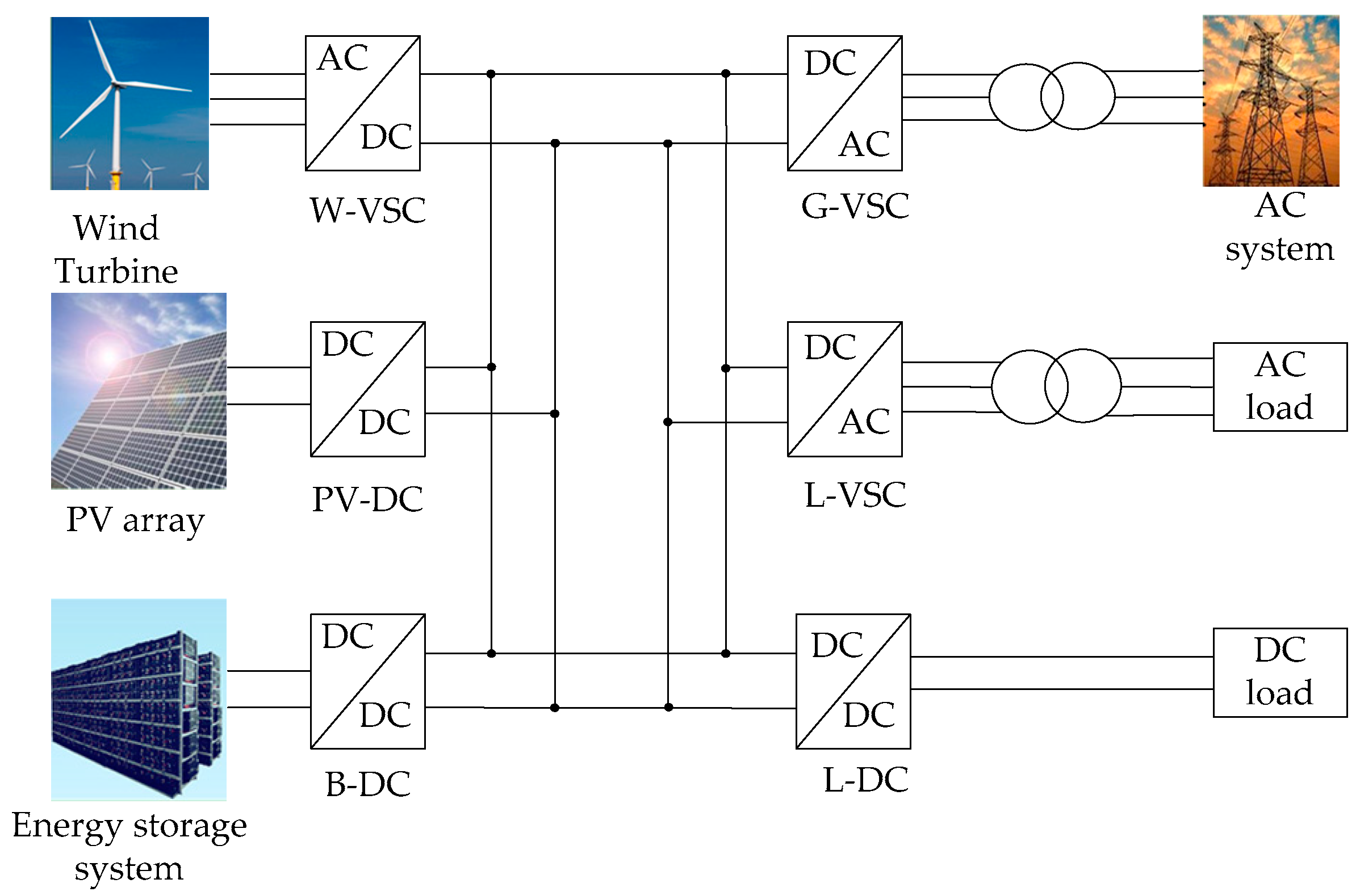
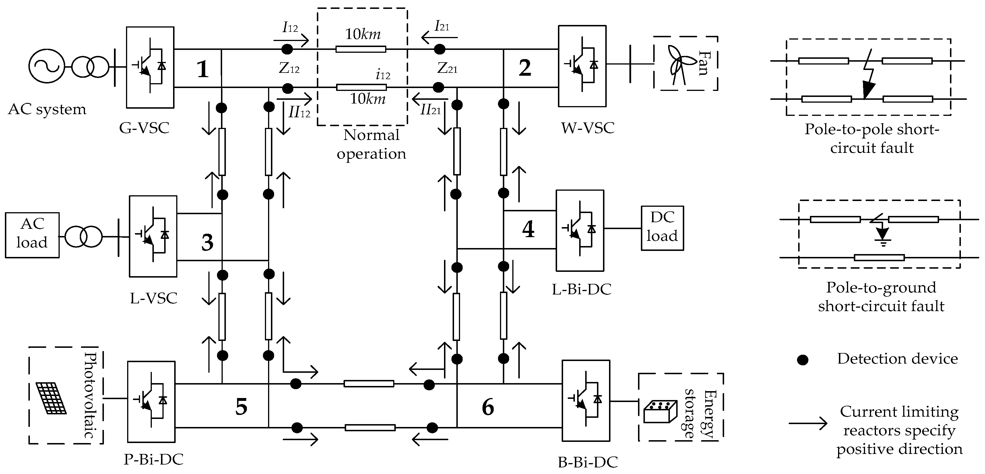
2.1. System Structure

The typical DC distribution system is mainly composed of new energy power generation units, energy storage units, load units, and network converters, as shown in Figure 1. The new energy power generation unit includes a wind power generation unit and a photovoltaic power generation unit. The load unit is divided into a DC load and an AC load according to the power supply, and the storage battery is used as the storage unit. Each unit in Figure 1 is connected to the common DC bus through inverters. The DC bus voltage has become a key indicator for measuring the stable operation of the distribution system. Under normal circumstances, in order to enhance economic efficiency, new energy power generation units such as wind turbines and photovoltaics should work in the condition of maximum power point tracking (MPPT). Under special circumstances, they can also be operated at reduced-power mode. According to the rated voltage, the DC load can be directly connected to the DC bus and can also be connected to the DC bus through a step-up or step-down chopper inverter L-DC. The AC load is connected to the DC bus through the voltage source converter (L-VSC). The storage unit is connected to the DC bus via a step-up chopper inverter B-DC, which can flow in both directions, and the B-DC is controlled by voltage and current in a double closed loop.

In various types of faults in DC distribution systems, the line fault occurs most frequently, and the instantaneous fault current reaches the peak within a few milliseconds, causing serious damage to the system. Therefore, higher requirements are put forward on fault location. Line faults include pole-to-pole short-circuit fault, pole-to-ground short-circuit fault, and disconnection fault. Considering that the probability and the degree of harm of disconnection fault are small, this paper mainly investigates fault location methods for pole-to-pole short-circuit faults and pole-to-ground short-circuit faults. The entire fault process can be divided into three phases: the capacitor discharge stage, the freewheeling phase of the diode, and the steady state phase under the action of the AC power supply [10]. For short-circuit faults, if the DC-side capacitor voltage drops below zero, there will be a three-phase short circuit on the AC side and a rapid overcurrent on the free-wheeling diode, which will seriously affect the safe operation of the AC system and burn-out the freewheeling diode. Therefore, in order to fully protect the DC lines, inverters, and AC systems, the quick protection action and DC circuit breaker tripping should occur before the DC capacitor voltage oscillates around zero crossing time. This prevents the three-phase short circuit condition on the AC side and the overcurrent diode from being subjected to a sudden overcurrent. So, this article mainly studies the capacitor discharge phase [4].

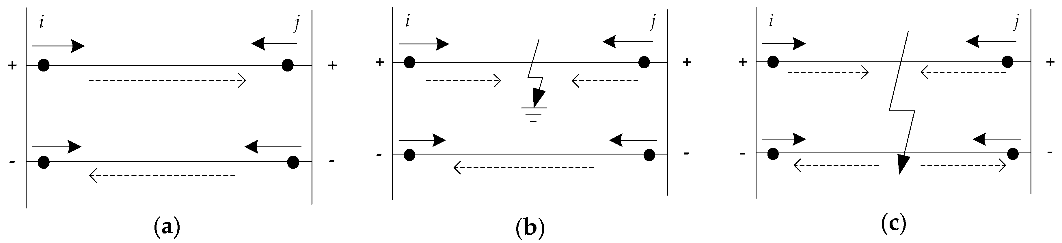
2.2. Mathematical Model of Pole-to-Pole Short-Circuit Fault

When the pole-to-pole short-circuit fault occurs, due to the self-protection function of the IGBT, the converter shuts instantaneously and the influence of the AC side current can be neglected. The current on the line is all derived from the discharge of the capacitor. Assume that the fault occurs in the line between the wind turbine (system 1) and the AC system (system 2). The equivalent circuit diagram at this stage is shown in Figure 2 [16].

In Figure 2, subscript 1 indicates the parameter that is close to system 1 with the fault point as the boundary. Subscript 2 indicates the parameter that is close to system 2 with the fault point as the boundary. C_i (I = 1, 2, the following i takes the same value) is the capacitance. V_dci is the voltage between the capacitor ends. R_i is the line resistance. Set the line resistance per unit length to r. Then R_i = r × D_i. L_i is the line inductance. Set the line inductance per unit length to l. Then L_i = l × D_i. I_i is the current flowing through the fault line. R_f is the transition resistance. D is the total length of the line.

According to the KVL theorem, the following formula can be obtained for system 1:

$$\{\begin{array}{l}{V}_{\mathrm{dc}1}=2I_1{R}_1+2L_1\frac{\mathrm{d}{I}_1}{\mathrm{d}t}+(I_1+I_2)R_f\hfill \\ I_1=C_1\frac{d{V}_{\mathrm{dc}1}}{dt}\hfill \end{array}$$

(1)

Similarly, the formula for system 2 is as follows:

$$\{\begin{array}{l}{V}_{\mathrm{dc}2}=2I_2{R}_2+2L_2\frac{\mathrm{d}{I}_2}{\mathrm{d}t}+(I_1+I_2)R_f\hfill \\ I_2=C_2\frac{d{V}_{\mathrm{dc}2}}{dt}\hfill \end{array}$$

(2)

In order to eliminate the influence of the transition resistance, solve Equations (1) and (2), then:

$$2L_2{C}_2\frac{d^2{V}_{\mathrm{dc}2}}{\mathrm{d}{t}^2}-2L_1{C}_1\frac{{\mathrm{d}}^2{V}_{\mathrm{dc}1}}{\mathrm{d}{t}^2}+2C_2{R}_2\frac{\mathrm{d}{V}_{\mathrm{dc}2}}{\mathrm{d}t}-2C_1{R}_1\frac{\mathrm{d}{V}_{\mathrm{dc}1}}{\mathrm{d}t}-V_{\mathrm{dc}2}+V_{\mathrm{dc}1}=0$$

(3)

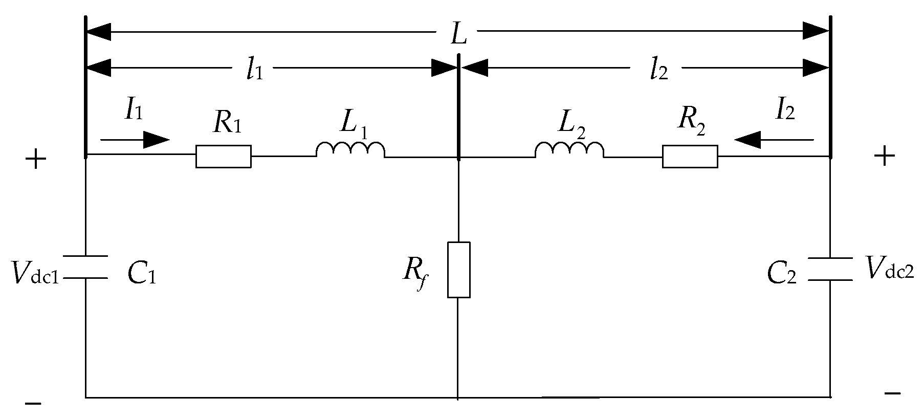
2.3. Mathematical Model of Pole-to-Ground Short-Circuit Fault

When a pole-to-ground short-circuit fault occurs in a DC power distribution system based on voltage source converters, the equivalent circuit diagram of the capacitance discharge phase is shown in Figure 3 [16].

The pole-to-ground short-circuit fault analysis process is the same as the pole-to-pole short-circuit fault. According to the KVL theorem, the following formula can be obtained for system 1:

$$\{\begin{array}{l}{V}_{\mathrm{dc}1}=I_1{R}_1+L_1\frac{\mathrm{d}{I}_1}{\mathrm{d}t}+(I_1+I_2)R_f\hfill \\ I_1=C_1\frac{d{V}_{\mathrm{dc}1}}{dt}\hfill \end{array}$$

(4)

Similarly, the formula for system 2 is as follows:

$$\{\begin{array}{l}{V}_{\mathrm{dc}2}=I_2{R}_2+L_2\frac{\mathrm{d}{I}_2}{\mathrm{d}t}+(I_1+I_2)R_f\hfill \\ I_2=C_2\frac{d{V}_{\mathrm{dc}2}}{dt}\hfill \end{array}$$

(5)

In order to eliminate the influence of the transition resistance, solve Equations (4) and (5), then:

$$L_2{C}_2\frac{d^2{V}_{\mathrm{dc}2}}{\mathrm{d}{t}^2}-L_1{C}_1\frac{{\mathrm{d}}^2{V}_{\mathrm{dc}1}}{\mathrm{d}{t}^2}+C_2{R}_2\frac{\mathrm{d}{V}_{\mathrm{dc}2}}{\mathrm{d}t}-C_1{R}_1\frac{\mathrm{d}{V}_{\mathrm{dc}1}}{\mathrm{d}t}-V_{\mathrm{dc}2}+V_{\mathrm{dc}1}=0$$

(6)

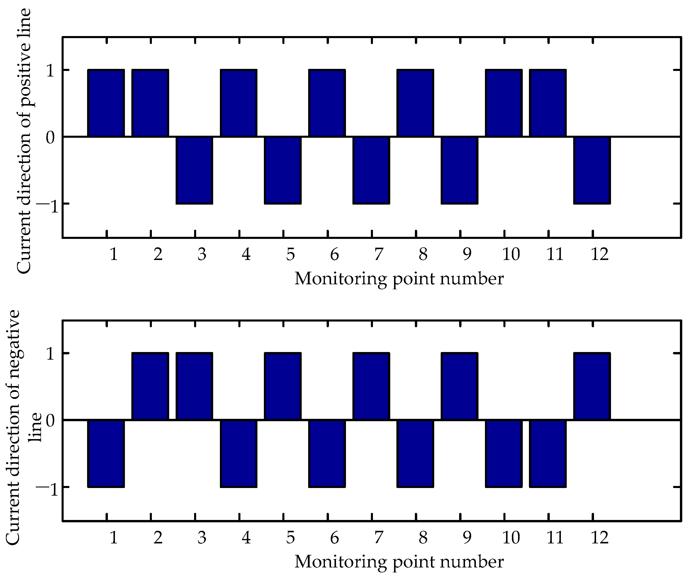
3. Fault Type Identification Algorithm Based on Graph Theory

3.1. The Basic Knowledge of Graph Theory

Definition 1.

A graph consists of several different vertices and edges connecting the different vertices [17].

The constituent elements of a graph are the points, often called vertices, and the edges, which are ordered pairs of vertices. If two vertices can be connected by an edge, the two vertices have adjacent relations. The chart can generally be shown as G = (V, E), where V is the set of all vertices. V = [v₁, v₂, ..., v_n]. E is a multiple subset of the Cartesian product. E = [e₁, e₂, ..., e_n]. Its elements are called directed edges or edges for short.

Definition 2.

Suppose G (G = (V, E)) to be a digraph with no margin. When V = [v₁, v₂, ..., v_n], the N × N matrix D (D = [d_ij]) is called the adjacency matrix of the G graph, denoted as D [G]. The adjacency matrix is a matrix representing the relationship between the vertices. Where,

$$d_{ij}=\{\begin{array}{c}0(v_i,v_j)\notin \mathit{E}\\ 1(v_i,v_j)\in \mathit{E}\end{array}$$

(7)

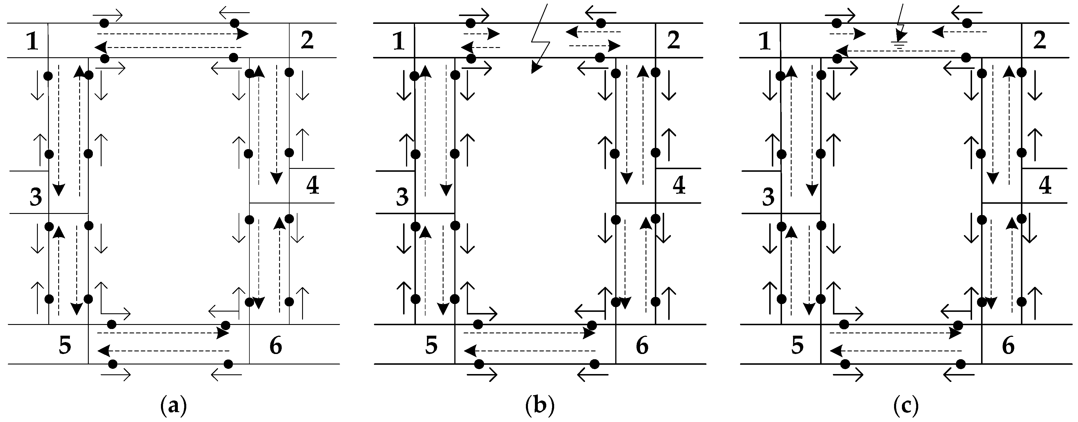
3.2. Directed Topology Description of a Distribution System

Regardless of the type of system structure, the system is composed of switches, overhead lines, and a variety of other devices. Thus, the network composition can be simplified, and the directional topology of the distribution system can be obtained.

According to Definition 1, the intersection of the distribution system lines can be seen as a vertex. Lines between vertices can be considered as directed edges, and the current flow on the feeder indicates the direction of the edge. Then, the distribution system can be regarded as a graph. The connection relationship between the vertex and feeder in the distribution system can be described by the definition of the graph, and the topology of the distribution system can be described by the adjacency matrix in Definition 2.

When a fault occurs, the direction of the current flowing through the distribution feeder changes immediately. Therefore, the feeder of the distribution system can be viewed as a directional edge. Assume that the number of nodes in the distribution system is n. The distribution system (hereafter referred to the system topology matrix) can be described by an n-order adjacency matrix D. If the direction of the edge is vertex i pointing to vertex j, the element d_ij = 1, in the matrix D. If the direction of the edge is vertex j pointing to vertex i, the element d_ij = −1, in the matrix D. The remaining elements are all zero. That is, the reference direction of the current transformer is defined as the vertex pointing to the line. According to the above principle, the initial value is set for the matrix D under normal operating conditions of the system.

In actual application, the determination of the current direction can be obtained through matching the current transformer and the ammeter, and the connection method is as shown in Figure 4. First, set initial values for elements in the matrix D based on normal operating conditions. In the figure, the primary coil has a leading end of L₁ and a trailing end of L₂. The first end of the secondary coil is K₁ and the end of the secondary coil is labeled K₂. The reference direction of the ammeter is expressed by the black arrow in Figure 4a, and the marker “*” indicates the same polarity end of the current transformer.

Figure 4a is a schematic diagram of the current flow in the current transformer under system normal operation. Since there is no major change in the primary current, no current is induced on the secondary side and the ammeter shows 0. The elements in the matrix D keep the original values at this time. When the current at the detection point changes, the primary current of the current transformer undergoes two processes. Firstly, the flow of I₁ from the L₁ terminal rapidly decreases to 0, then the direction of I₁ changes. Secondly, the current flows from the L₂ terminal, and the current value increases rapidly. The direction of current induced from the secondary side is shown in Figure 4b,c, respectively. In this case, the secondary current flow direction is opposite to the positive direction of the current meter, and the currents flowing through the current meter is negative. At this time, the elements in the matrix D are the opposite of the original values.

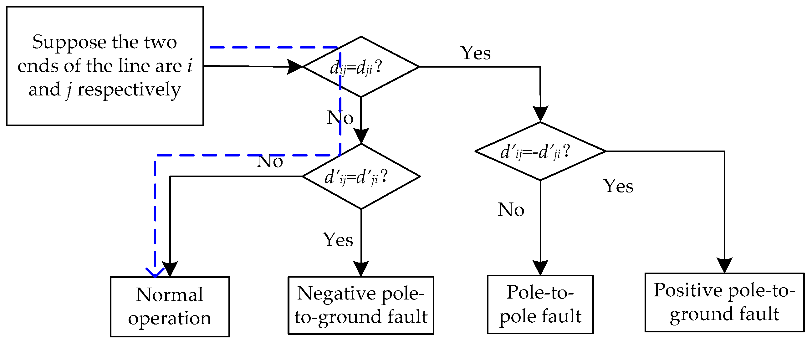
3.3. Fault Type Identification Algorithm

The system topological matrix formed by the current directions at both ends of the positive line is the matrix D. The system topological matrix formed by the current directions at both ends of the negative line is the matrix D′. When the system operates normally, the elements corresponding to the position of matrix D and matrix D′ are opposite each other. Two types of fault diagrams are shown in Figure 5, where i and j represent both ends of the same line. The specific process to identify the fault type is described below:

Normal operation. Recorded as (0,0). The two elements at the same position in matrices D and D′ are opposite to each other and are nonzero. From Figure 5a, it can be seen that d_ij = 1, d_ji = −1 in the matrix D, while d′_ji = 1, d′_ij = −1 in the matrix D′. The criterion is that, during normal operation, d_ij and d_ji are opposite to each other and ≠0. The relationship between d′_ji and d′_ij is the same.

Pole-to-ground short-circuit fault. Positive pole-to-ground short-circuit fault and negative pole-to-ground short-circuit fault are marked as (1,0) and (0,1), respectively. The two elements in the matrix where the matrix D or D′ represents the current directions of the fault occurrence lines are 1, and the other elements are not affected. From Figure 5b, we know that d_ij = d_ji = 1 in the matrix D and d′_ji = 1, d′_ij = −1 in the matrix D′. The criterion is that, when the positive line suffers a pole-to-ground short-circuit fault, d_ij = d_ji ≠ 0. d′_ji and d′_ij are opposite to each other and ≠0. When the negative line has a pole-to-ground short-circuit fault, d′_ij = d′_ji ≠ 0. d_ji and d_ij are opposite to each other and ≠0.

Pole-to-pole short-circuit fault. Recorded as (1,1). The two elements in matrix D are “1”, which indicates that the current directions at both ends of fault line constitute the vertex pointing to the line, and the two elements in matrix D′ are −1. In Figure 5c, it can be seen that d_ij = d_ji = 1 in the matrix D and d′_ji = d′_ij = −1 in the matrix D′. The criterion is: d_ij = d_ji ≠ 0 and d′_ji = d′_ij ≠ 0 in the fault line.

The short solid arrow represents the specified current positive direction, and the long dotted arrow represents the current flow.

Based on the above analysis, the algorithm flowchart of fault type identification is obtained in Figure 6. According to Figure 6, each pair of elements in the matrix D is traversed.

4. Fault Identification Method Based on Parameter Identification

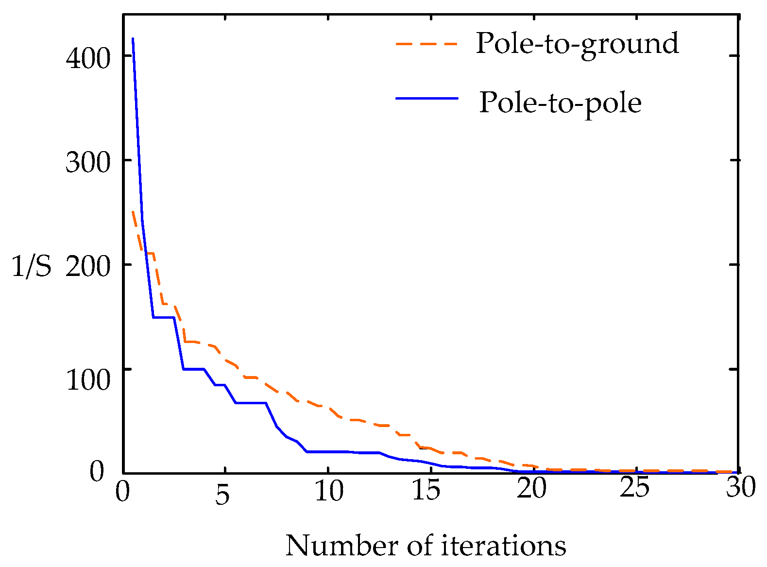
4.1. Application of GA in Parameter Identification

GA has a strong global search capability in solving the problem of parameter identification, and it uses selection, crossover, and mutation operators to search, avoiding the premature phenomenon in iterative processes [18]. The application steps of GA in programming problems are as follows:

• Population initialization operation. This step needs to determine the evolutionary generation, population size, crossover probability, mutation probability, and so on.
• Determination of fitness function. In the natural world, there is greater chance of survival for individuals with greater fitness, so it is necessary to transform the parameter identification problem into a fitness function. Individuals with a high degree of fitness are retained for the next generation of operations.
• Perform crossover and mutation operations on the remaining individuals.
• Diagnose whether the fitness value obtained and the last iteration meets the accuracy requirements. If it is satisfied, stop the iteration. Otherwise, continue to iterate until it reaches the optimal value. Then stop the iteration and output the result.

4.2. Differential Variable Extraction

When the sampling data on both sides are fully synchronized, it can be seen from Equations (3) and (6) that the values of R₁, R₂, L₁, and L₂ to be obtained and the voltage across the capacitor on both sides of the faulty line need to be sampled. For the acquisition of the differential quantities, this paper adopts the difference method to calculate the current rate of change. The sampling interval can be selected from 20 to 100 μs. In the formula, the first-order differential and second-order differential can be approximated by the backward difference, as shown in Equation (8):

$$\{\begin{array}{l}\frac{\mathrm{d}{V}_{\mathrm{dc}}}{\mathrm{d}t}=\frac{V_{\mathrm{dc}}(k)-V_{\mathrm{dc}}(k-2)}{2\Delta t}\hfill \\ \frac{{\mathrm{d}}^2{V}_{\mathrm{dc}}}{\mathrm{d}{t}^2}=\frac{V_{\mathrm{dc}}(k)-2V_{\mathrm{dc}}(k-1)+V_{\mathrm{dc}}(k-2)}{\Delta t^2}\hfill \end{array}$$

(8)

In the above formula, k is the sampling constant; V_dc (k), V_dc (k − 1), and V_dc (k − 2) are the current sampling values of the voltage, the previous sampling values and the sampling values before the previous sampling values, respectively. Δt is the sampling time interval.

4.3. Fault Location Principle

The unknowns in Equations (3) and (6) are R₁, R₂, L₁, and L₂, and the number of parameters to be identified is four. Since the values of these four quantities have a linear relationship with the fault location, the fault location can be achieved by solving the quantites. Discretize Equations (3) and (6) to obtain Equations (9) and (10):

$$\left[\begin{array}{l}-\frac{C_1}{\Delta t}{V}_{\mathrm{dc}1}(k)+\\ \frac{C_1}{\Delta t}{V}_{\mathrm{dc}1}(k-2)\end{array}\right]R_1+\left[\begin{array}{l}\frac{C_2}{\Delta t}{V}_{\mathrm{dc}2}(k)-\\ \frac{C_2}{\Delta t}{V}_{\mathrm{dc}2}(k-2)\end{array}\right]R_2+\left[\begin{array}{l}-\frac{2C_1}{\Delta t^2}{V}_{\mathrm{dc}1}(k)+\\ \frac{4C_1}{\Delta t^2}{V}_{\mathrm{dc}1}(k-1)-\\ \frac{2C_1}{\Delta t^2}{V}_{\mathrm{dc}1}(k-2)\end{array}\right]L_1+\left[\begin{array}{l}\frac{2C_2}{\Delta t^2}{V}_{\mathrm{dc}2}(k)-\\ \frac{4C_2}{\Delta t^2}{V}_{\mathrm{dc}2}(k-1)+\\ \frac{2C_2}{\Delta t^2}{V}_{\mathrm{dc}2}(k-2)\end{array}\right]L_2-V_{\mathrm{dc}}{}_2(k)+V_{\mathrm{dc}1}(k)=0$$

(9)

$$\left[\begin{array}{l}-\frac{C_1}{2\Delta t}{V}_{\mathrm{dc}1}(k)+\\ \frac{C_1}{2\Delta t}{V}_{\mathrm{dc}1}(k-2)\end{array}\right]R_1+\left[\begin{array}{l}\frac{C_2}{2\Delta t}{V}_{\mathrm{dc}2}(k)-\\ \frac{C_2}{2\Delta t}{V}_{\mathrm{dc}2}(k-2)\end{array}\right]R_2+\left[\begin{array}{l}-\frac{C_1}{\Delta t^2}{V}_{\mathrm{dc}1}(k)+\\ \frac{2C_1}{\Delta t^2}{V}_{\mathrm{dc}1}(k-1)-\\ \frac{C_1}{\Delta t^2}{V}_{\mathrm{dc}1}(k-2)\end{array}\right]L_1+\left[\begin{array}{l}\frac{C_2}{\Delta t^2}{V}_{\mathrm{dc}2}(k)-\\ \frac{2C_2}{\Delta t^2}{V}_{\mathrm{dc}2}(k-1)+\\ \frac{C_2}{\Delta t^2}{V}_{\mathrm{dc}2}(k-2)\end{array}\right]L_2-V_{\mathrm{dc}}{}_2(k)+V_{\mathrm{dc}1}(k)=0$$

(10)

Only five sets of voltage values are required to solve the above equations, and the sampling information is redundant. In order to avoid the occurrence of distance-measuring error due to identification error of the individual sample points, GA is used to optimize the parameter identification. The fitness function S (R₁, R₂, L₁, L₂) is expressed as follows:

$$S(R_1,R_2,L_1,L_2)=\frac{1}{{\displaystyle \sum _{k=1}^{N-1}{f}_k^2(R_1,R_2,L_1,L_2)}}$$

(11)

Among them, the function f represents Equations (8) and (9). Since the right side of the equals sign is 0, the smaller the denominator in Equation (10) is, the better the individual is. Therefore, the fitness can also be stronger. The algorithm flow chart is shown in Figure 7:

5. Simulation Verification

5.1. Simulation Results for Fault Type Identification

5.1.1. Parameter Settings

A benchmark system of a six-terminal system is established, and the system includes an AC main grid connection, wind turbine, AC and DC loads, energy storage systems, and photovoltaic generation. The length of the line between each end is 10 km. The benchmark system is shown in Figure 8. In Figure 8, the current flowing through the DC inductor on the positive line is denoted by I_mk (m, k denote that the current flows from the m end to the k end in the positive direction). Similarly, the current on a negative line is represented as II_mk. The detection device on the positive line is denoted by Z_mk (m, k denote that the current flows from the m end to the k end in the positive direction). Similarly, the current on a negative line is represented as Z’_mk. The simulation time is 0.4 s, the fault occurrence time is 0.15 s.

The grounding method of the DC system capacitor is divided into four types: split capacitor neutral point grounding, positive line grounding, negative line grounding, and un-grounding. Among them, the positive line grounding and the negative line grounding make the non-grounding pole withstand all the DC voltage, and have a high requirement for the insulation level of the line. When not grounded, large high-frequency harmonic currents flow in the DC line, causing large interference to the communication line, and generating a large high-frequency AC voltage in the line, which results in a high-frequency AC drift component at the midpoint of the DC capacitor [19]. Taking the above factors into account, the DC capacitors of G-VSC, W-VSC, P-Bi-DC, and B-Bi-DC shown in Figure 8 are directly grounded, and the DC-side capacitors of L-VSC and L-Bi-DC are un-grounding.

The simulation parameters are shown in

Table 1. Parameters of the model.

Parameters	Value
DC bus voltage	500 V
Converter DC side capacitance	2 mF
Wind power unit	20 kW/220 V Permanent Magnet Wind Turbine Rated wind speed is 12 m/s Rated speed is 75 r/min
Rated power of G-VSC	20 kW
Battery rated power	20 kW
Load unit rated power	20 kW
Line resistance	0.0139 Ω/km
Line inductance	0.159 mH/km
Line length	10 km
Sampling frequency	25 μs

.

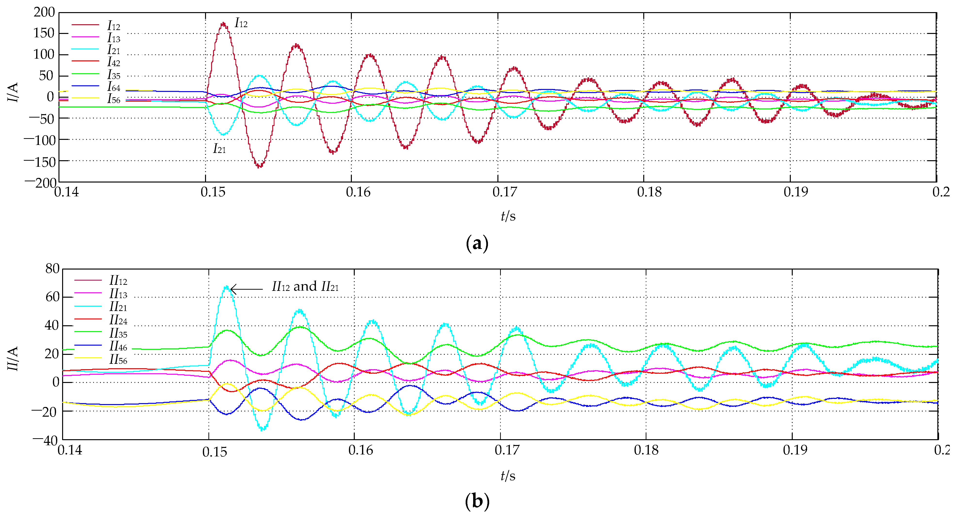
5.1.2. Results Analysis

To illustrate the effectiveness of the proposed protection, a fault is set on the line between apex 1 and 2. The three cases of normal operation, pole-to-pole short-circuit fault, and pole-to-ground short-circuit fault are simulated. For the pole-to-pole short-circuit faults and pole-to-ground short-circuit faults, the fault is set at the midpoint of the line. The current flow of the system in the three cases is shown in Figure 9. The dashed lines in the figure indicate the actual current flow.

Normal Operation

The current flow during the normal operation of the system is as shown in Figure 9a. The current direction is detected based on the configuration of current transformers and ammeters at both ends of each side. The current flow at the monitoring point is shown in Figure 10.

From Figure 10, the figures and their representative monitoring devices are shown in

Table 2. The figures and their representative monitoring devices.

Number	1	2	3	4	5	6	7	8	9	10	11	12
Monitoring point-positive line	Z12	Z21	Z13	Z31	Z24	Z42	Z35	Z53	Z46	Z64	Z56	Z65
Monitoring point-negative line	Z’12	Z’21	Z’13	Z’31	Z’24	Z’42	Z’35	Z’53	Z’46	Z’64	Z’56	Z’65

.

Set the initial value for the system topology matrix D according to the normal operation. Take the positive line as an example. As can be seen from Figure 10, d₁₂ = d₁₃ = d₂₄ = d₅₃ = d₅₆ = d₆₄ = 1, d₂₁ = d₃₁ = d₃₅ = d₄₂ = d₄₆ = d₆₅ = −1, and the remaining elements are all zero. The negative line analysis process is the same. The 6-dimensional system topology matrices D and D′ can be represented as follows.

$$\begin{array}{cc}\mathit{D}=\left[\begin{array}{cccccc}0& 1& 1& 0& 0& 0\\ -1& 0& 0& 1& 0& 0\\ -1& 0& 0& 0& -1& 0\\ 0& -1& 0& 0& -1& 0\\ 0& 0& 1& 0& 0& 1\\ 0& 0& 0& 1& -1& 0\end{array}\right]& {\mathit{D}}^{\prime }=\left[\begin{array}{cccccc}0& -1& -1& 0& 0& 0\\ 1& 0& 0& -1& 0& 0\\ 1& 0& 0& 0& 1& 0\\ 0& 1& 0& 0& 1& 0\\ 0& 0& -1& 0& 0& -1\\ 0& 0& 0& -1& 1& 0\end{array}\right]\end{array}$$

According to Figure 6, the process is shown in Figure 11, which can output the result “This system is operating normally.”

Pole-to-Pole Short-Circuit Fault

The system during the pole-to-pole short-circuit fault is shown in Figure 9b. The current waveform under pole-to-pole short-circuit fault conditions is shown in Figure 12. The current flow at the monitoring point is shown in Figure 13.

Comparing Figure 10 with Figure 13, the elements in D and D′ are refreshed. The elements that change the direction of the current are: d₂₁, d₁₃, d₃₁, d₂₄, d₄₂, $d_{21}^{\prime }$, $d_{13}^{\prime }$, $d_{31}^{\prime }$, $d_{24}^{\prime }$, $d_{42}^{\prime }$, and the rest of the elements remain unchanged. The 6-dimensional system topology matrices D and D′ can be represented as follows.

$$\begin{array}{cc}\mathit{D}=\left[\begin{array}{cccccc}0& 1& -1& 0& 0& 0\\ 1& 0& 0& -1& 0& 0\\ 1& 0& 0& 0& -1& 0\\ 0& 1& 0& 0& -1& 0\\ 0& 0& 1& 0& 0& 1\\ 0& 0& 0& 1& -1& 0\end{array}\right]& {\mathit{D}}^{\prime }=\left[\begin{array}{cccccc}0& -1& 1& 0& 0& 0\\ -1& 0& 0& 1& 0& 0\\ -1& 0& 0& 0& 1& 0\\ 0& -1& 0& 0& 1& 0\\ 0& 0& -1& 0& 0& -1\\ 0& 0& 0& -1& 1& 0\end{array}\right]\end{array}$$

According to Figure 6, Figure 14 shows the fault type judgment process of the line between vertex 1 and vertex 2. The output result is “The line between vertices 1 and 2 of this system has a pole-to-pole short-circuit fault”.

Positive Pole-to-Ground Short-Circuit Fault

The current flow during the pole-to-ground short-circuit fault of the system is shown in Figure 9c. The current waveform under pole-to-ground short-circuit fault conditions is shown in Figure 15. The current flow at the monitoring point is shown in Figure 16.

Comparing Figure 10 with Figure 16, the elements in D and D′ are refreshed. The elements that change the direction of the current are: d₂₁, d₁₃, d₃₁, d₂₄, d₄₂, $d_{21}^{\prime }$, $d_{13}^{\prime }$, $d_{31}^{\prime }$, $d_{24}^{\prime }$, $d_{42}^{\prime }$, and the rest of the elements remain unchanged. The 6-dimensional system topology matrices D and D′ can be represented as follows.

$$\begin{array}{cc}\mathit{D}=\left[\begin{array}{cccccc}0& 1& -1& 0& 0& 0\\ 1& 0& 0& -1& 0& 0\\ 1& 0& 0& 0& -1& 0\\ 0& 1& 0& 0& -1& 0\\ 0& 0& 1& 0& 0& 1\\ 0& 0& 0& 1& -1& 0\end{array}\right]& {\mathit{D}}^{\prime }=\left[\begin{array}{cccccc}0& -1& 1& 0& 0& 0\\ 1& 0& 0& 1& 0& 0\\ -1& 0& 0& 0& 1& 0\\ 0& -1& 0& 0& 1& 0\\ 0& 0& -1& 0& 0& -1\\ 0& 0& 0& -1& 1& 0\end{array}\right]\end{array}$$

According to Figure 6, Figure 17 shows the fault type judgment process of the line between vertex 1 and vertex 2. The output result is “The line between vertices 1 and 2 of this system has an positive pole-to-ground short-circuit fault”.

5.2. Fault Location Results

5.2.1. Parameter Settings

There are 4 parameters to be identified, so the search dimension is 4. The range of the parameters is as follows: R₁ and R₂ have a range of 0~r × D. L₁ and L₂ have a range of 0~l × D. The population size is generally 5–10 times the dimension. The population size is taken as 20 because the fault location requires a high speed of the algorithm. The sampling of the voltage needs to take 22 points after the failure. The crossover probability is 0.7. The mutation probability is 0.01. The generation gap is 0.95. To ensure the quick action of protection, the largest genetic generation is taken as 30 times. The values of the parameters are shown in

Table 3. The initial population values of the genetic algorithm.

The range of R1	0~r × D
Range of R2	0~r × D
Range of L1	0~l × D
Range of L2	0~l × D
Search dimension	4
Population size	20
Crossover probability	0.7
Mutation probability	0.01
Generation gap	0.95
Largest genetic generation	30

. The initial population determination process is as follows: Firstly, the 22 groups of voltage values after the occurrence of the fault are sampled. Secondly, according to Equations (9) and (10), the number of effective equations is 20 groups. With 4 unknowns, 4 equations can solve a set of parameter values. A total of $C_{20}^4$ initial populations can be calculated. Thirdly, randomly choose 20 groups of parameter values to form the initial population.

5.2.2. Results Analysis

Pole-to-ground short-circuit fault conditions and pole-to-pole short-circuit fault conditions are simulated separately. Observe the value of 1/S (${\displaystyle \sum _{k=1}^{N-1}{f}_k^2(R_1,R_2,L_1,L_2)}$) as the number of iterations increases, as shown in the Figure 18. In the figure, the case where the transition resistance is 10 Ω and the actual positioning distance is 5 km is taken as an example. At the beginning of the iteration, the objective function of the inter-pole short-circuit fault is significantly larger than the ground fault, but the objective function between the poles decreases rapidly. On the whole, the objective function of the inter-pole short-circuit fault is smaller than the ground fault, and the final identification accuracy is also higher. It can be seen that in the 20th iteration, for the pole-to-pole short-circuit fault and the pole-to-ground fault, the value of 1/S converges, and the convergence is good while ensuring the convergence speed.

In order to judge the accuracy of parameter identification, curve fitting is needed for Equations (9) and (10) and it is written as a function form such as Equations (12) and (13). In the case of a pole-to-pole short-circuit fault in the system, the transition resistance is 10 Ω, and the actual positioning distance is 5 km. The obtained identification result is brought into Equation (12), and the fitting result is obtained as shown in Figure 19, the abscissa represents time, and the ordinate represents the value of the function y.

$$y_1(k)=\left[\begin{array}{l}-\frac{C_1}{\Delta t}{V}_{\mathrm{dc}1}(k)+\\ \frac{C_1}{\Delta t}{V}_{\mathrm{dc}1}(k-2)\end{array}\right]R_1+\left[\begin{array}{l}\frac{C_2}{\Delta t}{V}_{\mathrm{dc}2}(k)-\\ \frac{C_2}{\Delta t}{V}_{\mathrm{dc}2}(k-2)\end{array}\right]R_2+\left[\begin{array}{l}-\frac{2C_1}{\Delta t^2}{V}_{\mathrm{dc}1}(k)+\\ \frac{4C_1}{\Delta t^2}{V}_{\mathrm{dc}1}(k-1)-\\ \frac{2C_1}{\Delta t^2}{V}_{\mathrm{dc}1}(k-2)\end{array}\right]L_1+\left[\begin{array}{l}\frac{2C_2}{\Delta t^2}{V}_{\mathrm{dc}2}(k)-\\ \frac{4C_2}{\Delta t^2}{V}_{\mathrm{dc}2}(k-1)+\\ \frac{2C_2}{\Delta t^2}{V}_{\mathrm{dc}2}(k-2)\end{array}\right]L_2-V_{\mathrm{dc}}{}_2(k)+V_{\mathrm{dc}1}(k)$$

(12)

$$y_2(k)=\left[\begin{array}{l}-\frac{C_1}{2\Delta t}{V}_{\mathrm{dc}1}(k)+\\ \frac{C_1}{2\Delta t}{V}_{\mathrm{dc}1}(k-2)\end{array}\right]R_1+\left[\begin{array}{l}\frac{C_2}{2\Delta t}{V}_{\mathrm{dc}2}(k)-\\ \frac{C_2}{2\Delta t}{V}_{\mathrm{dc}2}(k-2\end{array}\right]R_2+\left[\begin{array}{l}-\frac{C_1}{\Delta t^2}{V}_{\mathrm{dc}1}(k)+\\ \frac{2C_1}{\Delta t^2}{V}_{\mathrm{dc}1}(k-1)-\\ \frac{C_1}{\Delta t^2}{V}_{\mathrm{dc}1}(k-2)\end{array}\right]L_1+\left[\begin{array}{l}\frac{C_2}{\Delta t^2}{V}_{\mathrm{dc}2}(k)-\\ \frac{2C_2}{\Delta t^2}{V}_{\mathrm{dc}2}(k-1)+\\ \frac{C_2}{\Delta t^2}{V}_{\mathrm{dc}2}(k-2)\end{array}\right]L_2-V_{\mathrm{dc}}{}_2(k)+V_{\mathrm{dc}1}(k)$$

(13)

The simulation data and the fitting curve are basically coincident, indicating that the identification result is good.

To estimate the fit error, the variable y is introduced. The formula of y is expressed as (14). y represents the average fitting error at each moment in each case. The value of j depends on the type of fault. When the fault type is a pole-to-pole short-circuit fault, j = 1; otherwise, j = 2.

$$y=\frac{{\displaystyle \sum _{k=1}^{20}{y}_j(k)}}{20}(j=1\mathrm{or}2)$$

(14)

Simulations and curve fitting were performed for 18 cases (see Table 3 for code representation), and Figure 20 was obtained. The abscissa represents 18 cases, and the ordinate represents the value of y.

It can be seen from Figure 20 that the average y of each time corresponding to each fault condition is between [−0.2–0.2], and the error is very small, giving the final positioning result, as shown in

Table 4. Simulation results.

Fault Type	Transition Resistance	Code	Actual Value	Targeting Value	The Error
Pole-to-pole short-circuit fault	0 Ω	1	1 km	1.0231 km	0.3100%
		2	5 km	4.9938 km	0.1240%
		3	7 km	7.0297 km	0.4243%
	10 Ω	4	1 km	0.9810 km	0.1900%
		5	5 km	5.0102 km	0.2040%
		6	7 km	6.9984 km	0.0229%
	50 Ω	7	1 km	1.0333 km	0.3300%
		8	5 km	5.0014 km	0.0280%
		9	7 km	6.9969 km	0.0443%
Pole-to-ground short-circuit fault	0 Ω	10	1 km	1.0072 km	0.7200%
		11	5 km	5.0100 km	0.2000%
		12	7 km	7.0003 km	0.0043%
	10 Ω	13	1 km	0.9922 km	0.7800%
		14	5 km	4.8991 km	0.2180%
		15	7 km	6.9893 km	0.1529%
	50 Ω	16	1 km	0.9918 km	0.8200%
		17	5 km	5.0027 km	0.0540%
		18	7 km	6.9931 km	0.0986%

:

According to the data in the table, no matter what position the fault occurs in, the error is below 1%. This method has a high location accuracy and wide application range. As can be seen from the data, this method is not affected by the transition resistance and has a strong robustness.

6. Conclusions

This paper transforms the fault location problem into a parameter identification problem. Through simulation verification, the following conclusions are drawn: For fault type identification, the fault type identification algorithm based on graph theory is applicable to various topologies and fault types, and the recognition result is accurate. This method forms a system topology matrix. When the logical elements are determined, the running states are represented by “0”, “1”, and “−1”. The sparsity of the matrix is very strong and the operation speed is fast. The mathematical model of the established fault stage eliminates the influence of the transition resistance. The simulation verification also shows that this positioning method has strong resistance to transition resistance. The GA algorithm has a strong global search capability, which ensures the positioning accuracy of the algorithm and the error is below 1%. It excludes the erroneous sampling information in the sampling process and has a strong robustness.

References

1. Vahedi, H.; Al-Haddad, K. Real-Time implementation of a packed U-Cell seven-Level inverter with low switching frequency voltage regulator. IEEE Trans. Power Electron. 2016, 31, 5967–5973. [Google Scholar] [CrossRef]
2. Lee, S.W.; Cho, B.H. Master–Slave based hierarchical control for a small power DC-distributed microgrid system with a storage device. Energies 2016, 9, 880. [Google Scholar] [CrossRef]
3. Liu, J.; Tai, N.; Fan, C.; Chen, S. A hybrid current-limiting circuit for DC line fault in multi-terminal VSC-HVDC system. IEEE Trans. Power Electron. 2017, 64, 5595–5607. [Google Scholar]
4. Li, B.; He, J. DC fault analysis and current limiting technique for VSC-based DC distribution system. Proc. CSEE 2015, 35, 3026–3036. [Google Scholar]
5. Xue, S.M.; Liu, C.; Sciubba, E. Line-to-Line fault analysis and location in a VSC-based Low-Voltage DC distribution network. Energies 2018, 11, 536. [Google Scholar]
6. Tang, L.; Boon-Teck, O. Locating and isolating DC faults in multi-terminal DC systems. IEEE Trans. Power Deliv. 2007, 22, 1877–1884. [Google Scholar] [CrossRef]
7. Park, J.D.; Candelaria, J.; Ma, L.; Dunn, K. DC ring-bus microgrid fault protection and identification of fault location. IEEE Trans. Power Deliv. 2013, 28, 2574–2584. [Google Scholar] [CrossRef]
8. Baran, M.E.; Mahajan, N.R. Overcurrent protection on voltage-source-converter-based multi-terminal DC distribution systems. IEEE Trans. Power Deliv. 2007, 22, 406–412. [Google Scholar] [CrossRef]
9. Cheng, J.; Guan, M.; Tang, L.; Huang, H.; Chen, X.; Xie, J. Paralleled multi-terminal DC transmission line fault locating method based on travelling wave. Let Gener. Transm. Distrib. 2014, 8, 2092–2101. [Google Scholar] [CrossRef]
10. He, Z.; Liao, K.; Li, X.; Lin, S.; Yang, J.; Mai, R. Natural frequency-based Line fault location in HVDC Lines. IEEE Trans. Power Deliv. 2014, 29, 851–859. [Google Scholar] [CrossRef]
11. Zhang, S.; Zou, G.; Huang, Q.; Gao, H. A traveling-wave-based fault location scheme for MMC-based multi-terminal DC grids. Energies 2018, 11, 401. [Google Scholar] [CrossRef]
12. Zhang, X.; Tai, N.; Wang, Y.; Liu, J. EMTR-based fault location for DC line in VSC-MTDC system using high-frequency currents. Let Gener. Transm. Distrib. 2017, 11, 2499–2507. [Google Scholar] [CrossRef]
13. Li, M.; Jia, K.; Bi, T.; Yang, Q. Sixth harmonic-based fault location for VSC-DC distribution systems. LET Gener. Transm. Distrib. 2017, 11, 3485–3490. [Google Scholar] [CrossRef]
14. Gao, S.; Sun, J.; Song, G.; Zhang, J.; Jiao, Z. Fault location method for HVDC transmission lines on the basis of the distributed parameter model. Proc. CSEE 2010, 30, 75–80. [Google Scholar]
15. Cai, X.; Song, G.; Gao, S.; Suonan, J.; Li, G. A novel fault-location method for VSC-HVDC transmission lines based on natural frequency of current. Proc. CSEE 2011, 31, 112–119. [Google Scholar]
16. Yang, J.; Fletcher, J.F.; O’Reilly, J. Short-circuit and ground fault analyses and location in VSC-based DC network cables. IEEE Trans. Power Electron. 2012, 59, 3827–3837. [Google Scholar]
17. Steven, D.A.F.; Patrick, J.N.; Stuart, J.G.; Paul, C.; Graeme, M.B. Optimizing the roles of unit and non-unit protection methods within DC microgrids. IEEE Trans. Smart Grid 2012, 3, 2079–2087. [Google Scholar]
18. Hussein, K.H.; Mota, I. Maximum photovoltaic power tracking: An algorithm for rapidly changing atmospheric conditions. IEE Proc. Gener. Transm. Distrib. 1995, 142, 59–64. [Google Scholar] [CrossRef]
19. Guan, M.; Xu, Z. DC side grounding methodology for a Two-level VSC HVDC system. Automat. Electr. Power Syst. 2009, 33, 55–60. [Google Scholar]
Figure 1. Typical structure of DC distribution systems.
Energies 11 01983 g001
Figure 2. Equivalent circuit diagram of capacitance discharge phase under pole-to-pole short-circuit fault.
Energies 11 01983 g002
Figure 3. Equivalent circuit diagram of capacitance discharge in pole-to-ground short-circuit fault.
Energies 11 01983 g003
Figure 4. Current direction acquisition diagram: (a) Normal operation; (b) I1 decreases rapidly; (c) I1 increases rapidly.
Energies 11 01983 g004
Figure 5. Fault-type diagram: (a) Normal operation; (b) Pole-to-ground short-circuit short-circuit fault; (c) Pole-to-pole short-circuit fault.
Energies 11 01983 g005
Figure 6. The algorithm flowchart of fault-type identification.
Energies 11 01983 g006
Figure 7. Algorithm flowchart.
Energies 11 01983 g007
Figure 8. System simulation diagram.
Energies 11 01983 g008
Figure 9. The current flow of the system under: (a) Normal operation; (b) Pole-to-pole short-circuit fault; (c) Pole-to-ground short-circuit fault.
Energies 11 01983 g009
Figure 10. The current flow of monitoring point during normal operation: (a) Positive line; (b) Negative line.
Energies 11 01983 g010
Figure 11. The algorithm flowchart under normal operation.
Energies 11 01983 g011
Figure 12. Pole-to-pole short-circuit fault condition: (a) Positive line current conditions; (b) Negative line current conditions.
Energies 11 01983 g012aEnergies 11 01983 g012b
Figure 13. The current flow of monitoring point during pole-to-pole short-circuit fault: (a) Positive line; (b) Negative line.
Energies 11 01983 g013
Figure 14. The algorithm flowchart under pole-to-pole short-circuit fault.
Energies 11 01983 g014
Figure 15. Pole-to-ground short-circuit fault condition: (a) Positive line current conditions; (b) Negative line current conditions.
Energies 11 01983 g015
Figure 16. The current flow of monitoring points during pole-to-ground short-circuit fault: (a) Positive line; (b) Negative line.
Energies 11 01983 g016
Figure 17. The algorithm flowchart under positive pole-to-ground short-circuit fault.
Energies 11 01983 g017
Figure 18. The relationship between the value of 1/S and the number of iterations.
Energies 11 01983 g018
Figure 19. Curve fitting results.
Energies 11 01983 g019
Figure 20. Eighteen kinds of fault condition fitting results.
Energies 11 01983 g020