1. Introduction
Renewable photovoltaic (PV) generation systems represent an attractive and viable alternative of electrical energy supply to decrease the environmental contamination and the global warming effect produced by the consumption of fossil fuels. The PV installations have been steadily growing over recent decades. At present, a considerable number of PV generation plants are connected to power networks or to supply isolated electrical loads [
1].
The dynamic performance of these PV generation systems is important for the planning, design, and operation of power networks where they are connected [
2,
3]. This work mainly focuses in a time domain (TD) framework for the representation of these interconnected PV generation system working under dynamic and periodic steady state operation conditions [
4].
Reported technical problems and limitations of PV generation are its variability, intermittency, and adverse power quality effects, such as harmonic distortion, voltage, and frequency variations [
5]. These problems can be analysed with the proposed TD methodology. The TD solution can be applied to take adequate control decisions, e.g., to regulate the power generation and the energy conversion process or to enhance the electrical network stability [
6,
7,
8].
The extrapolation to the limit cycle and Poincare map approach [
9] has been applied to quickly obtain the periodic steady state of electrical systems [
10,
11]. The proposed methodology extends this application to interconnected microgrids with PV sources, taking into account the energy conversion system through power electronic components, such as transistors, MOSFETs and IGBTs. This conversion process requires the commutation of these electronic devices at an adjustable or controllable frequency and needs an adequate time step during the TD solution process [
12]. Among the several methods reported in [
9], the Numerical Differentiation (ND) approach is known to have a relatively simple formulation and good precision characteristics. Besides, the ND method is numerically robust and it has good convergence properties [
13]. Therefore, in this contribution, it is used to speed-up the periodic steady state solution of the microgrid with interconnected PV generation, and to reduce the execution time and the computational effort required to obtain the periodic steady state solution in TD.
The cubic spline interpolation (CSI) is a technique that has been applied to accurately estimate a new point between known data with smaller error that the obtained by using square or linear interpolation [
14,
15]. The application of the cubic splines is proposed to adjust the number of points per cycle needed to represent the periodic steady state waveform. The CSI approach enhances the ND response with a time step reduction, thus avoiding a large computational effort. The CSI technique obtains new solution points, adjusted with a smaller error.
This contribution presents an efficient TD solution process to obtain the periodic steady state of microgrids with PV generation sources. This process incorporates fast and precise mathematical and numerical tools such as Newton Raphson (NR), trapezoidal rule (TR), DN, and CSI, respectively. The proposed TD methodology can be used to assess stability [
16,
17], power quality [
18,
19,
20], dynamic and periodic steady state operation, fault and transient conditions, among other issues, of microgrids with PV sources [
21].
The rest of the paper is organized as follows:
Section 2 deals with the microgrid description, its modelling and the interconnection of PV systems;
Section 3 reviews the ND method based on the Poincare map and the extrapolation to the limit cycle concepts;
Section 4 explains the CSI method to adjust the number of time steps per cycle and to define the time step to be used during the electrical system solution;
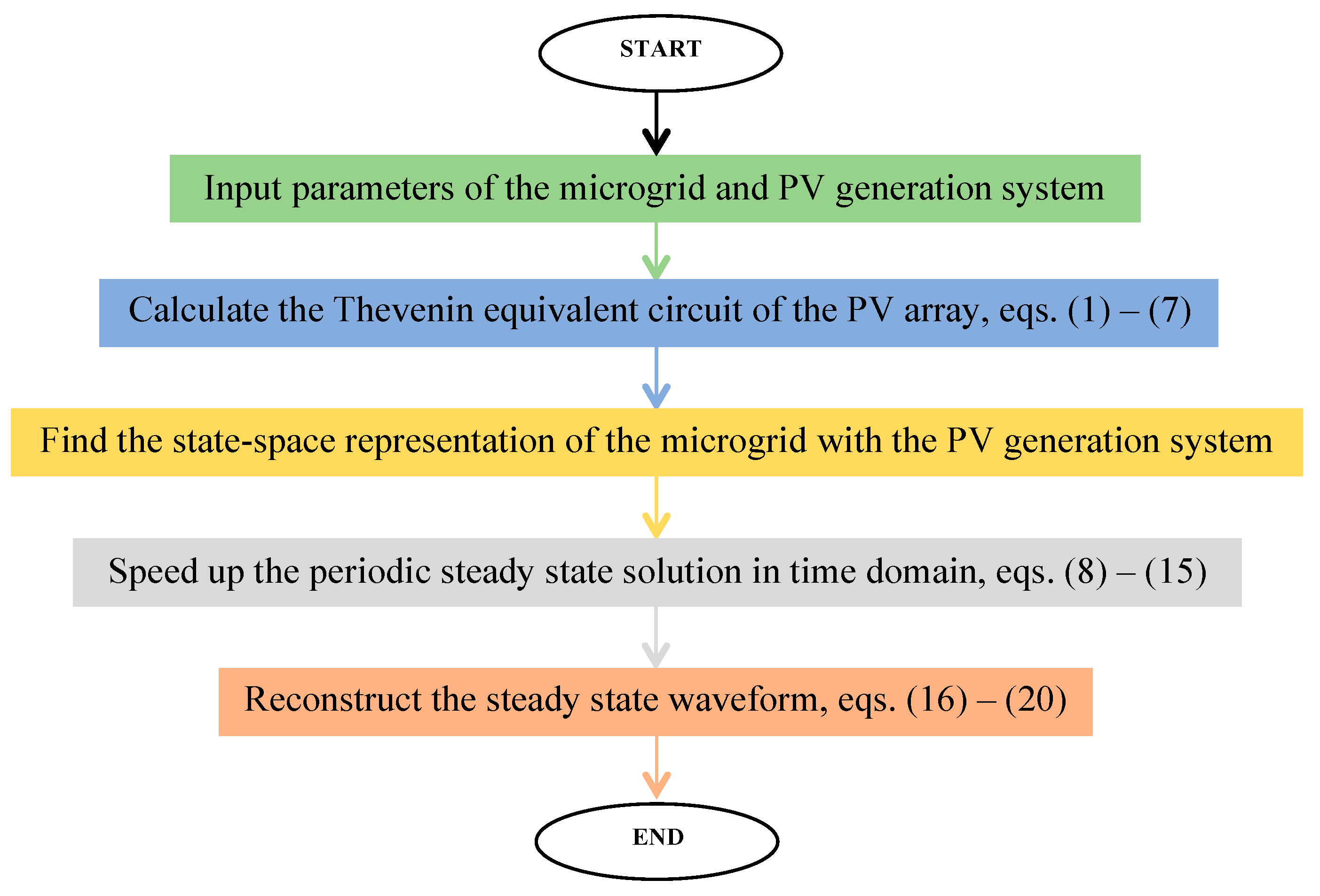
Section 5 details a flowchart of the solution procedure;
Section 6 reports the practical application of the methodology through a test case and limitations of the microgrid modelling;
Section 7 draws the main conclusions of this research work.
2. System Description and Modelling
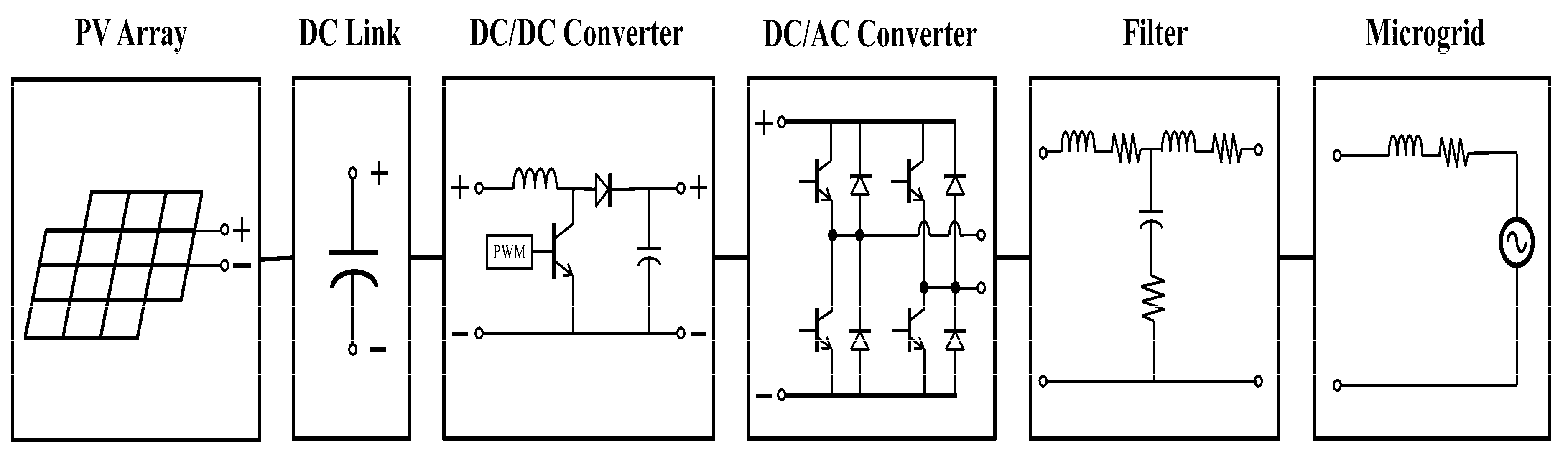
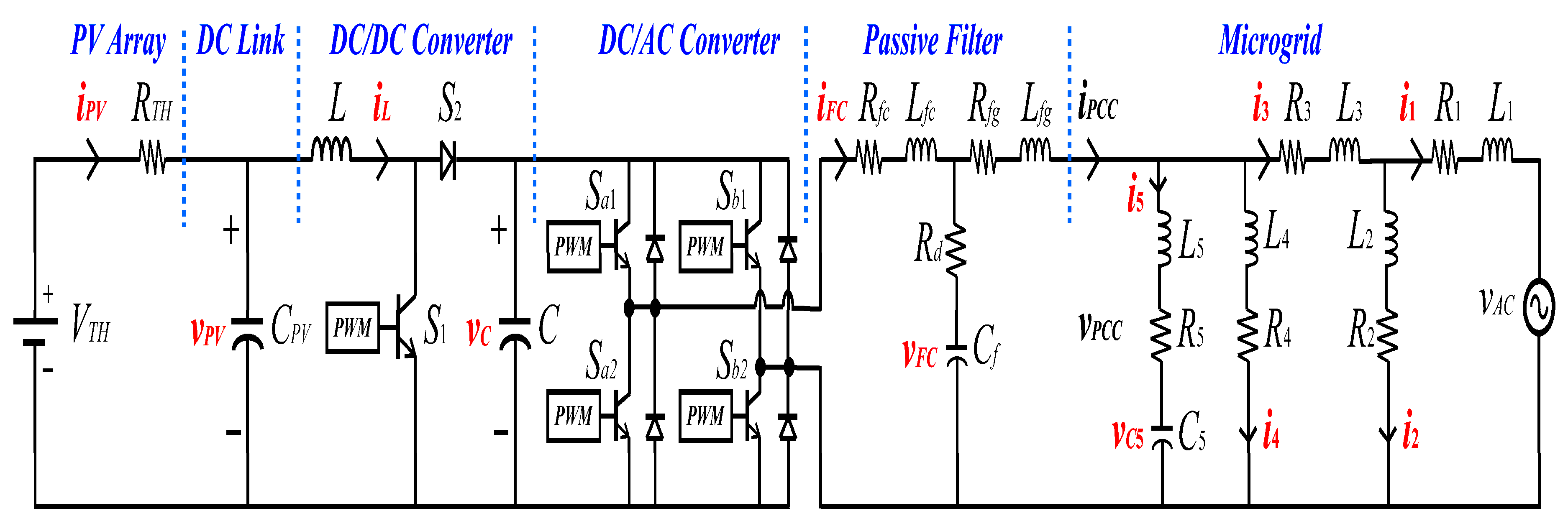
Figure 1 shows the configuration of a single-phase grid-connected PV generation system. It contains a PV array, a capacitor link, a DC/DC converter, a DC/AC converter, a filter, and a utility grid [
12].
The capacitor link is connected to the output of the PV array to decouple the AC-system dynamics from the PV array. The DC/DC converter is used to maintain an adequate voltage level and for maximum power point tracking (MPPT) of the generation system [
22]. The DC/AC converter is used to obtain AC power. Finally, the filter is used to mitigate the total harmonic distortion (THD) at the point of common coupling (PCC).
2.1. PV Array Model
Typically, a single PV cell generates an electrical power of about 1 to 3 W [
23]. To increase the power, several PV cells are connected in the appropriate series-parallel combination to form larger capacity units, called PV modules.
Figure 2 shows the equivalent circuit of a practical PV module.
The equation from the theory of semiconductors that mathematically describes the characteristic of a practical PV module is [
24,
25]:
where
Ipv and
Io are the generated PV and saturation currents of the PV module, respectively.
Id is the Shockley diode equation, which is the second term in (1).
VT = nskTj/q is the thermal voltage of the module with
ns cells connected in series,
q is the electron charge (1.60217646 × 10
−23 J/K), and
Tj is the temperature on the p-n junction (Kelvin). In (1),
a is the diode ideal constant,
Rs is the equivalent series resistance of the PV module (Ω), and
Rp is the equivalent parallel resistance (Ω).
From (1) the I-V curve can be obtained, where three particular points are highlighted, i.e., short circuit (0,
Isc), maximum power point (
Vmpp,
Impp), and open circuit (
Voc, 0) [
26]. This curve makes easier the adjustment and the validation of the desired mathematical I-V equation. Furthermore, it can help to determine the stability of the system, i.e., there can be potential instabilities within a grid-connected PV generation system if the operating point of the PV array is moved towards the constant region of the characteristic curve of a PV array [
27]. Additionally, the P-V curve also dictates the performance of a PV module.
A PV array consists of
NP parallel and/or
NS series connected modules. To include a PV array model in the PV generation system, a Thevenin equivalent is obtained in this work based on the calculation of the
Rp and
Rs parameters of the model of
Figure 2. Basically, this is achieved by solving the nonlinear relation (1), considering the PV array working at MPP.
The calculation of the PV Thevenin equivalent follows the steps detailed next:
Step 1. When a PV array is assembled,
Voc and
Isc are proportional to the number of series and parallel connected modules, respectively [
23,
26]. The total PV array characteristics are calculated with:
Step 2. We assume that
Ipv of the adopted model equates the maximum possible generated current (
Isc). This permits to calculate
I0 by using:
Step 3. By considering that the PV array works at MPP, we evaluate (1) at the MPP, obtaining:
Also, from
Figure 3b it can be noticed that the derivative of the power with respect to the voltage is zero at the MPP. This condition is described by:
Thus, (4) and (5) are solved simultaneously in order to obtain RS and RP, for instance by using the Newton Raphson (NR) method.
Step 4. Once
RS and
RP are known from the solution of (4) and (5), and following the Thevenin theorem, the equivalent voltage source is obtained as:
and the equivalent resistance is given by:
The resultant Thevenin equivalent given by (6) and (7) is finally ready to be interfaced with the rest of the components and the grid.
2.2. DC/DC Converter
The DC/DC converter corresponds to the boost converter (BC). The main task of a BC is to maintain the output voltage
vout at a desired level, considering that the input voltage
vin and load may fluctuate. In the BC, the output voltage is always higher than the input voltage. When the switch is “on”, the diode is reverse biased, thus isolating the output stage. The input supplies energy to the inductor. When the switch is “off”, the output stage receives energy from the inductor as well as from the input. The switch is controlled by a pulse-with modulation (PWM) scheme in which the duty ratio
d, defined as
d = Ton/Ts, is adjusted as required [
28];
Ts represents the BC switching period, defined as the inverse of the switching frequency
Fs, normally set at several kHz [
29];
Ton is the time in which the switch remains in “on” state within a switching period. The conduction time of the diode complements the conduction time of the switch.
For the PV generation system, it is desired that the PV array work at MPP;
vin of the BC (equal to the output voltage of the PV array) must be equated to
VMPP by adjusting
d. Since the PV array depends on environmental conditions,
VMPP is variable. There are several MPPT algorithms; the most popular are the perturb and observe (P&O) and the incremental conductance (InC) methods [
30]. Since this contribution ultimately focuses on the periodic steady state operation condition, it is assumed that the PV array works at the MPP by adopting the P&O method. Furthermore, the PV system is a non-feedback system, i.e., the output of the system has no influence or effect on the control action of the input signal. In other words, it is an open-loop system.
2.3. DC/AC Converter
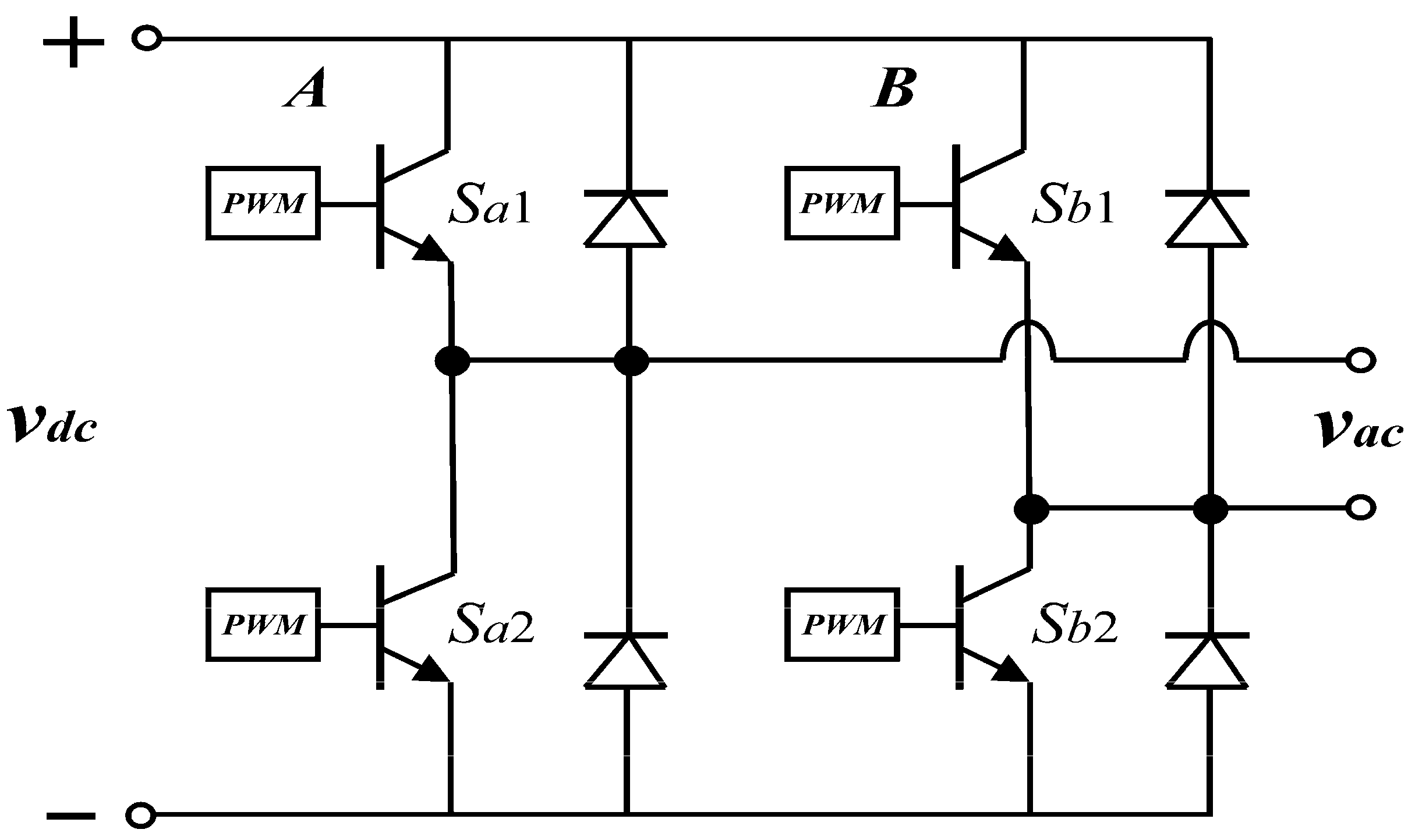
Figure 3 shows a DC/AC converter. The main objective of a DC/AC converter is to generate a sinusoidal AC output voltage, whose magnitude and frequency can both be controlled. It can be observed from
Figure 3 that the DC/AC converter corresponds to a single-phase full-bridge inverter. The switching actions of the inverter are controlled by a PWM scheme with unipolar voltage switching [
28].
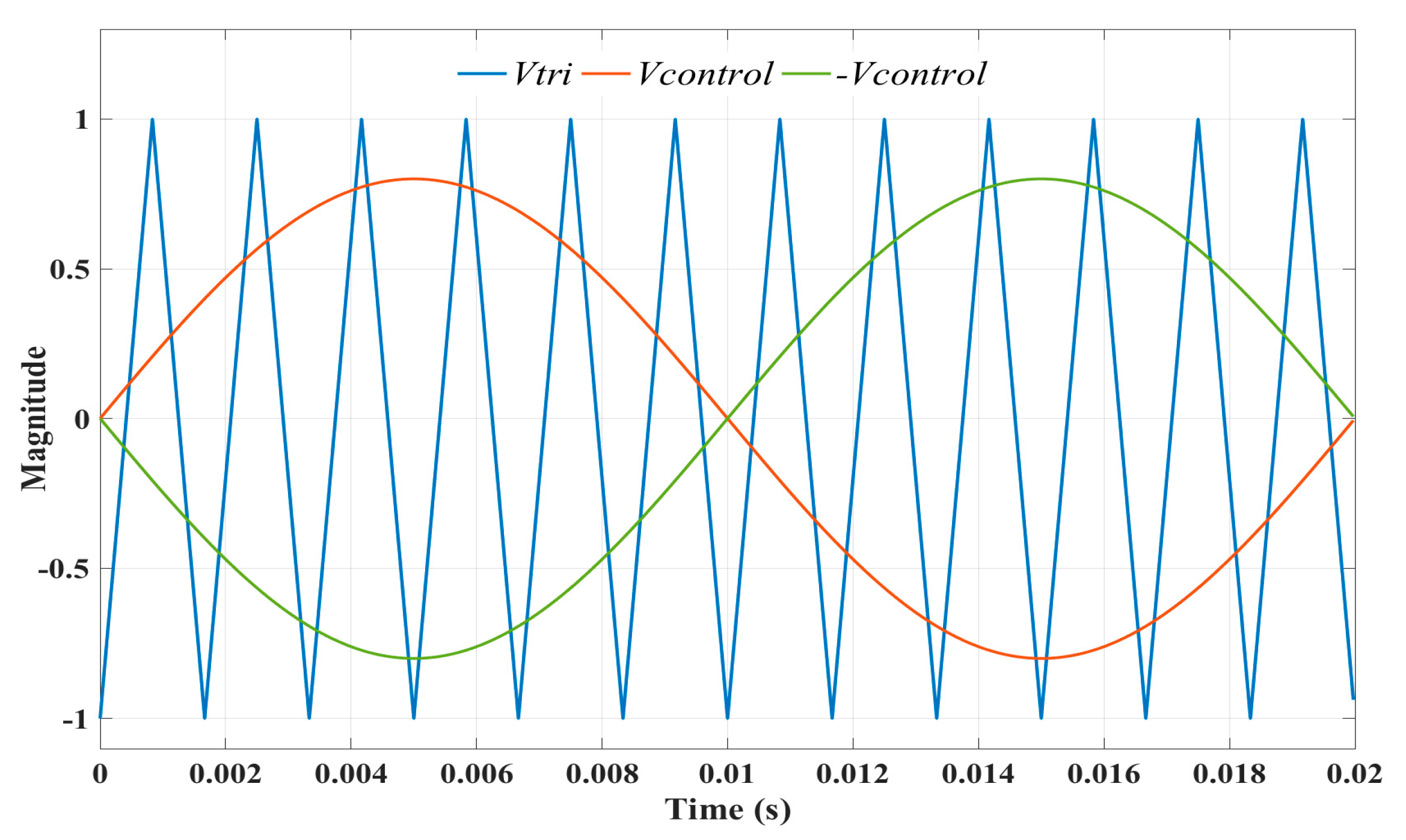
Here, the switches in the legs
A and
B of the full-bridge inverter are controlled separately by comparing the triangular waveform
Vtri (which establishes the switching frequency of the inverter switches) with two sinusoidal signals
Vcontrol and −
Vcontrol (which set the desired fundamental frequency of the inverter output voltage) as shown in
Figure 4, where the peak value of
Vcontrol (the same for −
Vcontrol) is related to
Vtri through the modulation ratio
ma = Vcontrol/Vtri.
It is observed that
ma corresponds also to the ratio between the magnitude of the fundamental component of the output voltage
vac and the magnitude of the input voltage
vdc. The frequency of
Vtri is fixed at several kHz, and determines the order of the harmonics of
vac [
28]. Harmonics in
vac appear as sidebands centered at every two times the frequency modulation ratio
mf =
fs/f0, where
fs is the switching frequency and
f0 is the ac-system frequency.
In the unipolar PWM voltage switching scheme applied to the inverter, the control for leg A is independent of the control of leg B. For leg A, when Vcontrol < Vtri, Sa1 is turned on, otherwise is turned off (Sa2 is always complementary to Sa1). The same rule governs the control of leg B, but using −Vcontrol instead of Vcontrol.
3. Efficient Time-Domain Solution Using the Numerical Differentiation Method
The ND method can be applied to efficiently obtain the periodic steady state of a microgrid with PV energy sources. In principle, a nonlinear power network/component can be mathematically modelled by a set of first-order differential algebraic equations (DAEs), and using some integration routine, such as the TR or Fourth-Order Runge-Kutta (RK4) algorithm [
31], the periodic steady state solution is obtained. This conventional process, known as “brute force” (BF) approach [
9,
32] can be inefficient, as it may require of a considerable time and computer effort. However, TD solution can be significantly accelerated to obtain the periodic steady state solution with the use of Newton type methods [
10,
13]. The mathematical model of DAEs is represented by state space equation:
The extrapolation to the limit cycle of the state vector represented by
x∞ can be calculated as in [
10], i.e.,
where
xi is the state vector at the beginning of the base cycle,
xi+1 is the state vector at the end of the base cycle,
C is the iteration matrix,
is the state transition matrix,
I is the unit matrix,
T is the fundamental frequency period.
The
Φ matrix can be approximated using finite-difference derivative as:
The identification of
Φ is detailed as follows: a base cycle
x(
t) is obtained through the numerical integration of (8) using the BF method during a defined number of cycles, depending of the system damping [
10], and starting from a determined initial condition (e.g., zero condition). Usually, the number of cycles comprises the initial transient. A base cycle can be seen as the last cycle of this initial transient period. Then, the base cycle is sequentially perturbed with a small value at the beginning of the cycle for each state variable. The difference between the base cycle and the perturbed base cycle at the end of the cycle is then evaluated to obtain ∆
xi+1 =
xi+1 −
xi for all the state variables. This allows the sequential identification of the state transition matrix by columns.
With
Φ identified, the iteration matrix
C can be evaluated using (10). Finally, at this point the state vector at the limit cycle can be evaluated using (9). It represents the limit cycle estimation of the state vector. In other words, ND computes
Φ using a column-by-column process. The
kth column of
Φ is
Φk, for
k = 1, 2, …,
n. This column can be computed by perturbing the
kth state, i.e., let
x(
t) →
x(
t) + ∆
xk(
t) and compute
x(
t + T) + ∆
xk(
t + T) by numerical integration of (8) over one period. By letting ∆
xk(
t) to be equal to
ɛU
k, with
ɛ being a small real number, e.g., 10
−6, and U
k the
kth column of a identity matrix of dimension
n, for
k = 1, 2,…,
n, then, by considering (12) we obtain:
and consequently
Each column of Φ can be computed with (15). All n states of the system (8) must be perturbed separately in order to compute the n columns of the sensitivity matrix. Note that n + 1 cycles must be computed to apply (9).
Variants of Solution
Different implementation strategies can be explored for the efficient solution of the microgrid with PV energy sources using the ND method. The identification of the
Φ matrix is the most computationally demanding task during the iterative TD location of the limit cycle. If
Φ and
C are updated at each iteration step using (10) and (11), a Newton process of quadratic convergence to the limit cycle of the state variables results [
10]. On the other hand, it becomes a linearly convergent process if
Φ and
C are kept constant after the first evaluation using (10) and (11). However, this solution process is expected to be significantly faster than the first approach, since a repetitive identification of
Φ is avoided.
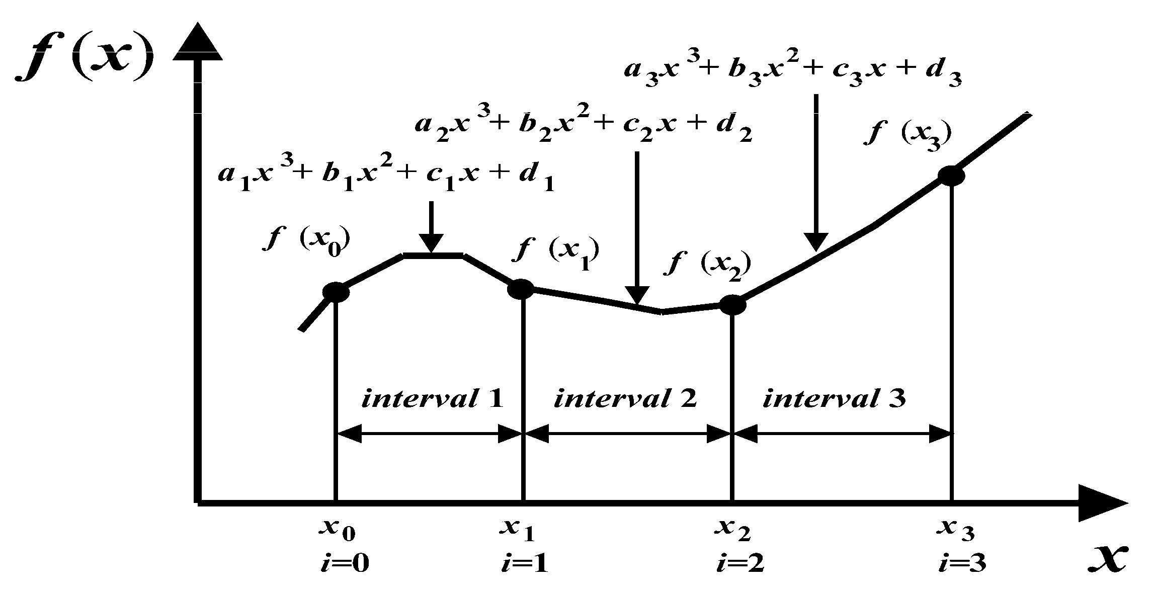
4. Cubic Spline Interpolation
Once the ND method has obtained the steady state solution using the fewest number of data points, it does not represent the final solution and different order harmonics may appear. To avoid this, it is necessary to use an interpolation method to estimate intermediate data points using a mathematical function that minimizes the overall surface curvature, resulting in a surface that passes exactly through the input points. In this work, CSI is used. The objective of the CSI process is to derive a third-order polynomial for each interval of data points [
14]. The polynomial for each interval can be represented by its general form:
Figure 5 helps to explain the notation used to derive cubic splines. The first step in the derivation [
33] is based on the observation that since each pair of knots is connected by a cubic function, the second derivative within each interval is a straight line. Equation (16) can be differentiated twice to verify this observation. On this basis, the second derivatives can be represented by a first-order Lagrange interpolating polynomial as:
where
fi″
(x) is the value of the second derivative at any point
x within the
ith interval. Thus, this equation is a straight line connecting the second derivative at the first knot
f″
(xi−1) with the second derivative at the second knot
f″
(xi).
Next, (17) can be integrated twice to obtain an expression for
fi(x). However, this expression will contain two unknown constants of integration. These constants can be evaluated by invoking the function-equality conditions, i.e.,
f(x) must equal to
f(xi−1) at
xi−1 and
f(x) must equal to
f(xi) at
xi. By carrying out these evaluations, the following equation results:
Clearly, this relationship is a much more complicated expression for the cubic spline for the ith interval than, say, (16). However, please notice that it has only two unknown coefficients, i.e., the second derivatives at the beginning and at the end of the interval f″(xi−1) and f″(xi). Thus, if we can define the proper second derivative at each knot, (18) is a third-order polynomial that can be used to interpolate within the interval.
The second derivatives can be evaluated by invoking the condition that the first derivatives at the knots must be continuous, i.e.,
Equation (18) can be differentiated to give an expression for the first derivative. If this is done for both, the (
i − 1)th and the
ith intervals, and the two results are set equal according to (19), the following relationship results:
If (20) is written for all interior knots, n − 1 simultaneous equations result with n + 1 unknown second derivatives. However, since this is a natural cubic spline, the second derivatives at the end knots are zero and the problem is reduced to n − 1 equations with n − 1 unknowns. In addition, notice that the system of equations will be tridiagonal. Thus, not only we have reduced the number of equations but we have also arranged them in a form that is extremely easy to solve.
6. Test Case
The periodic steady state solution of the single-phase grid-connected PV generation system of
Figure 7 is obtained in the TD framework. The solution is obtained using the BF and ND combined with CSI methods. For the first case, the BF procedure is evaluated with a sampling time-step of 0.1 µs. For the second case, ND obtains the periodic steady state with a sampling time-step of 2.5 µs. Then, the CSI procedure is used just once to reconstruct the waveform. The criterion for convergence of the state variables has been set to 10
−4.
The microgrid has a voltage source, a capacitor bank, five transmission lines, two linear loads, and the PV generation system. The dynamic operation of the system is represented by twelve DAEs. The voltage at the capacitors and the currents in the inductors where chosen as state variables.
Figure 8 shows the equivalent circuit of the single-phase grid-connected PV generation system
The corresponding parameters are contained in
Table 1. The PV array is solved for standard test conditions (STC), i.e., irradiance of 1000 W/m
2 and temperature of 25 °C. The PV system operates at the MPP.
The resultant parameters of the PV array are obtained via the procedure described in
Section 2.1 and presented in
Table 2.
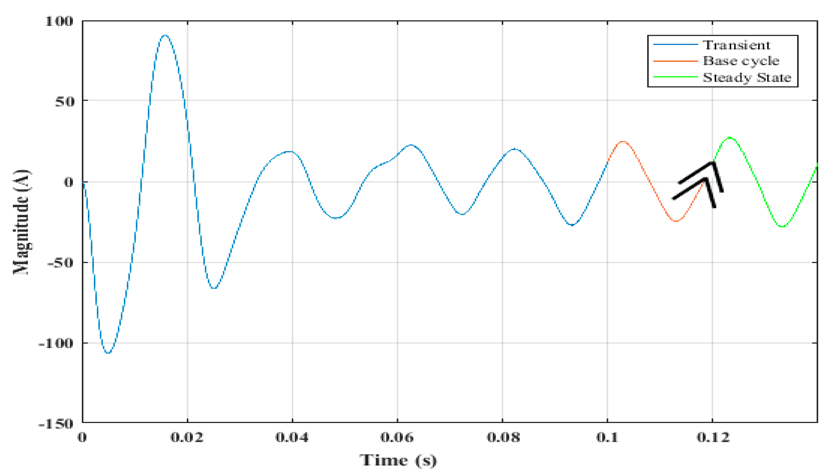
Figure 9 shows the solution to the periodic steady state of the current waveform at PCC using the ND-CSI process. Five initial cycles and a base cycle were obtained before applying the ND method. One cycle of the periodic steady state solution is shown.
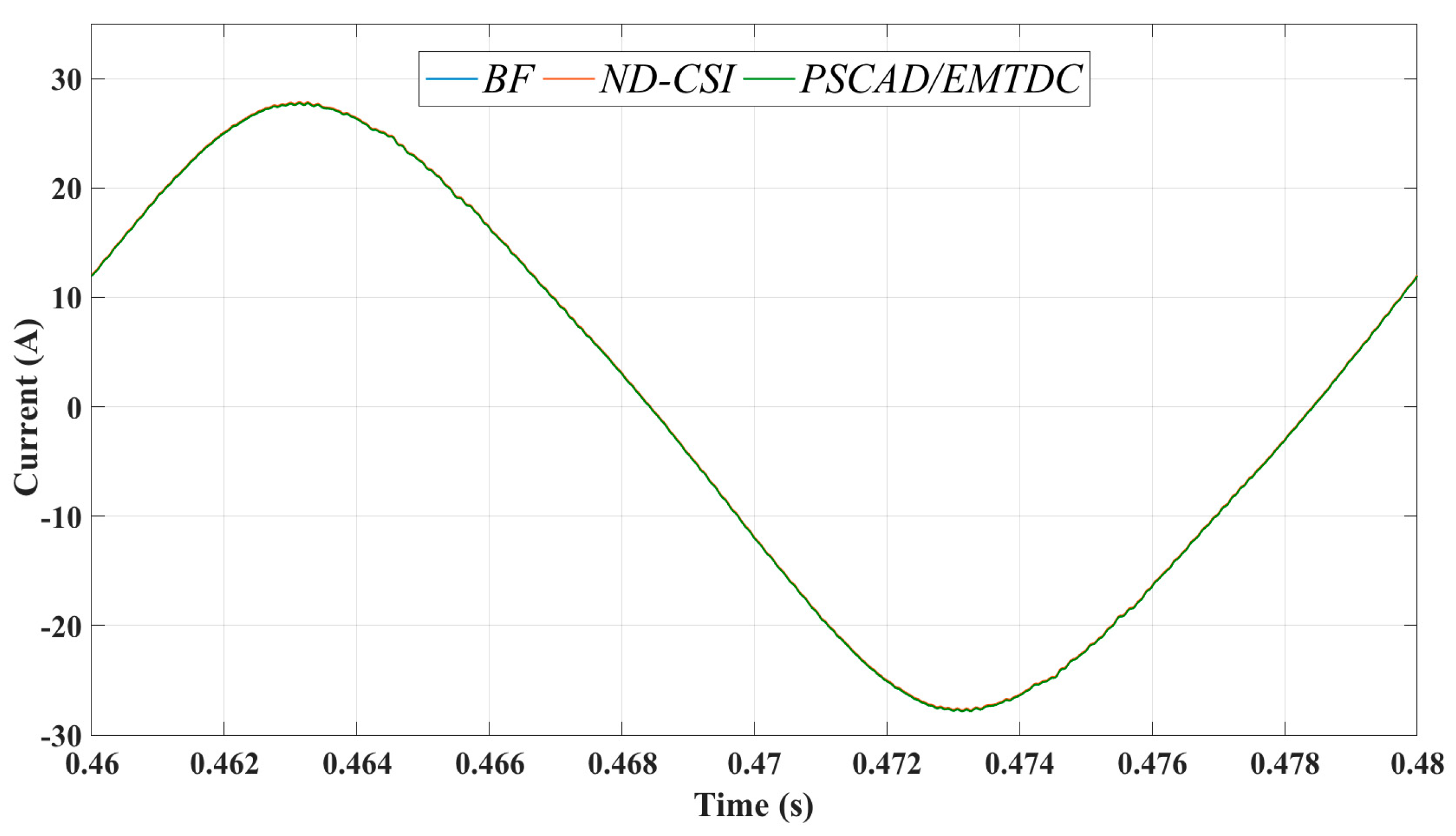
In
Figure 10, the results of the measured current waveform at the PCC obtained with the BF (using TR), ND-CSI, and PSCAD/EMTDC methods, respectively, are illustrated.
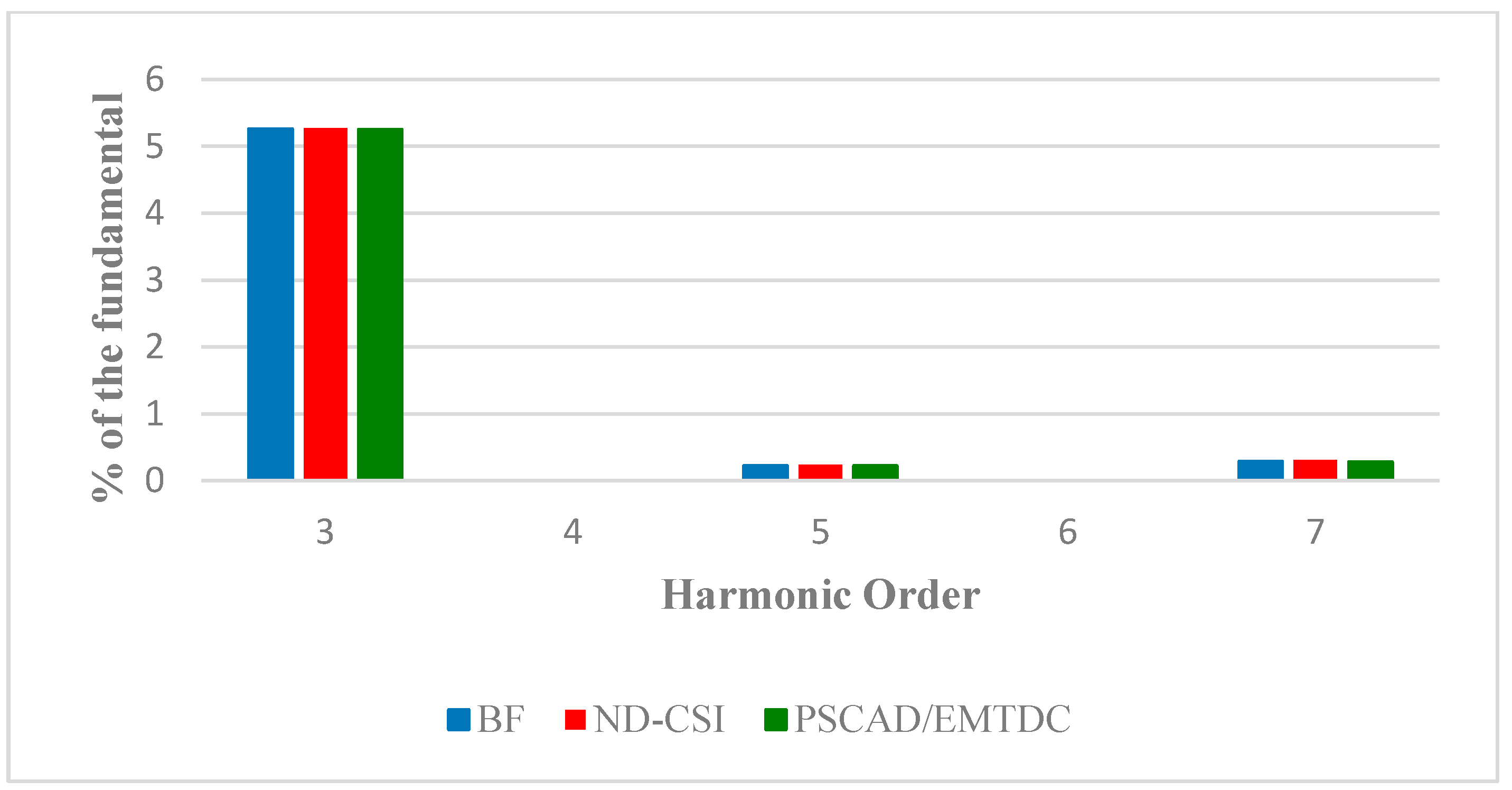
The discrete periodic steady state current waveform is obtained with a reduced time step for the DN method. Then, it is reconstructed using CSI to obtain the final solution with a time step equal to the used by the PSCAD/EMTDC simulator. An excellent agreement between responses can be observed. The corresponding comparison in harmonic content is shown in
Figure 11. The order of the generated harmonics depends on the carrier frequency (
ftri), and of the frequency modulation ratio (
mf). Please notice that the harmonic distortion of the waveform is mainly due to the presence of third, fifth and seventh harmonics. The magnitude of the third harmonic is above the limit allowed by harmonic standards [
34]. Again, a close agreement between the responses obtained with the BF, ND-CSI, and PSCAD/EMTDC are shown.
Table 3 shows the converged values of
d and of the DC components (averages) of voltage and current at the PV array terminals.
Table 3 concludes that the obtained values agree with the MPP as given in
Table 2. Also,
Table 3 reports the THD and powers at the PCC obtained with the BF and ND-CSI methods, respectively. Please observe that the maximum error between responses is negligible, i.e., it is only 0.02% for the
THD in
iPCC.
The algorithm used in this research was implemented with an AMD A8-6410 APU processor with AMD Radeon R5 Graphics, 2 GHz, and 6 GB of DDR3 on-board memory.
Table 4 presents the variants of implementation of the ND method. In terms of the number of full time domain cycles (NFC) required for the convergence to the limit cycle, the BF method took 38 while the ND-CSI with
Φ variable took 18, and ND-CSI with
Φ constant took 30. However, the CPU time needed by the BF method was 348 ms, the ND-CSI with
Φ variable method required 35 ms and the ND-CSI with
Φ constant needed 17 ms. In other words, the ND with
Φ constant is on average two times faster than the ND with
Φ variable. Also, the ND with
Φ constant is 20 times faster than BF method.
Limitations of the Microgrid Modelling
The ND method presents divergence when the microgrid or PV system parameters are erroneously determined.
An initial condition is required to execute the ND method; usually this condition is set to zero. The initial condition can be determined by using different methods, e.g., power flows solution. If the initial condition is not adequately estimated, the ND method may diverge or the time computer effort to converge may be considerable.
PV array parameters can change according to the environmental conditions making difficult to determine a new MPP. Moreover, the microgrid parameters may be recalculated to make the system stable.
The ND method may show difficulties towards convergence when the integration step is too large, i.e., when the number of samples is not sufficient to reconstruct the periodic steady state waveform. Furthermore, the CSI method presents a larger error when rebuilding the signal, taking more computational effort and time.
7. Conclusions
An efficient and accurate time domain methodology to assess the harmonic distortion produced in microgrids with integration of PV sources has been proposed. The TD solution has been substantially enhanced with the combined application of extrapolation to the limit cycle based in the ND method and cubic splines interpolation to the voltage and current waveforms. The computational effort to obtain the time-domain solution has been dramatically reduced when compared against the BF approach, i.e. on average the ND-CSI with Ф variable was 10 times faster than the conventional BF solution and 20 times faster with Ф constant.
It is important to mention that the ND-CSI algorithm with Ф variable needs of a simple modification to become the ND-CSI algorithm with Ф constant. In addition, the ND-CSI approach with Ф constant takes less computational effort than with Ф variable. Therefore, it is worth doing this modification to the method.
The proposed ND-CSI methodology has been successfully verified against the solution obtained with the conventional BF solution and with the PSCAD/EMTDC simulator, respectively. A close agreement between the obtained responses has been achieved. For the reported case study, the maximum error between responses was 0.02%.
At this stage of research, the proposed ND-CSI methodology can be applied for the harmonic distortion assessment of microgrids with integrated photovoltaic sources. Moreover, it can be used for planning, operation and control of microgrids with PV generation sources. Research is under way to incorporate the combined effect of different renewable energy sources. Besides, the execution time of the proposed ND-CSI algorithm can be further reduced by using efficient computational techniques, such as parallel processing based on GPUs. Therefore, this may allow real time applications.


