Data-Driven Predictive Control Applied to Gear Shifting for Heavy-Duty Vehicles

Abstract

In this paper, the data-driven predictive control method is applied to the clutch speed tracking control for the inertial phase of the shift process. While the clutch speed difference changes according to the predetermined trajectory, the purpose of improving the shift quality is achieved. The data-driven predictive control is implemented by combining the subspace identification with the model predictive control. Firstly, the predictive factors are constructed from the input and output data of the shift process via subspace identification, and then the factors are applied to a prediction equation. Secondly, an optimization function is deduced by taking the tracking error and the increments of inputs into accounts. Finally, the optimal solutions are solved through quadratic programming algorithm in Matlab software, and the future inputs of the system are obtained. The control algorithm is applied to the upshift process of an automatic transmission, the simulation results show that the algorithm is in good performance and satisfies the practical requirements.

1. Introduction

Compared with the manual transmission, the automatic hydraulic transmission (AT) not only reduces the intensity of driver’s work, but improves the labor productivity for heavy duty vehicles, especially in characteristics with power shifting ability [1]. The traditional AT is a kind of clutch-to-clutch transmission which the original clutch is separated and the on-coming clutch combined during shifting process. The clutch alternation process should avoid the power interruption, shift overlapping and shocks [2]. The shift process is usually defined as including torque phase and inertia phase. The transmitted torque would change with the oil pressure between the off-going clutch and the on-coming clutch in the torque phase. When the torque transmitted by off-going clutch transfers to the on-coming clutch completely, finally the inertia phase occurs. In this phase, the accurate oil pressure would make the output speed and input speed of transmission synchronous. Based on the experimental data the input speed and output speed changes a little during the torque phase, whereas, it varies intensely in the inertia phase. Therefore, it is crucial to control the clutch speed during the inertial phase for improving shifting quality.

For improving shifting quality several researchers have carried on a large amount of research about the clutch speed tracking control during the inertia phase, and they have already reported successes. As we all known that the mature PID method has been widely used in industry control. Meng et al. [3] used the PID method for improving system characteristics by using a robust 2-D controller defining optimal control parameters, which tracked the desired speed difference trajectory. Mishra and Srinivasan [4] combined adaptive feedback linearization control and sliding mode control to track reference trajectory accurately in inertia phase. The adaptive feedback linear controller calculated the reference oil pressure of the clutch based on the desired clutch speed and real speed, and the collected real pressure and the reference one would be used for input. Gao et al. [5] designed a nonlinear controller with stable input performance using a backstepping method considering system nonlinearity and uncertainty for the inertia phase. Depraetere et al. [6] have designed a two level controller for shifting, the low level of which solved the control variables through building an optimal problem of objective function with constraints, whereas, the high level controller utilized the ILC (Iterative Learning Control) method to update the model and constraints based on the measured data, and the control variables were calculated by the low level controller. Dutta et al. [7,8,9] solved the clutch engagement control problem by using Model Predictive Control, and they emphatically discussed the learning strategy for clutch engagement. Shi et al have developed the way of maintaining the shift quality of automatic transmissions consistent with adaptive control in mass production and with mileage accumulation [10].

In this paper the authors developed model-based learning control (two level nonlinear model predictive control, two level iterative learning control and iterative optimization) and model-free learning control (genetic algorithm and reinforcement learning), and those controllers have been verified by experiments with good control effectiveness.

Most of the mentioned methods for shifting control depend on a detailed model. Since shifting is a complicated and nonlinear process, it is hard to build a theoretical model accurately. The higher order system is also difficult to solve, even when a precise model is obtained [11]. With the rapid development of computer science and technology, a large amount data of during system working had been collected, which includes the system information. When a precise theoretical model is hard to build, data-driven methods could be used to obtain the characteristic information from off-line data and real time date for realizing the optimization control, forecast and evaluation of the system process, which had received a great deal of attention among the control community [12,13,14,15]. In addition, due to some natural advantages, more and more control systems are applied to model predictive control.

In this paper the subspace identification and model predictive control are combined, and a data-driven predictive controller has been designed for gear shifting of ATs. Firstly, the dynamic equation of a planetary gear box was induced by the Lagrange method. Actually, the controller is a kind of model-free control which obtains the system characteristic information to establish the predictive controller from the input and output data by using subspace identification. In the process of clutch speed tracking control, it is necessary to balance the conflicting control requirements. Therefore, the tracking control was changed to a multi-objective optimization problem which is solved by predictive control with considering the constraints in real mechanical system and the improved particle swarm optimization algorithm was utilized for searching optimal solution.

2. Topology Structure of Powertrain System

The powertrain system divided into several subsystems in the simulation model, which includes diesel engine model, torque converter, transmission, drive shaft, longitudinal vehicle model and hydraulic model.

2.1. Diesel Engine Model

By using linear function, sine function and hyperbolic function, the full range of continuous speed regulation characteristic function model was constructed, and it was applied to the engine model shown in Figure 1 [16].

2.2. Torque Converter Model

Based on the pump capacity factor ${\lambda }_p$ and torque ratio $K$, the characteristic curve of the torque converter is determined by the test data which is utilized in the torque converter model [17].

2.3. Transmission Model

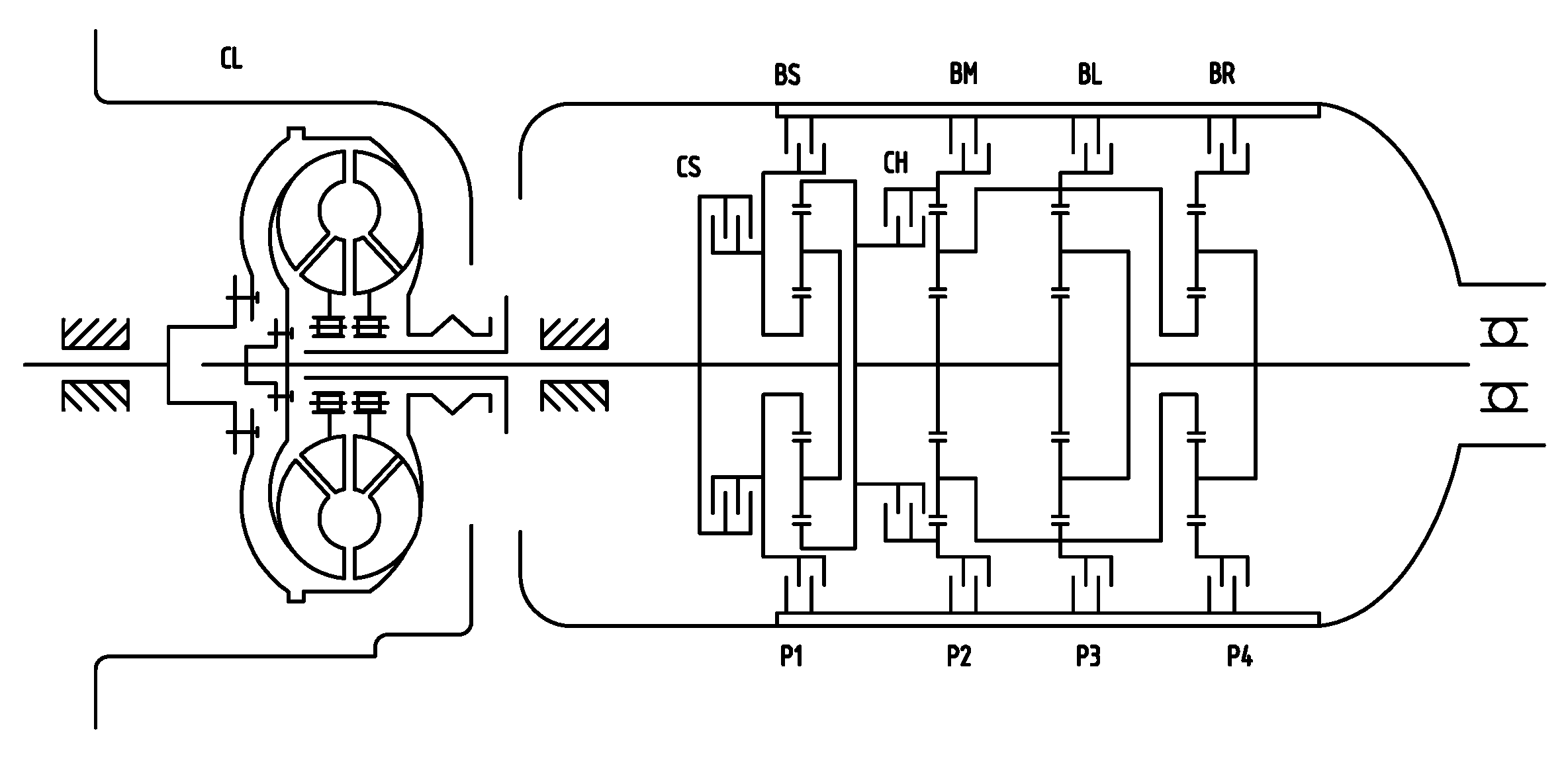
In this study the automatic transmission consists of four planetary systems, two clutches and four brakes. The main work of modelling the AT is focused on definition of the friction model of clutch and the dynamic performances of planetary. For the clutch friction model, the Woods static and dynamic friction model had been used, which is deemed to be a three-state logic function related with the friction torque and reference speed of clutches. Regarding the planetary system, the planetary dynamic equations acquired by the Lagrange method and virtual work principle, which be introduced for modelling particularly in [18,19].

The structure of the automatic transmission was shown in Figure 2, where the torque converter, hydraulic retarder, planetary system, clutches/brakes, hydraulic system and control unit can be seen. The planetary systems represented by P1, P2, P3 and P4. CL, CS and CH indicate the clutches, respectively. In addition, BS, BM, BL and BR represent brakes. When the control unit sends signals to the hydraulic system, the clutches and brakes start working in different ways to acquire the desired ratio. The schedule is shown in

Table 1. Combined clutch/brake schedule.

Gear	CS	BS	CH	BM	BL	BR	Ratio
1	√				√		4.00
2		√			√		2.67
3	√			√			2
4		√		√			1.33
5	√		√				1.00
6		√	√				0.67
R1	√					√	−5.00
R2		√				√	−3.33

, where ‘√’ means engaging.

According to the structure of AT, the Lagrange method was used to establish the dynamic function of the planetary system. Because the fourth planetary didn’t work during shifting from 1st gear to 2nd gear, the reverse gear was neglected during deduction of the function to simplify the modelling. Therefore, the number of planetary systems was reduced to three. The connection type of the planetary set was shown in Figure 3. It can be seen that the ring gear of planetary P1 is connected to the sun gear S2 and sun gear S3, which is named r1s2s3, while the carrier C2 connected ring gear R3 which is named c2r3.

Based on the meshing relationship, the kinematical equation of planetary system was shown as follows:

$$\{\begin{array}{l}{\dot{\beta }}_1{R}_{s1}-{\dot{\gamma }}_1{R}_{p1}={\dot{\alpha }}_1{R}_{s1}\\ {\dot{\beta }}_1(R_{s1}+2R_{p1})+{\dot{\gamma }}_1{R}_{p1}={\dot{\theta }}_1{R}_{r1}\end{array}$$

(1)

$$\{\begin{array}{l}{\dot{\beta }}_2{R}_{s2}-{\dot{\gamma }}_2{R}_{p2}={\dot{\theta }}_1{R}_{s2}\\ {\dot{\beta }}_2(R_{s2}+2R_{p2})+{\dot{\gamma }}_2{R}_{p2}={\dot{\theta }}_2{R}_{r2}\end{array}$$

(2)

$$\{\begin{array}{l}{\dot{\beta }}_3{R}_{s3}-{\dot{\gamma }}_3{R}_{p3}={\dot{\theta }}_1{R}_{s3}\\ {\dot{\beta }}_3(R_{s3}+2R_{p3})+{\dot{\gamma }}_3{R}_{p3}={\dot{\beta }}_2{R}_{r3}\end{array}$$

(3)

where, the terms ${\alpha }_1$, ${\beta }_1$ and ${\gamma }_1$ represent the angular displacement of the sun gear, carrier and pinion in the P1 planetary system, respectively, ${\theta }_1$ represents the angular displacement of the ring gear in P1, sun gear in P2 and sun gear in P3, ${\beta }_2$ represents the angular displacement of the carrier in P2 and ring gear in P3, ${\theta }_2$ represents the angular displacement of carrier in P2, ${\gamma }_2$ represents the angular displacement of pinion in P2, ${\beta }_3$ presents the angular displacement of carrier in P3 and ${\gamma }_3$ represents the angular displacement of the pinion in P3.

For the convenience of operation, ${\dot{\alpha }}_1$, ${\dot{\beta }}_1$ and ${\dot{\beta }}_3$ were selected as the independent coordinate system. After the above six constraint equations are solved, the equation was written in matrix form:

$$\left[\begin{array}{c}{\dot{\theta }}_1\\ {\dot{\beta }}_2\\ {\dot{\theta }}_2\\ {\dot{\gamma }}_1\\ {\dot{\gamma }}_2\\ {\dot{\gamma }}_3\end{array}\right]=A\left[\begin{array}{c}{\dot{\alpha }}_1\\ {\dot{\beta }}_1\\ {\dot{\beta }}_3\end{array}\right]$$

(4)

where $A$ is the coefficient matrix:

$$A=\left[\begin{array}{ccc}-A_1& 1+A_1& 0\\ A_1{A}_2& -(1+A_1)A_2& 1+A_2\\ A_1(A_2+A_2{A}_3+A_3)& -(1+A_1)(A_2+A_2{A}_3+A_3)& (1+A_2)(1+A_3)\\ -A_4& A_4& 0\\ A_1(1+A_2)A_5& -(1+A_1)(1+A_2)A_5& (1+A_2)A_5\\ A_1{A}_6& -(1+A_1)A_6& A_6\end{array}\right]$$

(5)

During the gear shifting, the external force from the hydraulic system is added to the planetary system. The virtual work generated by external torques in virtual displacements is given as follows:

$$\delta W=T_{s1}\delta {\alpha }_1+T_{c1}\delta {\beta }_1+T_{r1s2s3}\delta {\theta }_1+T_{c2r3}\delta {\beta }_2+T_{r2}\delta {\theta }_2+T_{c3}\delta {\beta }_3$$

(6)

It can be seen that the torque would be change when the gear shifts to different gear. Towards the torque of the sun gear in P1, $T_{s1}$, it codetermined by the friction torque $T_{f,CS}$ and $T_{f,BS}$ induced by the clutch CS and brake BS. The torque of carrier in P1, $T_{c1}$, it related with the input torque of the turbine $T_{in}$ and the friction torque from the clutch CS. Due to the fact the carrier in P1 is connected with the sun gears in P2 and P3, the external torque of this component is determined by the friction torque from clutch CH. The carrier in P2 and ring gear in P3 are connected together, and the torque determined by the friction torque of brake BL. The external torque of the ring gear in P2 was codetermined by the friction torque of clutch CS and brake BM. Finally, the torque of carrier in P3 is related with the output torque of transmission, $T_{out}$.

Applying the Lagrange equation to the system, the total energy was taken the derivative with respect to time and calculated by the partial differentiation. The dynamic equation of the AT500 planetary system was acquired about the generalized coordinates, ${\ddot{\alpha }}_1$, ${\ddot{\beta }}_1$ and ${\ddot{\beta }}_3$:

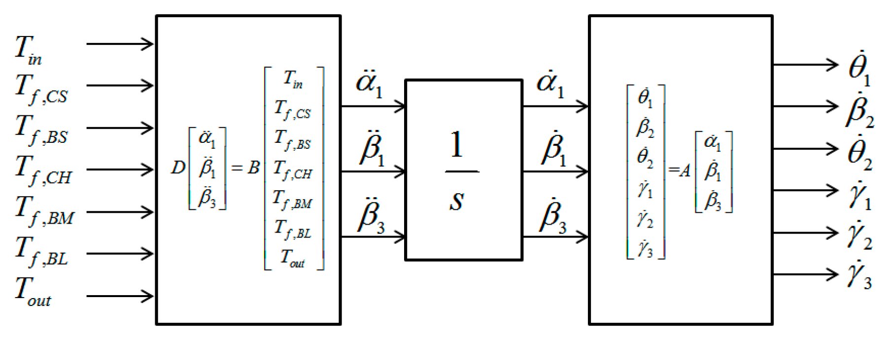
$$D\left[\begin{array}{c}{\ddot{\alpha }}_1\\ {\ddot{\beta }}_1\\ {\ddot{\beta }}_3\end{array}\right]=B\left[\begin{array}{c}{T}_{in}\\ T_{f,CS}\\ T_{f,BS}\\ T_{f,CH}\\ T_{f,BM}\\ T_{f,BL}\\ T_{out}\end{array}\right]$$

(7)

According to Equation (7), the angular speed of the coordinate components was solved when the friction torque of clutches and brakes were known. In addition, the kinematic relationship of all components of AT500 was shown in the following Figure 4.

2.4. Output Shaft and Longitudinal Vehicle Model

For modelling convenience, the longitudinal vehicle model was simplified [20]. The main reducer was considered a simple transmission, and the connection between the reducer and vehicle body was considered as a torsion spring with a certain stiffness which is reduced to a mass block with a certain moment of inertia.

2.5. Control Scheme

For achieving speed synchronization of two relative rotating objects, Meng et al. [1] utilized the piecewise function method to fit the speed difference curve, which the quadratic function was applied in two terminals and the linear function in the middle part. This way insured the difference curve derivative, furthermore, the relative speed variation maintained as zero at the beginning and last moment. Additionally, some research papers have introduced that the cubic function can be used as the curve [21,22,23,24,25]. Over those designations of various difference curves, they aimed to guarantee the relative speed variation as zero and the shifting time fulfilled the requirement since in tracking problems the error between the reference trajectory and real speed is the focus rather than the selection of a reference trajectory. In this paper, the cubic function was used as the reference curve and it expressed as below:

$$\Delta {\omega }^{\ast }(t)=\frac{2\Delta {\omega }_0}{{(t_f-t_0)}^3}{(t-t_0)}^3-\frac{3\Delta {\omega }_0}{{(t_f-t_0)}^2}{(t-t_0)}^2+\Delta {\omega }_0$$

(8)

where, $\Delta {\omega }^{\ast }$ represents the reference trajectory of speed difference, $\Delta {\omega }_0$ represents the speed difference at start moment of inertia phase and $t_0$, $t_f$ represented the start time and end time respectively. We focused on the shifting process from first gear to second gear in this paper which is the alternating process between off-going clutch CS and on-coming clutch BS. When the gear shift starts, the pressure of brake BS is increased gradually. The external torque for AT500 is gradually applied step by step from the clutch CS to the brake BS and it would be split automatically. When the clutch CS is separated totally, it means that the inertia phase starts. Therefore, the target for the pressure control of brake BS is to track the reference trajectory deducing by Equation (8) which is shown in Figure 5.

To optimize the shift quality, the current of electric valve controlled the brake BS $i$ and throttle angle $\theta$ are the control variables, which fulfil $0\le i\le 0.6$ A and $0\le \theta \le 1$. Considering the incremental method utilized in the controller designation, we set the range of control variables satisfying $0\le \frac{di}{dt}\le 3$ A/s and $0\le \frac{d\theta }{dt}\le 4\%$/s, and the increment constraints for the control variables would be calculated according to the step length of simulation and its change rate.

3. Shift Controller Design

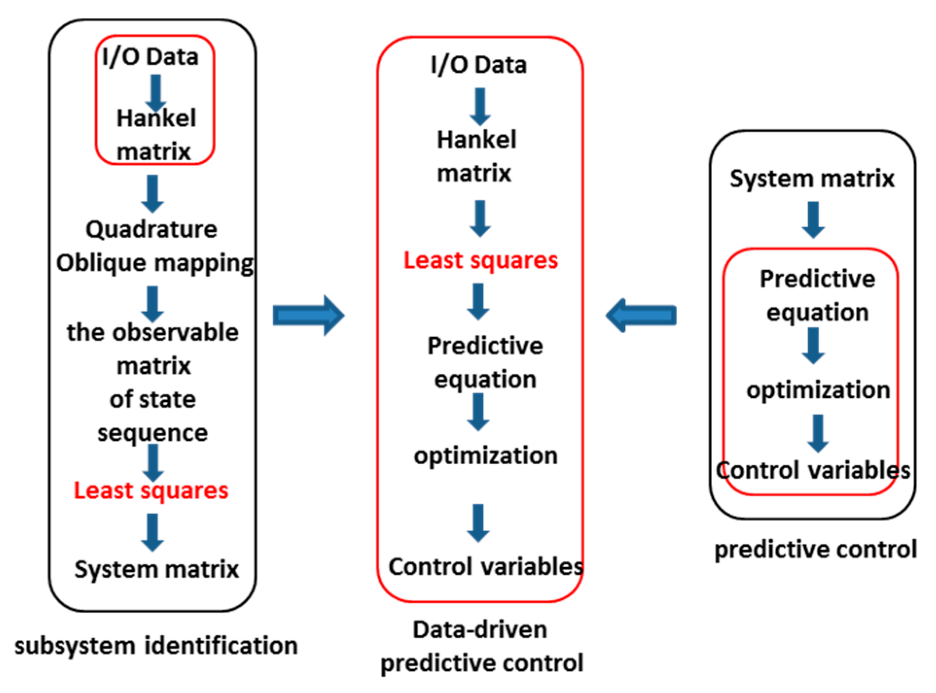
Looking into the mechanism of the system model structure is unnecessary, while the subspace identification just needs a linear algebra tool such as QR without iterative optimization. Therefore, it was easy to achieve and thus has developed rapidly [26]. The main idea is to design an appropriate driving sign for the system, and use it to acquire input and output data. After data normalization, the Hankel matrix built from the input and output data was used to divide it by the QR method and singular value decomposition for estimating the state vectors of the system. Finally, the state space model matrixes A, B, C and D were solved by the least squares method, while the model predictive method was usually used to calculate the future control sequence minimizing the cost function based on the latest measurement at each sampling time in a determined model. Using the first column of those acquired control sequence into the system, the above procedure would be repeated in the next sampling time until the end of the shift. To utilize the data drive predictive method for shifting control, the subspace identification and model predictive control are combined which is presented in the Figure 6.

According the past and future input and output date, the subspace predictors in the prediction equations were acquired by the least squares method [27,28,29,30,31]. The prediction equation was optimized to obtain the future control sequence. Compared with the subspace identification and the model predictive control, it can be seen that the data predictive control is seen as a model-free predictive control method without solving the coefficient matrixes of the state space model, but the predictive equation was acquired by input and output date directly.

The description of data-drive predictive control method is as below:

(1)

Design an appropriate input to acquire the input data u and output data y;

(2)

Formulate the Hankel matrix $U_p$, $U_f$, $Y_p$ and $Y_f$ based on those input and output data;

(3)

Solving the subspace prediction equation for acquiring predictive factor $L_w$ and $L_u$ by least squares method;

(4)

Rewrite the predict equation as the incremental and build the initial relatively speed $\Delta w_p=\left[\begin{array}{c}\Delta y_p\\ \Delta u_p\end{array}\right]$ and reference output sequence $R_e$.

(5)

Building the objective function J and defining the initial constraints;

(6)

Solving the objective function by QP method for acquiring the sequence of the future control variables $\Delta u_f$. The first one would be used into the system input.

(7)

Updating the relatively speed $\Delta w_p=\left[\begin{array}{c}\Delta y_p\\ \Delta u_p\end{array}\right]$ and $R_e$ cbased on the system output.

(8)

Back to the sixth step until the end of shifting.

3.1. Data-Driven Shift Predictor

Considering the optimal control for the inertia phase of shifting, the current of electric valve and throttle angle were regard as the system inputs $u$ and the relatively speed of clutch $\Delta \omega$ was seen as the system output $y$. To stimulate the dynamic characteristics of system, the simulation was carried out in the inertia phase of shifting by using the random input signals.

Usually, the linear time-invariant system is usually described as a state space:

$$\begin{array}{l}{x}_{k+1}=A{x}_k+B{u}_k\\ y_k=C{x}_k+D{u}_k\end{array}$$

(9)

where, $u_k$, $y_k$ and $x_k$ represent the inputs, outputs and state variables, respectively. Assuming known the inputs $u_k$ and outputs $y_k$ at any moment, the Hankel matrix could be defined which was introduced in the thesis [22]. According to the system identification, the output estimate matrix was deduced as follows:

$${\widehat{Y}}_f=L_w{W}_p+L_u{U}_f$$

(10)

The predictive factor $L_w$ and $L_u$ could be acquired by solving the constructed least squares problem. To verify the effect of predictive factors, the first column of the future output matrix calculating by Equation (10) is compared with the test output data based on the simulation model. The simulation results show that the error between the estimated value and test value was very small, and it illustrates that the predictor was useful for estimating the future output date.

3.2. Data-Driven Shift Controller

We substituted the future output sequence into the objective function with considering the constraints. The optimal problem could be deal with as a quadratic programming problem:

$$\begin{array}{l}\underset{\Delta u_f(k)}{\min }\hspace{1em}\frac{1}{2}\Delta u_f{(k)}^{T}H\Delta u_f(k)+G^T\Delta u_f(k)\\ \hspace{1em}s.t.\hspace{1em}C\Delta u_f(k)\le b\end{array}$$

(11)

The increment sequence of future control variables is the solution of the above quadratic programming problem. The first incremental and the control variable of last step are used together to the system, and it will be repeated until the end of shifting.

4. Simulation Results and Discussion

Simulation of controlled object and controller were built by the Matlab/Simulink in this article. Due to the similar process for different gear, we just focus on the shifting from the first gear to the second gear in various working conditions which aimed to verify the effect of controller. In the simulation, the parameters of vehicle and road were changes along with the different conditions, while the parameters of controller maintained as same value.

The main parameters of shifting controller included the number of rows for Hankel matrix $i=50$, the number of columns $j=1100$, the control horizon of the predictor $N_u=4$ and the prediction horizon $N_p=50$. Additionally, the control sequence and incremental constraints were the same as mentioned before. The weight vector, ${\Gamma }_u$ and ${\Gamma }_w$, represented the row vectors after normalization, of which dimensions were 8 and 50, respectively. Because of the high dimensions of weight vector ${\Gamma }_w$, only the weight vector is shown:

$${\Gamma }_u=\left[\begin{array}{cccccccc}0.2789& 0.2789& 0.1317& 0.1317& 0.0609& 0.0609& 0.0285& 0.0285\end{array}\right]$$

(12)

where, ${\Gamma }_u$ reflects the impact on the objective function of different control sequences in future time. It means that the future control sequence was closer to the current time and the cost functions were influenced easier. We assume that the influence of the throttle angle and the current of electric valve were the same in the same moment. In this simulation, we set the start moment of the inertia phase as $t_0=4$ s and it would last about 0.5 s.

Figure 7 reveals that the simulation results in empty condition without slope, where the mass of vehicle $m_v=55,000$, the slope of road $\alpha =0^{°}$, the initial throttle angle $\theta =0.9$, the initial current of electric valve $i=370.2$ and the initial relative speed difference of the brake BS $\Delta {\omega }_0=118.8$.

According to the simulation results, the effect of the designed controller fulfilled the requirements, and the maximum tracking error for angular speed of clutch is about 5.3 rad/s. The throttle angle and the current of electric valve have fluctuations at the beginning of inertia phase that lead to the unsmooth curve of tracking error. Reference [22] has revealed that the turbine speed was affected easily by the control sequence at the beginning of inertia phase. Thereafter, the control sequence and speed difference $\Delta \omega$ start to become smooth. Especially, there is no error between the simulation speed difference and the reference curve at the end of inertia phase. Comparing with the limiting change rate of speed at the beginning and end of inertia phase, the maximum tracking error occurred at the middle part. Due to the requirement only for those two parts, the controller has achieved the desire effect which could be used for shifting.

Since the vehicle works under time-varied conditions, it should be tested under other conditions. The simulation results with empty loss in slope road were shown in the Figure 8, where the mass of vehicle is $m_v=55,000$ kg and the slope of road is $\alpha =5^{°}$. In this condition, the initial electric valve current changed to $i=423.2$ and the initial clutch speed difference is $\Delta {\omega }_0=48.35$ rad/s. It shows clearly that the control variables and output have large fluctuations and takes about 0.06 s to become smooth. In addition, the maximum tracking error is 4.2 rad/s. The results of the full loss in slope are presented in Figure 9, where the mass of vehicle increases to $m_v=72,000$ kg, the slope of road is $\alpha =2^{°}$, the initial throttle angle is $\theta =0.9$, the initial current of electric valve changed to $i=413.5$ and the initial clutch speed difference is $\Delta {\omega }_0=73.84$ rad/s. The simulation results in this condition falls in between the two mentioned conditions where the maximum error is 3.3 rad/s.

5. Conclusions

To reduce the dependency on the detailed model, the subspace identification and model predictive control are combined in this paper. The data-driven predictive control method has been applied to optimize the shifting quality for the inertial phase and it changed the optimization to track reference desired curve. The model-free algorithm utilized the input and output signal data to implement the predictive control by the predictive equation.

When the control variables $\theta$ and $i$ were solved for ensuring the two contradictory indicators that are the shift time and the shift impact, the objective function has been designed considering the constraints for control variables and change rate. The controller was designed in the Matlab/Simulink software, which works out the objective function by the QP with constraints. We used the solved control variables as the input for shifts during the inertial phase, and the simulation results showed that the speed of on-coming clutch tracking the reference curve accurately. Moreover, the simulation result verified the effect of the controller and has robust performance when the mass and road slope change.

In conclusion, the data-driven predictive control not only improves the shift quality but provides a theoretical basis for real-time testing by hardware, which could be utilized in shifting problems for traditional vehicles, hybrid vehicles and electric vehicles without building the transmission model. The results also lay a technical foundation for hardware-in-the-loop tests and real vehicle tests.

References

1. Wang, E.; Tao, G.; Chen, K. A research on power-on downshift control for automatic transmission. Autom. Eng. 2015, 37, 1313–1319. [Google Scholar]
2. Zhao, X.; Yang, J.; Zhang, J.; Zhang, W. Optimizing gear shifting quality with backstepping control for automatic transmission. Trans. Chin. Soc. Agric. Eng. 2016, 32, 27–33. [Google Scholar]
3. Meng, F.; Tao, G.; Zhang, T.; Hu, Y.; Geng, P. Optimal shifting control strategy in inertia phase of an automatic transmission for automotive applications. Mech. Syst. Signal Process. 2015, 60–61, 742–752. [Google Scholar] [CrossRef]
4. Mishra, K.D.; Srinivasan, K. Robust nonlinear control of inertia phase in clutch-to-clutch shifts. In Proceedings of the 4th IFAC Workshop on Engine and Powertrain Control, Simulation, and Modeling E-COSM 2015, Columbus, OH, USA, 23–26 August 2015. [Google Scholar]
5. Gao, B.; Chen, H.; Hu, Y.; Sanada, K. Nonlinear feedforward-feedback control of clutch-to-clutch shift technique. Veh. Syst. Dyn. 2011, 49, 1895–1911. [Google Scholar] [CrossRef]
6. Depraetere, B.; Pinte, G.; Swevers, J. A reference free iterative learning strategy for wet clutch control. In Proceedings of the 2011 American Control Conference, San Francisco, CA, USA, 29 June–1 July 2011. [Google Scholar]
7. Dutta, A.; Ionescu, C.M.; Keyser, R.D.; Wyns, B.; Stoev, J.; Pinte, G.; Symens, W. Robust and two-level (nonlinear) predictive control of switched dynamical systems with unknown references for optimal wet-clutch engagement. J. Syst. Control Eng. 2014, 228, 233–244. [Google Scholar] [CrossRef]
8. Dutta, A.; Depraetere, B.; Ionescu, C.; Pinte, G.; Swevers, J.; Keyser, R.D. Comparison of two-level NMPC and ILC strategies for wet-clutch control. Control Eng. Pract. 2014, 22, 114–124. [Google Scholar] [CrossRef]
9. Dutta, A.; Zhong, Y.; Depraetere, B.; Vaerenbergh, K.V.; Ionescu, C.; Wyns, B.; Pinte, G.; Nowe, A.; Swevers, J.; Keyser, R.D. Model-based and model-free learning strategies for wet clutch control. Mechatronics 2014, 24, 1008–1020. [Google Scholar] [CrossRef] [Green Version]
10. Shi, G.; Dong, P.; Sun, H.Q.; Liu, Y.; Cheng, Y.J.; Xu, X.Y. Adaptive control of the shifting process in automatic transmissions. Int. J. Autom. Technol. 2016, 18, 179–194. [Google Scholar] [CrossRef]
11. Hou, L. Research on Data-Driven Control Scheme Based on Subspace Identification. Master’s Thesis, Northeastern University, Shenyang, China, 2011. [Google Scholar]
12. Hou, Z. On model-free adaptive control: the state of the art and perspective. Control Theory Appl. 2006, 23, 586–592. [Google Scholar]
13. Hou, Z. Highlight and perspective on model free adaptive control. J. Syst. Sci. Math. Sci. 2014, 34, 1182–1191. [Google Scholar]
14. Hou, Z.; Wang, Z. From model-based control to data-driven control: Survey, classification and perspective. Inf. Sci. Int. J. 2013, 235, 3–35. [Google Scholar] [CrossRef]
15. Afram, A.; Janabi-Sharifi, F. Theory and applications of HVAC control systems—A review of model predictive control (MPC). Build. Environ. 2014, 72, 343–355. [Google Scholar] [CrossRef]
16. Zhang, M.; Zhou, Z.; Xu, L.; Li, Y. Continuous mathematic model for governing characteristics of diesel engine. Trans. Chin. Soc. Agric. Eng. 2004, 20, 74–77. [Google Scholar]
17. Yang, C. Dynamic Modeling and Integrated Control for Automatic Transmission Shift Process. Master’s Thesis, Jilin University, Changchun, China, 2014. [Google Scholar]
18. Samanuhut, P. Modeling and Control of Automatic Transmission with Planetary Gears for Shift Quality. Ph.D. Thesis, University of Texas Arlington, Arlington, MA, USA, 2011. [Google Scholar]
19. Meng, F.; Chen, H.; Zhang, T.; Zhu, X. Clutch fill control of an automatic transmission for heavy-duty vehicle applications. Mech. Syst. Signal Process. 2015, 64–65, 16–28. [Google Scholar] [CrossRef]
20. Nezhadali, V.; Eriksson, L. A framework for modeling and optimal control of automatic transmission systems. In Proceedings of the 4th IFAC Workshop on Engine and Powertrain Control, Simulation and Modeling E-COSM 2015, Columbus, OH, USA, 23–26 August 2015. [Google Scholar]
21. Gao, B.; Chen, H.; Sanada, K.; Hu, Y. Design of clutch-slip controller for automatic transmission using backstepping. IEEE/ASME Trans. Mechatron. 2011, 16, 498–508. [Google Scholar] [CrossRef]
22. Lu, X.; Chen, H.; Gao, B.; Zhang, Z.; Jin, W. Data-driven predictive gearshift control for dual-clutch transmissions and FPGA implementation. IEEE Trans. Ind. Electron. 2015, 62, 599–610. [Google Scholar] [CrossRef]
23. Liu, Z.; Gao, J.; Zheng, Q. Robust clutch slip controller design for automatic transmission. J. Automob. Eng. 2011, 225, 989–1005. [Google Scholar] [CrossRef] [Green Version]
24. Depraetere, B.; Pinte, G.; Symens, W.; Swevers, J. A two-level iterative learning control scheme for the engagement of wet clutches. Mechatronics 2011, 21, 501–508. [Google Scholar] [CrossRef]
25. Meng, F.; Tao, G.; Chen, H. Smooth shift control of an automatic transmission for heavy-duty vehicles. Neurocomputing 2015, 59, 197–206. [Google Scholar] [CrossRef]
26. Katayama, T. Subspace Methods for System Identification; Springer: London, UK, 2005. [Google Scholar]
27. Zhou, X. Data-Driven Air Path Predictive Control of Turbocharged Gasoline Engines. Master’s Thesis, Jilin University, Changchun, China, 2016. [Google Scholar]
28. Ma, Y. Research on Predictive Control Based on Subspace in Gas-Collector Pressure of the Coke Oven. Master Thesis, Northeastern University, Shenyang, China, 2013. [Google Scholar]
29. Sun, C. Data-Driven Subspace Methods and its Application in the Prediction. Master Thesis, Northeastern University, Shenyang, China, 2011. [Google Scholar]
30. Li, T. Data-Driven Dual-Clutch Transmission Shift Control. Master Thesis, Jilin University, Changchun, China, 2014. [Google Scholar]
31. Zhang, Z. Data-Driven Predictive Control of Gearshifts and FPGA Implementation for Dual-Clutch Transmissions. Master Thesis, Jilin University, Changchun, China, 2013. [Google Scholar]
Figure 1. Powertrain system.
Energies 11 02139 g001
Figure 2. Diagram of the automatic transmission.
Energies 11 02139 g002
Figure 3. Gear set.
Energies 11 02139 g003
Figure 4. Dynamic characteristic solver of gear set.
Energies 11 02139 g004
Figure 5. The reference trajectory of the clutch speed difference.
Energies 11 02139 g005
Figure 6. Principle of data-driven predictive control algorithm.
Energies 11 02139 g006
Figure 7. Simulation results (vehicle mass m = 55 t ; road slope α = 0 ).
Energies 11 02139 g007
Figure 8. Simulation results (vehicle mass m = 55 t ; road slope α = 5 ° ).
Energies 11 02139 g008
Figure 9. Simulation results (vehicle mass m = 72 t ; road slope α = 2 ° ).
Energies 11 02139 g009