Abstract
The integration of hybrid energy storage systems (HESS) in alternating current (AC) electrified railway systems is attracting widespread interest. However, little attention has been paid to the interaction of optimal size and daily dispatch of HESS within the entire project period. Therefore, a novel bi-level model of railway traction substation energy management (RTSEM) system is developed, which includes a slave level of diurnal HESS dispatch and a master level of HESS sizing. The slave level is formulated as a mixed integer linear programming (MILP) model by coordinating HESS, traction load, regenerative braking energy and renewable energy. As for the master level model, comprehensive cost study within the project period is conducted, with batteries degradation and replacement cost taken into account. Grey wolf optimization technique with embedded CPLEX solver is utilized to solve this RTSEM problem. The proposed model is tested with a real high-speed railway line case in China. The simulation results of several cases with different system elements are presented, and the sensitivity analyses of several parameters are also performed. The obtained results reveal that it shows significant economic-saving potentials with the integration of HESS and renewable energy.
1. Introduction
The dramatic increase of carbon emissions is driving global climate change and poses risks for human and natural systems [1,2], and a worldwide consensus on reducing atmospheric greenhouse gases (GHGS) has been reached [3,4]. As for China, the government committed a reduction of carbon emission intensity by 18% during the 13th Five-Year Plan period (2015–2020) [5]. A joint report from the International Energy Agency (IEA) and the International Union of Railways (UIC) shows that the transport sector accounted for 24.7% of global carbon emissions and the rail sector accounted for 4.2% of total transport carbon emission in 2015, while the corresponding proportion in China is 10.6% and 15.3% [6]. Most noteworthily, the railway-related energy consumption and carbon emissions per passenger-km increased by 44.1% and 96.8% between 2005 and 2015 in China respectively, largely as a result of the rapid expansion of the high-speed railway (HSR) network [6]. Consequently, energy savings in railway systems and in HSR systems have received considerable critical attention.
A few approaches provide insights for energy saving, such as the use of regenerative braking energy and renewable energy techniques. Due to the high speed and colossal traction power of high-speed trains (HSTs) with pulse width modulation-based four-quadrant converters [7], considerable regenerative braking power (RBP) is produced in their braking mode. For instance, the maximum braking power of a CRH-380AL electric multiple unit (manufactured by China Railway Rolling Stock Corporation, Qingdao, China) can be up to 20 MW. Therefore, there is a growing application of energy storage systems (ESSs) in railway systems to store this massive braking energy [8]. Currently, industrial applications of onboard ESS for braking energy recovery include the Sitras SES of Siemens, the MITRAC energy saver of Bombardier and the STEEM project of Alstom [9,10,11]. However, the limitations of size and weight have presented an obstacle to the application of onboard ESSs in HSRs. By comparison, wayside ESSs can be a better solution. Moreover, the intersections of railway networks and renewable energy sources (RES) are propitious to the utilization of local renewable energy. For instance, the Lanzhou-Xinjiang HSR line crosses the north-western regions of China with rich solar and wind energy, while there is no access to local RES consumption. With regard to the way that RBP and RES are used, aside from supplying to the HSTs, they can also be utilized to charge the energy storage devices, e.g., HESS, for further usage. Therefore, increasing the utilization rate of RBP and RES via HESS helps achieve the energy saving goals.
Moreover, cost savings for rail operators can also be implemented from another point of view. In the current railway power systems, the dramatic stochastic volatility of traction loads and the harsh requirements for overload capacity of traction transformers result in the extremely low utilization rate of traction transformers and high demand charge. Besides, the RBP fed back to the grid contains a large number of harmonic components and negative sequence components because of the single-phase asymmetry of traction loads, seriously jeopardizing the safety and stabilization of the utility power system [12]. Consequently, a resulting penalty bill is charged. To this end, there is great potential for cost saving through the application of HESS and management of energy flows.
Smart grid technologies present the potential of energy management in railway power supply systems. The battery sizing and energy management in smart grids have been extensively studied in recent years, such as grid-tied photovoltaic (PV) systems [13,14], wind farms [15], active distribution systems [16] and microgrids in stand-alone mode or grid-connected mode [17,18,19,20,21,22]. However, the characteristic of traction loads differ significantly from conventional loads. Therefore, the sizing and dispatch strategy of HESS need to be re-examined when applied to electrified railway systems.
Numerous researchers have focused on solving the above problems in the railway systems. Khayyam et al. [23] developed a railway energy management system (REM-S) architecture by coordinating loads, regeneration, storage, and distributed energy resources for optimal energy use. It offers the inspiration of applying the research achievements of smart grids to railway systems. Generic hybrid railway power substation (HRPS) architectures for DC and AC systems were proposed in [24] by integrating RES and storage units with railway systems. Based on the HRPS system in [24], corresponding fuzzy logic energy management strategies were developed in [25,26] for feasibility analysis. However, the battery degradation and replacement were ignored. A hierarchical structure, including on-route trains energy consumption optimization and traction substation energy flows management, was identified in [27,28] to minimize the electricity bill. However, no capital cost of storage devices was considered. In [29] a smart railway station energy management system model was formulated for the utilization of braking energy, and the initial state of charge (SOC) was highlighted in particular as the uncertain factor. Unfortunately, it merely concentrated on the reduction of electricity bill of power consumption and paid little attention to the comprehensive cost analysis. In [30] an optimization model of battery energy storage system (BESS) operation strategy was developed for the maximization of owner’s net benefit. However, the evaluation of degradation cost was off-line, i.e., it was not included in the optimization model. Furthermore, regenerative braking energy of metro trains was not considered. In [31] the author proposed a methodology for optimal dispatch of railway ESS with RES and braking energy, while the investment cost was not taken into consideration. In [32] the optimal sizing of HESS for braking energy utilization was studied, yet the battery lifetime was estimated simply based on the cycles, and the depth of discharge (DOD) of each cycle was ignored, thus the estimation of battery lifetime and daily cost need to be further improved.
The aforementioned studies and many other studies not referred here give approaches to sizing of energy storage devices or energy management in railway systems from different perspectives, while the comprehensive cost study within the time scope of project period is ignored, and a more accurate on-line methods for battery lifetime estimation are not considered. Accordingly, this paper aims at addressing this problem. The highlights of this paper can be outlined as follows:
- The interaction of HESS sizing and daily scheduling of HESS within the time scope of project service period considering battery degradation are formulated via a bi-level model.
- The electricity bill for rail operators is largely reduced through peak shaving of traction loads, utilization of braking power and the mitigation of bill penalties for power fed back to the utility grid.
- The impact of different electricity pricing schemes, length of project service period and initial SOC of HESS are also analyzed.
The rest of this paper is structured as follows: Section 2 introduces the general architecture of RTSEM system and descriptions of all the elements included. Section 3 and Section 4 present the problem formulations of the master level and slave level respectively. In Section 5, a grey wolf optimization approach with CPLEX solver embedded is proposed. In Section 6 the case study is performed and relevant results are given. Finally the conclusions are reached in Section 7.
2. System Description
2.1. Block Diagram of the System and Model
In conventional electrified railway systems, the 25 kV traction network supplies single-phase AC at the power frequency for HSTs. As the phases of adjacent power supply sections are different, all sections must be kept strictly isolated to prevent the risk of mixing out-of-phase supplies, which is achieved by neutral sections. In this study, a scheme of RTSEM system is illustrated in Figure 1, which is based on the architecture of hybrid railway power substation proposed in previous studies [24,27]. The power direction and corresponding symbol convention are presented as well. The RTSEM system is mainly composed of utility grid, PV generator, battery storage system, ultracapacitor (UC) storage system and HSTs. It is important to highlight that HSTs have dual properties of “load” and “power source”, depending on whether the train is in traction mode or regenerative braking mode. This special feature of HSTs differs from conventional power load greatly, increasing the diversity of operation mode and the complexity of energy management though, yet nevertheless showing quite economic-saving potentials.
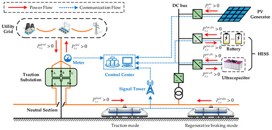
Figure 1.
Structure diagram of the RTSEM system.
Note that a study of the entire HSR line containing plenty of traction substations (TSSs) and power supply sections may lead to a large-scale problem. As different power supply sections of an HSR line are electrically disconnected via neutral sections, this paper concentrates on each power supply section individually.
Figure 2 illustrates the block diagram of the bi-level model proposed in this paper. The upper blocks of computer simulation and scenarios are the pretreatment process, which offers input parameters for the following model. In this study, the sizing of HESS and comprehensive cost calculation are implemented within the time scope of the project service period. A bi-level model is thus proposed in order to reflect the close association between the total project cost and diurnal scheduling of HESS. The master level model concentrates on the optimal sizing of HESS and the slave level model involves the diurnal scheduling of HESS. As the decision variables of master level model, the power rating and capacity of battery and UC are regarded as the boundary parameters of slave level model. Battery lifetime, HESS operation hours and daily electricity cost calculated in the slave level model are returned to the master level model for the assessment of certain types of cost accordingly. The diurnal operation of HESS is regarded as repeated within the project service period.
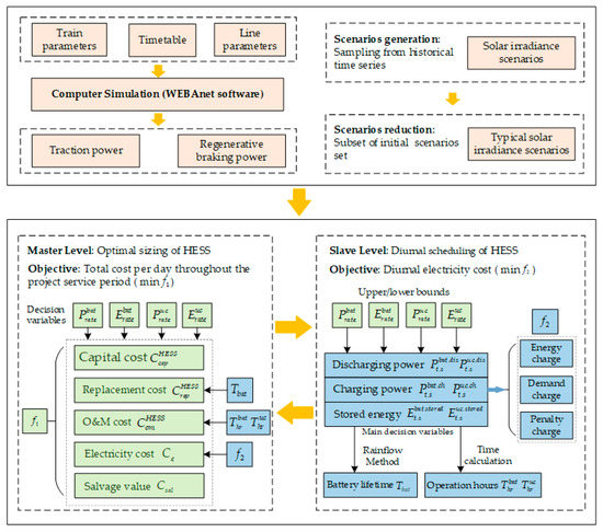
Figure 2.
Overview of proposed bi-level model optimization.
2.2. Traction Load and Regenerative Braking Power
As the input parameters of the proposed model, railway traction load and RBP profile should be determined in an accurate and efficient way. Two common methods for traction load prediction include [31]:
- Computer simulation method based on traction and power supply calculation.
- Statistical model or sampling method based on measurement data from the meter installed in the traction substation.
For ease of the analysis of different operation conditions, the computer simulation method is adopted here. A lot of parameters of HSTs and HSR lines are required in advance in the computer simulation method, e.g., the traction force, running resistance and braking force of HSTs, slope, curve radius and speed limitation of HSR lines, and the equivalent impedance and admittance of traction power systems [31]. Normally, these required parameters can be obtained from the railway investigation and design institutes. Benefitting from the great advances of simulation software for the load processes of traction power supply systems, forecasting of railway traction loads and regenerative braking power can be easily implemented based on the aforementioned parameters and timetables preset by railway operators. In this study the traction simulation is performed via the commercial software ELBAS WEBAnet v3.121 (SIGNON Group, Berlin, Germany) [33].
On account of the computational resource limitations and for saving computation time, sampling and processing of the simulation results should be designed appropriately. The sampling time interval in [29] is determined as 1 min considering the short braking time. A time period reduction method is applied in [31,32] via combining short 30 s time periods to form longer time periods, yet with the defect of unequal duration between different time periods. The sampling time of power profile and the scheduling time interval of HESS are determined as 1 min in this study, based on the fact that power profiles of traction load and HESS do not change much during this short period.
2.3. Uncertainty Representation of PV Generation
When we focus on the sizing configuration and long-term planning of HESS within the time scope of project period, the stochastic characteristics of weather conditions have to be included. Typically, a series of scenarios and corresponding probabilities are used to describe the stochastic process and data process [34], thus the scenario-based technique is adopted in this section.
Renewable energy represented by PV generation is taken into account in this paper for the nearby consumption of renewable energy. With regard to the scenarios generation, in order to describe the uncertainty of PV generation as far as possible, the annual solar irradiance profile is used here to generate 365 different scenarios.
Significant computational resources and time cost are required when all the scenarios are included in the stochastic bi-level model, thus a tradeoff between the solution accuracy and computation speed should be achieved [35,36,37]. Aiming at dealing with the contradiction of computational complexity and time limitation, scenario reduction method is developed in previous studies [34,38,39]. In [34] the scenario reduction algorithms reject the low-probability scenarios and aggregate those that approximate to each other in light of probability metric, forming a scenario subset that represents a relatively good approximation to the initial scenario set in terms of statistic metric:
Various algorithms can be applied for scenario reduction, including the fast backward method, fast backward/forward method and fast backward/backward method [34,38]. In view of the different computation performance and accuracy between these algorithms, they are applicable for different occasions, such as the problem size and target precision [35,40,41]. For example, the forward method provides the best solution accuracy with the largest computational resource consumption, while the fast backward method requires the least computational effort at the cost of lower accuracy [35,41]. Therefore the forward method is utilized to generate four representative scenarios for scenario reduction in this study, as shown in Equation (1), considering a small number of scenarios need to be reduced.
2.4. Hybrid Energy Storage Systems
Energy storage systems play a key role in the cost-saving benefits of RTSEM by means of discharging during peak traction load periods and charging during regenerative braking periods. Two types of widely applied energy storage systems include the high energy density type, represented by batteries, and high power density type represented by UC. Batteries have good performance in terms of high energy density and mature manufacturing process, whereas lifetime cycles and power density are limited [42]. By contrast, UC have advantages of high power density, fast response, lower maintenance cost and extremely long cycle life [8], while low energy density and quite high energy capacity cost are the main obstacles to the spread application of UC. HESS is proposed with the intention of combining the batteries and UC to obtain both high energy and power density, and thus has an obvious advantage over the single type of energy storage system, especially for the application of peak load shaving and regenerative braking power absorbing in the high-speed railway system. In general, the UC’s advantage of long cycle life and fast response make it suitable to capture the railway power peaks and valleys in high frequency, while batteries are more suited for low frequency operation [31,32]. Accordingly, HESS is adopted in this study for the better energy saving performance.
3. Master Level: HESS Sizing Problem Formulation
3.1. Battery Degradation Analysis
When applied into the electrified railway systems, HESSs are operated to coordinate with the traction loads, a kind of shock load with dramatic stochastic volatility. It is assumed that UC can serve for the entire project period and the batteries degradation analysis is considered, as a result of the fact that the lifetime of UC is less affected by the cycles, while batteries are more likely to suffer from the frequent fluctuations and plenty of cycles of traction load in view of the limited life cycles [42].
As the key connection between the master and slave level model, battery lifetime indicates the fact that the diurnal operation strategies of HESS have a great impact on the replacement cost, thus an optimal balance should be achieved between the performance of HESS and the replacement cost, and that is the problem this paper tries to solve.
The disadvantage of limited lifetime cycles results in a more severe aging of batteries during the operation of HESSs, thus an appropriate method should be utilized to evaluate the aging rate of batteries within the considered time scope. There are lots of approaches for batteries lifetime estimation, in which the number of battery cycles calculation method is utilized in this study. Generally, battery cycles can be divided into two types, including full cycles and partial cycles [43]. A full cycle is defined as a combination of a charge half cycle and a discharge half cycle with equal starting SOC and ending SOC. Accordingly, a partial cycle is defined as a charge or discharge progress with unequal starting SOC and ending SOC. By means of the rainflow counting method, full cycles and half cycles can be extracted from a series of charge or discharge sequences. For further knowledge of counting methods readers may refer to [44].
The flow chart of the rainflow counting method is presented in Figure 3. The functions of this method include the extraction of two types of cycles and the determination of corresponding DOD of each cycle. According to manufacturer’s data, number of battery cycles to failure as a function of depth of discharge D is presented in Equation (2), by applying interpolation with least square method. The coefficient α1, α2, α3 and α4 are 24,090, −9.346, 6085 and −1.319 respectively in this study according to [45]:
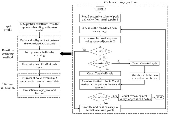
Figure 3.
Flow chart of batteries lifetime estimation.
Each cycle corresponds to an aging rate. In order to establish the association between the lifetime and aging rate of each cycle, accumulated aging rate AR is derived in Equation (3) by adding up the total aging rate based on the total cycles () of batteries within a day, where is the aging rate for each cycle i. Coefficient αi is 1 when cycle i is a full cycle and 0.5 when cycle i is a half cycle, since it is regarded that the effect of a half cycle is the half of a full cycle. Therefore the expression of lifetime in years can be derived in Equation (4):
Note that according to [45], an adverse effect is on the lifetime once the operating temperature is over 20 °C. A constant operating temperature of 20 °C is assumed in this study for the sake of simplicity and the related cost is included in the Balance of Plant (BOP) cost that is introduced in Section 3.2.1.
Figure 4 shows the identification of full cycles and half cycles from the input signal via the process of the rainflow counting method.
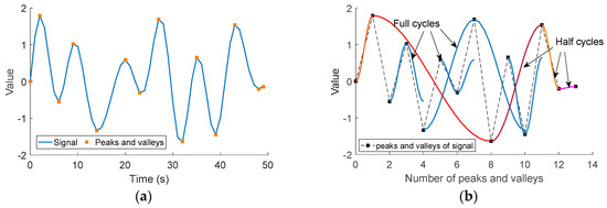
Figure 4.
Demonstration of the rainflow counting algorithm: (a) Extraction of peaks and valleys from the input signal; (b) Identification of full cycles and half cycles.
3.2. Objective Function of the Master Level Model
In the following Equation (5)
where and are the rated power and total capacity of battery; and are the rated power and total capacity of UC. Note that the investment cost of PV is not considered within the scope of this paper. Each cost in this study is expressed as the daily cost.
3.2.1. Capital Cost
The HESS is mainly composed of battery banks, UC banks, power conversion systems (PCS), and other devices related to BOP [46,47], such as protective devices, monitoring and control systems and so on. The PCS cost is associated with the designed power level of PCS, which is considered as the power rating of battery and UC respectively in this paper. BOP cost is typically related to the rated power, thus the diurnal capital cost of HESS can be expressed as:
where is the operation days of HESS within a year (365 in this paper); (CNY/MW), (CNY/MWh) are the specific cost of per unit of power rating and capacity of battery respectively; (CNY/MW), (CNY/MWh) are the specific cost of per unit of power rating and capacity of UC respectively; (CNY/MW) refers to the unit cost associated with BOP; CRF denotes capital recovery factor, which is the ratio of a constant annuity to the present value of receiving that annuity for a given length of time [16,48]. is the project service period in years and is the annual discount rate. The definition of capital recovery factor can be described using Equation (7).
3.2.2. Replacement Cost
As the master level concentrates on the long-term planning and the lifetime of battery is normally far less than the project service period due to the limitation of total number of cycles until end-of-life, thus battery needs to be replaced every specific period. From this point of view, diurnal operation strategies of battery not only affect the performance of traction load peak shaving and penalty bill avoidance in the short term, but also impact the life cycle cost and replacement of battery in the long run. It is assumed that UC and devices related to BOP can serve all through the project period and no replacement is taken into consideration, considering its extremely long cycle life. The total replacement cost per day is expressed in Equation (8):
where (CNY/MWh) is the replacement cost of the capacity of battery. denotes the battery lifetime, of which the calculation method is introduced in Equation (4); PVF denotes the present value factor which is used to derive the present value of a receipt of cash in the future. Present value factor is defined as Equation (9); is the total times of battery replacement during the project period and k represents the index of replacement. is defined in Equation (10):
where represents the rounding up operand.
3.2.3. Operation and Maintenance (O&M) Cost
The diurnal O&M cost is divided into fixed O&M cost and variable O&M cost in [47], it can be expressed as:
where and are fixed O&M cost per unit of power rating associated with battery and UC, in CNY/MW; and are variable O&M cost per unit of power rating associated with battery and UC, in CNY/MW; and represent the operation time of battery and UC during a day, in hours, which can be obtained from the Equations (44) and (45) in the slave model of diurnal HESS scheduling.
3.2.4. Salvage Value
Salvage value is the estimated resale value of an asset at the end of its useful life. In the final year of the project service period, the salvage value of the system primarily depends on the recovery value of batteries that have not reached the failure of their lifetime:
where is the depreciation coefficient for the recovery of battery storage banks. SFF denotes the sinking fund factor which is used to calculate the future value of a series of equal annual cash flows. The definition of sinking fund factor can be presented as follows:
3.3. Constraints of the Master Level
The sizing of the HESS involves finding the optimal power rating and energy capacities of batteries and UCs aiming at minimizing the total cost within the time horizon of project service period. Equations (16)–(19) state that these decision variables are limited by upper and lower bounds, which can be determined according to the types of ESS and the traction load of traction substations. Besides, Equations (2)–(4) performing the battery lifetime estimation are also a part of the constraints in the master level model:
4. Slave Level: Diurnal Dispatch Problem Formulation
Under the restrictions of power capacity and energy capacity of HESS and power balance among the RTSEM system, slave model focuses on the optimal scheduling of HESS during a day, aiming to minimize the electricity cost via traction load peak shaving and avoiding penalty bill for the railway operators.
4.1. Objective Function of the Slave Level Model
As a major role of commercial and industrial (C&I) electricity consumer, electrified railway operators are primarily charged based on two aspects in China: energy consumption and demand, i.e., with a two-part tariff [49]. In addition, other regulations and tariff rules imposed by the State Grid Corporation of China should be considered. The composition of electricity charge can be expressed as follows:
- Energy consumption charge. Electric utilities installed in the traction substation meter the energy consumption supplied by utility grid, and this charge is obtained through the energy consumption and corresponding energy price.
- Capacity charge or demand charge. This part of charge is associated with the construction cost of power plant, transmission lines and other facilities. Typically two options are offered to the C&I consumers: transformer-capacity-based charge or peak-demand-based charge. The former is related to the capacity of transformers, and the latter depends on the maximum value of the averaged active power consumption in successive 15 min time intervals, during a billing month (or a day in this study, as the diurnal operation of the elements in RTSEM system is regarded as repeated within the project service period). The latter option is applied in this paper.
- Penalty charge. HSTs have been widely put into service in HSR lines in China. Part of the RBP is absorbed by HSTs running in the same power supply section, and the rest returns to utility power system. However, the RBP fed back to the grid contains a large number of harmonic components and negative sequence components, bring potential threats to the utility power system. Therefore, a bill penalty is charged for the traction power fed back to the utility grid.
According to aforementioned tariff rules, objective function of slave model is the diurnal electricity bill for railway operators, including energy consumption charge (ECC), demand charge (DC) and penalty charge (PC). They are calculated as follows:
- The energy consumption charge can be expressed as:
- The demand charge is derived as:
- The penalty charge is as follows:where is the probability of PV generation scenario; (MW), (CNY/MW) are active power supplied by the utility grid and corresponding electricity price signal; (MW) and (CNY/MW) represent the regenerative braking power fed back to utility grid and the penalty charge; (CNY/MW) denotes the electricity price of peak demand power; is the discretization time interval; is the average active power consumption during each 15-min interval and T refers to the total number of time intervals during a day.
Due to the nonlinearity of the maximum function in Equation (22), linearization is applied in Equations (25) and (26) in order to formulate the diurnal scheduling problem as a mixed-integer linear programming (MILP) model.
where is an additional time-independent variable representing the peak demand power during a day.
4.2. Constraints of the Slave Level Model
4.2.1. Power Balance
All participants in the RTSEM system are constrained by the active power balance, which is presented in Equation (27). It states that the active power supplied by the utility grid (), PV generator (), battery (), UC () and regenerative braking power () must meet the requirement of railway traction load (), battery charging (), UC charging (), or even feed superfluous power back to grid (), inevitably resulting in penalty charge of course.
4.2.2. HESS Constraints
The charging or discharging power and stored energy of the HESS are constrained by the physical characteristics of battery and UC at any time interval. All the inequality and equality constraints related to the operation of HESS in this proposed diurnal dispatch problem are organized as follows. Equations (28) and (29) imply the relationship between discharging or charging power and remaining energy at adjacent time intervals with efficiency and self-discharging rate taken into account. Generally a limitation of state of charge is set so as to avoid over-discharge and extend the lifetime of battery [50,51,52], so Equations (30) and (31) indicate that the stored energy in battery and UC must be bounded by a predefined upper and lower bounds according to the actual parameters of selected type of storage systems. Equations (32)–(35) set up the limitation of discharging and charging power, which means that both the power rating and available energy variation at time interval can decide the upper bound of power. Equations (36) and (37) state that stored energy at initial stage equals that at final stage for the convenience of scheduling in the next day, as the diurnal operation of HESS is regarded as repeated within the project service period. Equations (38)–(43) demonstrate the fact that charging status cannot coexist with discharging status simultaneously. Equations (44) and (45) are applied to calculate the operation hours of batteries and UCs during a day.
where and are the self-discharging rate of battery and UC; , , and are discharging and charging efficiency of battery and UC; is duration of time interval in hours (1 min in this paper); , and denote the minimum, maximum and initial state of charge of battery respectively; , and represent the minimum, maximum and daily initial state of charge of UC respectively; binary variable and are 1 if battery or UC is in discharging state, and 0 otherwise; binary variable and are 1 if battery or UC are in charging state, and 0 otherwise; binary variable and equal 1 if battery or UC are in operation mode (charging or discharging) and 0 otherwise.
It is noted that the rated power and capacity of battery, and the rated power and capacity of UC in this HESS constraints of slave level are transferred from master level. Besides, operation time and obtained in this model are delivered to the master level model.
4.2.3. PV Generation Constraints
Typically, the PV output power () can be expressed in Equation (46), which is constrained by the maximum available active power of PV plant () and PV converter capacity (). Note that in order to make full utilization of the PV active power, PV converter is not allowed to participate in the reactive power exchanges in this paper:
where is the efficiency of PV generation; is the total area of PV panels (m2), is the solar irradiance at time interval t for scenario s (kW/m2), and 10−3 is used to convert the unit kW into MW.
4.2.4. Power Exchange Constraints
The massive requirement for railway traction load is mainly met by the receiving power from the utility grid, and exceeded regenerative braking power that cannot be absorbed by HESS is fed back to the utility power system under exceptional circumstances. A binary variable is used here to make sure that both the above situation will not take place at the same time interval [29]. Equations (49) and (50) state that equals 1 if grid supplies power to HSTs, and 0 if RBP is fed back to grid:
where is the maximum limit for active power imported from the utility grid, denotes the maximum limit for exceeded regenerative braking power fed back to the utility grid.
5. Proposed Approach
With regard to the slave problem of diurnal HESS scheduling, a formulation of MILP model makes it suitable to be solved by CPLEX solver considering the large number of time intervals. However, as for the master level problem of HESS sizing, it is the batteries lifetime estimation which makes it a non-convex optimization problem. The relaxation or linearization of batteries lifetime-related constraints is hard to be implemented through regular mathematical planning method, thus the heuristic approach is adopted in this study for its tractability of non-convex problems. Grey wolf optimizer is applied here for obtaining the optimal sizing of HESS.
5.1. Overview of Grey Wolf Optimizer
As a meta-heuristic optimization technique, grey wolf optimizer (GWO) is proposed by Mirjalili et al. based on the hunting behavior of grey wolves [53]. Under the leadership of chief wolf, the wolves trace, approach, surround and attack the prey, which represents the process of candidate solutions approaching the global optimal solution in optimization problems. The enhanced performance of GWO has been verified in previous studies [54,55].
In GWO, the hierarchy of grey wolves (solutions) is determined based on the fitness. Top three best candidate solutions are represented as α, β and δ and the remaining solutions are represented as ω. The ω wolves follow the leadership of α, β and δ throughout the hunting process. Several essential steps of GWO are formulated as follows.
5.1.1. Encircling Prey
In the following equations
where X and XP indicate the position vectors of wolves and prey; t is the index of iteration; the components of a are decreased from 2 to 0 linearly along with iteration; r1 and r2 are random vectors within [0, 1].
5.1.2. Hunting
Under the leadership of wolf α, β and δ, wolves ω keep updating their positions. This hunting process can be formulated as follows:
where Dα, Dβ and Dδ represent the distance between wolf α, β, δ and the hunter; position updating in Equation (61) is implemented based on Equations (58)–(60).
5.1.3. Attacking or Searching for Prey
Coefficient vector A in Equation (53) plays a crucial role in determining whether the wolves are get diverged or converged. As the components of a is decreased from 2 to 0 linearly along with iteration, the variation range of A is limited gradually. When |A| < 1, the next updated position of each ω wolf is within the bounds of its current position and the position of grey, driving the wolves to converge towards the prey and to attack it finally. On the contrary, |A| > 1 indicates that the wolves get diverged from the prey with the intention of searching for a fitter prey globally. Furthermore, another coefficient vector C with the random values between [0, 2] helps improve the exploration ability of wolves, by means of stochastically determining the weight of considered prey’s effect.
5.2. Application of GWO Approach with CPLEX Solver Embedded
By applying GWO to solve the HESS sizing problem and CPLEX solver to figure out the complex HESS scheduling problem, a GWO with CPLEX solver embedded approach is adopted to deal with this bi-level problem.
In GWO, given the number of wolf populations N, the position of each search agent can be expressed as a four-dimensional vector which represents the decision variables , , and in the master level model respectively.
Note that in order to reduce the computational burden in GWO, decision variables are performed as discrete variables within the search domain with fixed step. The step may differs within different variables according to their search domain ranges and expected solution precisions. In this paper, the steps for and are both 0.1 MW, for and are 0.1 MWh and 0.01 MWh respectively, considering the relatively small value of UC’s energy capacity. Toward this end, each element of search agent vector with fixed step within the lower and upper bounds can be initialized as follows:
where the lower and upper bound are in accord with the parameters in Equations (16)–(19).
In regard to the position update of search agents, an additional operation in Equation (63) is added to maintain that each component is performed as discrete variable with fixed step and accounts to fixed decimal places:
It is essential to maintain all search agents are limited within the searching domain during the hunting process, thus the adjustment operation for variable beyond the lower/upper bounds is described as Equation (64). The overall flowchart of applying GWO and embedded CPLEX solver to settle the HESS sizing and diurnal dispatch problems is illustrated in Figure 5.
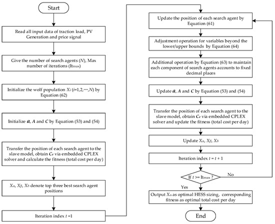
Figure 5.
Flowchart of GWO with CPLEX solver embedded.
6. Case Study
To validate the feasibility of proposed HESS sizing approach, an HSR line with a length of 710 km at the design phase in Xinjiang province is considered for case study. In this section the total cost of different cases within the project service period are compared and the effects of electricity pricing strategies, length of project service time and initial SOC of HESS are also analyzed.
6.1. Cases Description and Input Parameters
As the diurnal operation of HESS is regarded as repeated within the project service period, the simulation period for case study is one day and TSS 2 of the HSR line is selected as an example for detailed cases analysis. Four different scenarios are proposed and they are presented as follows:
- Case 1: conventional railway system with no HESS nor PV generation, as the base case;
- Case 2: conventional railway system with HESS only;
- Case 3: conventional railway system with battery energy storage systems only;
- Case 4: conventional railway system with both HESS and PV generation.
As an illustration, the longitudinal profile of considered HSR line and the location of traction substations are outlined in Figure 6. The designed maximum speed is limited at 250 km/h. It turns out that there are high altitude drops between several adjacent TSSs, which is in favor of the production of RBP.
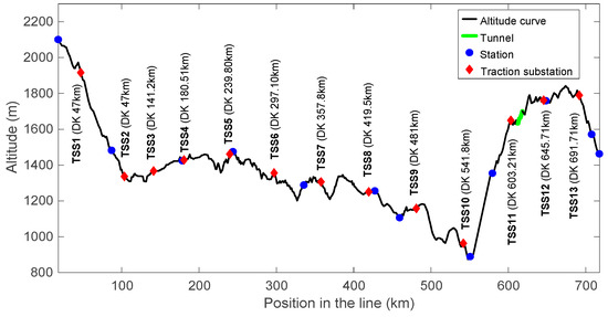
Figure 6.
Longitudinal profile of HSR line for case study.
CRH-3 HST (manufactured by China Railway Rolling Stock Corporation, Qingdao, China) is considered in this HSR line. Physical parameters of CRH-3 HST are listed in Table 1 and the traction and braking characteristics are presented in Figure 7. In regard to timetable, the departure time interval of trains is 30 min for both traveling directions. Based on the above parameters of the trains and the HSR line, the speed and power consumption of each train along the line are obtained by means of the computer simulation software WEBAnet. The simulation results of upward trains are shown in Figure 8 and downward trains are processed in the same manner.

Table 1.
Parameters of CRH-3 HST.
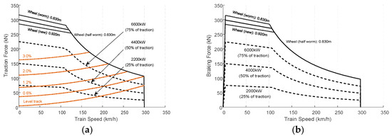
Figure 7.
Traction and braking characteristic of CRH-3 high-speed train: (a) Traction curve; (b) Braking curve.
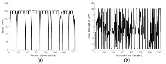
Figure 8.
Dynamic speed and power consumption of upward trains versus position: (a) Speed curve; (b) Energy consumption curve, where the negative values indicate regenerative braking power.
For the utilization of RES, PV generation sources are included in RESEM system. It is assumed that PV generation sources are connected to the traction substations. As for PV panels, ηpv = 12%, Apv = 104 m2. PV converter capacity Spv = 1 MVA. The annual profile of solar irradiance can be obtained from [56] and four representative scenarios after using forward reduction algorithm are illustrated in Figure 9b.
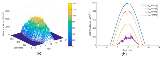
Figure 9.
Initial and reduced scenarios: (a) Annual data of solar irradiance; (b) Typical scenarios of solar irradiance after scenario reduction.
With regard to HESS, lead-acid (LA) batteries and UCs are considered in this study. All parameters associated with HESS are presented in Table 2 [31,32,47,57]. It is assumed that the service period of this project is 20 years and all the HESS-related devices can serve for the entire project period except for batteries. The lifetime estimation of LA batteries can be obtained according to the method introduced in previous sections.
Table 2.
Parameters of hybrid energy storage systems.
Two different electricity pricing schemes, including fixed tariff and time-of-use (TOU) tariff are considered here. The fixed tariff is 0.782 CNY/kWh for all time periods. As for TOU tariff, electricity price varies at different time periods. The price is 1.252 CNY/kWh for peak time periods of 8:00–11:00 and 18:00–21:00, 0.370 CNY/kWh for valley time periods of 0:00–6:00 and 22:00–0:00, 0.782 CNY/kWh for the rest time periods. The penalty charge price equals to the electricity price. Moreover, the demand charge price is 1.2 CNY/kW and the annual discount rate r0 is 5%. It is assumed that the upper and lower bounds of decision variables of master level model are MW, MWh, MW and MWh. The GWO with CPLEX solver embedded approach is implemented under a MATLAB environment on a computer with Intel Core i5-4210M CPU at 2.6 GHz and 8 GB RAM. In GWO the number of search agents is 50 and the maximum number of iterations is 50. CPLEX solver is performed with YALMIP toolbox [58] for the convenience of describing variables and constraints easily and selecting different solvers.
6.2. Cases Results Analysis
6.2.1. Case 1
As the base case, Case 1 demonstrates the scenario of conventional railway system at present, i.e., no HESS, RES considered. Toward this end, the total cost per day equals to the daily electricity cost. The results are listed in Table 3 and the composition of electricity cost is presented in Figure 10.
Table 3.
Results of different cases.
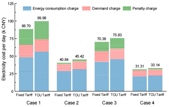
Figure 10.
Electricity cost and composition in different cases.
The obtained results are 88.70 k CNY and 99.98 k CNY under fixed tariff and TOU tariff respectively. It shows that rail operators can benefit more under fixed tariff from the perspective of daily cost, which is in line with current situation that fixed tariff is adopted in Chinese railway systems.
6.2.2. Case 2
In this case, HESS is included compared to Case 1. By applying proposed bi-level model combining HESS sizing and daily scheduling, the optimized sizing results are shown in Table 3. It is interesting that there are electricity cost savings of 53.96% under fixed tariff and 54.57% under TOU tariff, and the corresponding percentage for total cost saving are 21.78% and 24.12%, owing to the operation of charging at valley time period with low price and discharging at peak time period with high price under TOU tariff.
Another significant difference we need to pay close attention to is the battery lifetime. As shown in Table 3, the battery lifetime of 3.26 years under TOU tariff is apparently shorter than that of 5.27 years under fixed tariff, primarily arising from the fact that battery performs with a broader range of SOC and larger DOD of cycles so as to take advantage of the pricing signal and minimize the electricity cost under TOU tariff.
In order to demonstrate the operation status of system components in detail, a time horizon of 2 h and a half from 8:00 to 10:30 is highlighted, as shown in Figure 11. As we can observe from Figure 10a, the effects of peak traction load shaving and RBP absorption are significant with the application of HESS compared to case 1, which gives an explicit explanation of the remarkable reduction of electricity cost. The frequent energizing of UC and relatively smooth energizing of LA battery depicted in Figure 11b,c reveal that, UC takes the responsibility of responding to power peaks rapidly, while LA battery plays the role of storing massive energy.
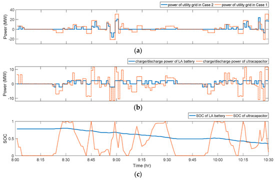
Figure 11.
Results demonstration of Case 1 and Case 2: (a) Power of utility grid in Case 1 and Case 2, where positive values indicate power imported from grid and negative values indicate power fed back to grid; (b) Charge and discharge power of LA battery and UC in Case 2, where positive values indicate discharge power and negative values indicate charge power; (c) SOC of LA battery and UC in Case 2.
6.2.3. Case 3
In this section we consider the base case with BESS, for the comparison with the performance of HESS. All parameters of LA battery are same with HESS in Case 2. The power and SOC of LA battery during a time horizon of 2 h and a half are illustrated in Figure 12.
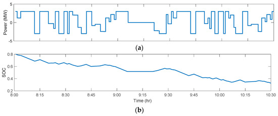
Figure 12.
Power and SOC of LA battery in Case 3 under TOU tariff: (a) Charge and discharge power, where positive values indicate discharge power and negative values indicate charge power; (b) SOC.
As we can observe from Table 3, battery lifetime are 1.21 year and 1.10 year under fixed tariff and TOU tariff in case 3, which is much shorter than that in case 2, and the replacement cost in Case 3 is consequently much larger than that in Case 2. Moreover, negative total cost savings of −10.86% and −1.31% under these two pricing schemes are achieved, which means that the daily total cost is even larger than initial electricity cost in Case 1. In order to explain the difference of battery lifetime in detail, the SOC curve of LA battery in Case 2 and Case 3 are illustrated in Figure 12.
As Figure 13 shows, the SOC curve of LA battery in Case 3 contains more fluctuating components and micro-cycles. For instance, in Figure 13a, SOC of LA battery in Case 2 contains merely a half cycle in a fixed time horizon of two hours. By contrast, SOC of LA battery in Case 3 has five half cycles and seven full cycles, resulting in a significant reduction of battery lifetime and degradation of system applicability. As a result, compared to BESS, a combination of battery and UC cannot only perform in a more flexible manner, but also help prolong the battery lifetime and reduce relevant replacement cost.
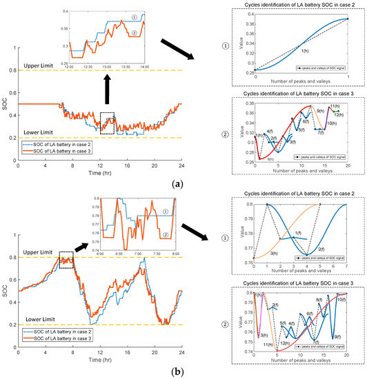
Figure 13.
SOC curve of LA battery and cycle identification in Case 2 (HESS) and Case 3 (BESS): (a) Under fixed tariff; (b) Under TOU tariff, where (f) denotes full cycle and (h) denotes a half cycle.
6.2.4. Case 4
For the utilization of renewable energy sources, PV generation as well as HESS are included in this case. The power and SOC of LA battery and UC over a time horizon of 2 h and a half are presented in Figure 14. The obtained results show that there are 27.07% and 32.39% of total cost savings under two price schemes, with marked improvements compared to Case 2.
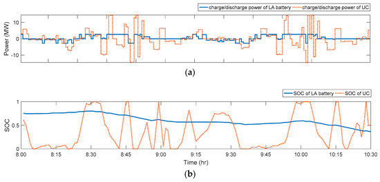
Figure 14.
Power and SOC of LA battery and UC in Case 4 under TOU tariff: (a) Charge and discharge power, where positive values indicate discharge power and negative values indicate charge power; (b) SOC.
However, it is noteworthy that the battery lifetimes of 3.95 and 2.84 years in this case are evidently decreased compared to the 5.47 and 3.26 years in Case 2. As shown in Figure 15, the difference of LA battery SOC with or without PV integrated occurs at the daytime, particularly from 10:00 to 18:00. Generally, at daytime LA battery SOC curve in Case 4 stays at a higher level, while contains more cycles with larger DOD.
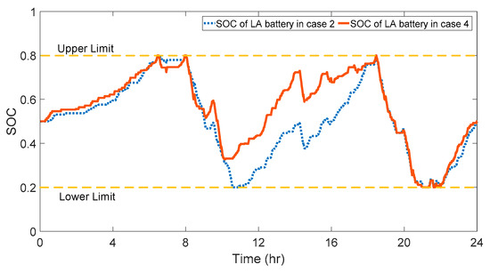
Figure 15.
Comparison of LA battery SOC between Case 2 (without PV integrated) and Case 4 in scenario 2 (with integrated PV).
As PV generation is considered here, batteries tend to charge and discharge more frequently to make full use of the available renewable energy and reduce the energy demand from utility grid so as to reduce the electricity cost, which inevitably accelerates the aging of batteries.
6.2.5. Convergence Performance of GWO
As GWO algorithm is utilized to solve the master level problem, a comparison of convergence performance between GWO, differential evolution (DE), simulated annealing (SA) optimization and particle swarm optimization (PSO) is conducted, as shown in Figure 16. Note that in this section, these four algorithms with embedded CPLEX solver are used to solve the problem in Case 2 under fixed tariff.
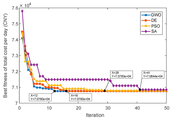
Figure 16.
Convergence characteristics of grey wolf optimizer, differential evolution, simulated annealing optimization and particle swarm optimization for Case 2 under fixed tariff.
Figure 16 shows that the optimal solution of GWO equals to that of DE (70.760 k), both of which are better than PSO (70.783 k) and SA (70.844 k). Besides, the optimal solutions of GWO, DE, PSO and SA are achieved at the 12th, 16th, 29th and 41th iterations, respectively, which indicates that GWO algorithm has better convergence performance than the other algorithms for solving the RTSEM problem in this paper. Therefore, the results validate the effectiveness of GWO technique with embedded CPLEX solver.
6.3. Sensitivities Analysis
As the default project service period and daily initial SOC of HESS are set as 20 years and 50% in previous cases analysis, in this section, the sensitivities analysis concerning daily initial SOC of HESS and project service period are performed to evaluate the impact of these two parameters on total cost savings.
As for the sensitivity analysis concerning daily initial SOC of HESS, both LA battery and UC are performed with the same initial SOC so that the considered initial SOC depends on the SOC range of LA battery. A series of initial SOC values of 20%, 30%, 40%, 50%, 60%, 70% and 80% are simulated with default project service period under fixed price tariff and relevant results are shown in Figure 17a. As observed in Figure 17a, a maximum total cost saving of 20.22% is achieved with initial SOC of 50%, as a result of allowing for a more flexible SOC range.
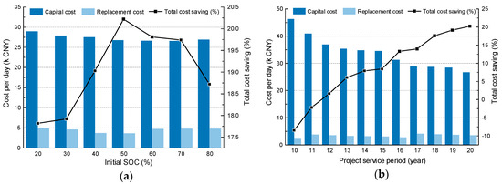
Figure 17.
Sensitivity studies: (a) The impact of initial SOC of HESS on total cost saving; (b) The impact of project service period on total cost saving.
With regard to the project service period, a series of integers from 10 to 20 years are considered for sensitivity study with default initial SOC. Figure 17b reveals that total cost savings keep increasing with the extension of project service period, arising from a more sufficient utilization of UC. It’s worth noting that the project period should be bounded by the UC cycle lifetime.
6.4. Cost Savings Analysis of TSSs in the HSR Line
Detailed case studies of TSS 2 have been performed in the previous sections. Here we concentrate on the cost-saving study of remaining TSSs in the HSR line and try to evaluate whether each TSS shows satisfactory cost-saving potentials when the HESS is integrated. Note that one of the two power supply sections that each TSS contains is selected for cost savings analysis.
As observed from Figure 18, almost all TSSs shows different levels of economic-saving potentials and the best cost saving is achieved at TSS 10, primarily arising from considerable RBP of train at on long and sharp grade. With regard to TSS 12 and TSS 13, high altitude and relatively gentle sloping track result in lower RBP for reuse and inconspicuous cost-saving results. Toward this end, TSSs with notable cost savings should be given priority to when HESS is applied in the future.
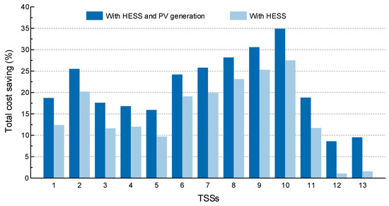
Figure 18.
Cost saving results of TSSs in the HSR line.
7. Conclusions
This paper proposes a bi-level model combining long-term HESS sizing and short-term diurnal HESS dispatch strategy for energy management in railway traction substations. The optimized sizing of HESS involving power rating and capacity of LA battery and UC is formulated in the master level model with the intention of minimizing the total cost throughout the project service period, with battery degradation and replacement cost taken into account. While the diurnal HESS scheduling strategy is formulated as a MILP model in the slave level model. The proposed GWO with CPLEX solver embedded approach has been implemented successfully on TSSs of considered HSR line. The case study results reveal that there are significant cost savings with the integration of HESS and RES under both fixed tariff (25.5%) and TOU tariff (30.95%). Besides, a combination of battery and UC, namely HESS, helps prolong the battery lifetime and reduce replacement cost remarkably. Meanwhile, the daily initial SOC of HESS and project service period are found to have significant impacts on total cost savings, and the sensitivity analysis is performed. It is noteworthy that TSSs in the HSR line present different cost-saving potentials under different line geometry, thus it is crucial to evaluate each TSS in advance so as to provide preferences for further application of HESS.
Future work can incorporate the power flow calculation of traction networks into the optimization model and figure out the optimal position and sizing of HESS and RES in the HSR line. Moreover, HESS between adjacent power supply sections for power routing and negative sequence reduction deserves further study.
Author Contributions
Y.L. and M.C. proposed the idea, developed the model, performed the simulation works and wrote the paper. S.L., Y.C. were in charge of review and editing. This work was conducted under the supervision of Q.L.
Funding
This research was funded by the National Natural Science Foundation of China (Grant No. 51877182) and the Science and Technology Plan Project of Sichuan Province (Grant No. 2018FZ0107). The APC was funded by the National Natural Science Foundation of China and the Science and Technology Plan Project of Sichuan Province.
Acknowledgments
This research was supported by the China Railway Construction Co., Ltd. (CRCC) and the First Design and Survey Institute (FDSI) Group Co., Ltd.
Conflicts of Interest
The authors declare no conflict of interest.
Nomenclature
| Abbreviations | |
| RTSEM | Railway traction substation energy management |
| HESS | Hybrid Energy storage systems |
| PCS | Power conversion systems |
| BOP | Balance of plant |
| RBP | Regenerative braking power |
| UC | Ultracapacitor |
| LA | Lead-acid |
| PV | Photovoltaic |
| MILP | Mixed-integer linear programming |
| HSR | High-speed railway |
| HSTs | High-speed trains |
| DOD | Depth of discharge |
| SOC | State of charge |
| Parameters | |
| Railway traction load at time interval t (MW) | |
| Regenerative braking power at time interval t (MW) | |
| T | Total number of operation time intervals during a day |
| ∆t | The discretization time interval (1 min) |
| Electricity price for power imported from the utility grid (CNY/MWh) | |
| penalty charge for power fed back to the utility grid (CNY/MWh) | |
| Total area of PV panels (m2) | |
| Probability of PV generation scenario | |
| Solar irradiance at time interval t for scenario s (kW/m2) | |
| Tproj | Project service period (year) |
| r0 | Annual discount rate |
| , | Upper and lower bounds of power rating of battery (MW) |
| , | Upper and lower bounds of capacity of battery (MWh) |
| , | Upper and lower bounds of power rating of UC (MW) |
| , | Upper and lower bounds of capacity of UC (MWh) |
| , | Discharge and charge efficiency of battery |
| , | Discharge and charge efficiency of UC |
| , | Self-discharging rate of battery and UC |
| , | Minimum and maximum SOC limit of battery |
| Initial SOC of battery per day | |
| , | Minimum and maximum SOC limit of UC |
| Initial SOC of UC per day | |
| Maximum limit for active power imported from the utility grid (MW) | |
| Maximum limit for regenerative braking power fed back to the utility grid (MW) | |
| Variables | |
| , | Discharge and charge power of battery at time interval t for scenario s (MW) |
| , | Discharge and charge power of UC at time interval t for scenario s (MW) |
| Power supplied by the utility grid at time interval t for scenario s (MW) | |
| Power fed back to utility grid at time interval t for scenario s (MW) | |
| PV output power at time interval t for scenario s (MW) | |
| , | The energy stored in battery and UC at time interval t for scenario s (MWh) |
| , | Binary variable: 1 if battery or UC are discharging at time interval t for scenario s, 0 otherwise |
| , | Binary variable: 1 if battery or UC are charging at time interval t for scenario s, 0 otherwise |
| , | Binary variable: 1 if battery or UC are in operation mode (charge/discharge) at time interval t for scenario s, 0 otherwise |
| Binary variable: 1 if grid supplies power to trains, and 0 if braking power is fed back to grid. | |
| Battery lifetime (year), as an intermediate variable | |
| , | Rated power of battery and UC (MW) |
| , | Rated capacity of battery and UC (MWh) |
| , | Operation time of battery and UC per day (hour), as intermediate variables |
References
- Intergovernmental Panel on Climate Change. Climate Change 2014—Impacts, Adaptation and Vulnerability Part A: Global and Sectoral Aspects; Cambridge University Press: Cambridge, UK; New York, NY, USA, 2014; ISBN 1-107-05807-4. [Google Scholar]
- Intergovernmental Panel on Climate Change. Climate Change 2014—Impacts, Adaptation and Vulnerability Part B: Regional Aspects; Cambridge University Press: Cambridge, UK; New York, NY, USA, 2014; ISBN 1-107-05816-3. [Google Scholar]
- Kyoto Protocol to the United Nations Framework Convention on Climate Change. Available online: https://unfccc.int/process/the-kyoto-protocol (accessed on 11 February 2018).
- Doha Amendment to the Kyoto Protocol. Available online: https://unfccc.int/process/the-kyoto-protocol/the-doha-amendment (accessed on 11 February 2018).
- Yan, Q.; Wang, Y.; Baležentis, T.; Sun, Y.; Streimikiene, D. Energy-Related CO2 Emission in China’s Provincial Thermal Electricity Generation: Driving Factors and Possibilities for Abatement. Energies 2018, 11, 1096. [Google Scholar] [CrossRef]
- Railway Handbook 2017: Energy Consumption and CO2 Emissions. Available online: https://uic.org/IMG/pdf/handbook_iea-uic_2017_web2-2.pdf (accessed on 2 February 2018).
- Wang, K.; Hu, H.; Zheng, Z.; He, Z.; Chen, L. Study on Power Factor Behavior in High-Speed Railways Considering Train Timetable. IEEE Trans. Transp. Electrif. 2018, 4, 220–231. [Google Scholar] [CrossRef]
- Ratniyomchai, T.; Hillmansen, S.; Tricoli, P. Recent developments and applications of energy storage devices in electrified railways. IET Electr. Syst. Transp. 2014, 4, 9–20. [Google Scholar] [CrossRef]
- Sitras SES of Siemens Transportation Systems: Energy Storage System for Mass Transit Systems. Available online: https://w3.usa.siemens.com/mobility/us/Documents/en/rail-solutions/railway-electrification/dc-traction-power-supply/sitras-ses2-en.pdf (accessed on 15 January 2018).
- MITRAC Energy Saver. Available online: https://www.bombardier.com/en/media/insight/economy-and-rail/eco4-technologies/mitrac-energy-saver.html (accessed on 15 January 2018).
- Moskowitz, J.P.; Cohuau, J.L. STEEM: ALSTOM and RATP experience of supercapacitors in tramway operation. In Proceedings of the 2010 IEEE Vehicle Power and Propulsion Conference, Lille, France, 1–3 September 2010; pp. 1–5. [Google Scholar]
- Shu, Z.; Xie, S.; Li, Q. Single-Phase Back-To-Back Converter for Active Power Balancing, Reactive Power Compensation, and Harmonic Filtering in Traction Power System. IEEE Trans. Power Electron. 2011, 26, 334–343. [Google Scholar] [CrossRef]
- Riffonneau, Y.; Bacha, S.; Barruel, F.; Ploix, S. Optimal Power Flow Management for Grid Connected PV Systems with Batteries. IEEE Trans. Sustain. Energy 2011, 2, 309–320. [Google Scholar] [CrossRef]
- Roncero-Sánchez, P.; Parreño Torres, A.; Vázquez, J. Control Scheme of a Concentration Photovoltaic Plant with a Hybrid Energy Storage System Connected to the Grid. Energies 2018, 11, 301. [Google Scholar] [CrossRef]
- Jiang, Q.; Gong, Y.; Wang, H. A Battery Energy Storage System Dual-Layer Control Strategy for Mitigating Wind Farm Fluctuations. IEEE Trans. Power Syst. 2013, 28, 3263–3273. [Google Scholar] [CrossRef]
- Li, R.; Wang, W.; Chen, Z.; Wu, X. Optimal planning of energy storage system in active distribution system based on fuzzy multi-objective bi-level optimization. J. Mod. Power Syst. Clean Energy 2018, 6, 342–355. [Google Scholar] [CrossRef]
- Fossati, J.P.; Galarza, A.; Martín-Villate, A.; Fontán, L. A method for optimal sizing energy storage systems for microgrids. Renew. Energy 2015, 77, 539–549. [Google Scholar] [CrossRef]
- Sukumar, S.; Mokhlis, H.; Mekhilef, S.; Naidu, K.; Karimi, M. Mix-mode energy management strategy and battery sizing for economic operation of grid-tied microgrid. Energy 2017, 118, 1322–1333. [Google Scholar] [CrossRef]
- Chen, C.; Duan, S.; Cai, T.; Liu, B.; Hu, G. Optimal Allocation and Economic Analysis of Energy Storage System in Microgrids. IEEE Trans. Power Electron. 2011, 26, 2762–2773. [Google Scholar] [CrossRef]
- Akram, U.; Khalid, M.; Shafiq, S. Optimal sizing of a wind/solar/battery hybrid grid-connected microgrid system. IET Renew. Power Gener. 2017, 12, 72–80. [Google Scholar] [CrossRef]
- Serpi, A.; Porru, M.; Damiano, A. An Optimal Power and Energy Management by Hybrid Energy Storage Systems in Microgrids. Energies 2017, 10, 1909. [Google Scholar] [CrossRef]
- Wang, H.; Wang, T.; Xie, X.; Ling, Z.; Gao, G.; Dong, X. Optimal Capacity Configuration of a Hybrid Energy Storage System for an Isolated Microgrid Using Quantum-Behaved Particle Swarm Optimization. Energies 2018, 11, 454. [Google Scholar] [CrossRef]
- Khayyam, S.; Ponci, F.; Goikoetxea, J.; Recagno, V.; Bagliano, V.; Monti, A. Railway Energy Management System: Centralized–Decentralized Automation Architecture. IEEE Trans. Smart Grid 2016, 7, 1164–1175. [Google Scholar] [CrossRef]
- Pankovits, P.; Ployard, M.; Pouget, J.; Brisset, S.; Abbes, D.; Robyns, B. Design and operation optimization of a hybrid railway power substation. In Proceedings of the 2013 15th European Conference on Power Electronics and Applications (EPE), Lille, France, 2–6 September 2013; pp. 1–8. [Google Scholar]
- Pankovits, P.; Abbes, D.; Saudemont, C.; Abdou, O.M.; Pouget, J.; Robyns, B. Energy management multi-criteria design for hybrid railway power substations. In Proceedings of the 11th International Conference on Modeling and Simulation of Electric Machines, Converters and Systems (Electrimacs 2014), Valencia, Spain, 20–22 May 2014. [Google Scholar]
- Pankovits, P.; Pouget, J.; Robyns, B.; Delhaye, F.; Brisset, S. Towards railway-smartgrid: Energy management optimization for hybrid railway power substations. In Proceedings of the IEEE PES Innovative Smart Grid Technologies, Europe, Istanbul, Turkey, 12–15 October 2014; pp. 1–6. [Google Scholar]
- Novak, H.; Vašak, M.; Lešić, V. Hierarchical energy management of multi-train railway transport system with energy storages. In Proceedings of the IEEE International Conference on Intelligent Rail Transportation (ICIRT), Birmingham, UK, 23–25 August 2016; pp. 130–138. [Google Scholar]
- Novak, H.; Lesic, V.; Vasak, M. Hierarchical Coordination of Trains and Traction Substation Storages for Energy Cost Optimization. In Proceedings of the 2017 IEEE 20th International Conference on Intelligent Transportation Systems (ITSC), Yokohama, Japan, 16–19 October 2017. [Google Scholar]
- Sengor, I.; Kilickiran, H.C.; Akdemir, H.; Kekezoglu, B.; Erdinc, O.; Catalão, J.P.S. Energy Management of A Smart Railway Station Considering Regenerative Braking and Stochastic Behaviour of ESS and PV Generation. IEEE Trans. Sustain. Energy 2018, 9, 1041–1050. [Google Scholar] [CrossRef]
- Kim, H.; Heo, J.H.; Park, J.Y.; Yoon, Y.T. Impact of Battery Energy Storage System Operation Strategy on Power System: An Urban Railway Load Case under a Time-of-Use Tariff. Energies 2017, 10, 68. [Google Scholar] [CrossRef]
- Aguado, J.A.; Racero, A.J.S.; de la Torre, S. Optimal Operation of Electric Railways ith Renewable Energy and Electric Storage Systems. IEEE Trans. Smart Grid 2018, 9, 993–1001. [Google Scholar] [CrossRef]
- De la Torre, S.; Sanchez-Racero, A.J.; Aguado, J.A.; Reyes, M.; Martianez, O. Optimal Sizing of Energy Storage for Regenerative Braking in Electric Railway Systems. IEEE Trans. Power Syst. 2015, 30, 1492–1500. [Google Scholar] [CrossRef]
- SIGNON SINAnet and WEBAnet. Available online: http://www.elbas.de/sinanetwebanet_e.html (accessed on 8 March 2018).
- Growe-Kuska, N.; Heitsch, H.; Romisch, W. Scenario reduction and scenario tree construction for power management problems. In Proceedings of the 2003 IEEE Bologna Power Tech Conference Proceedings, Bologna, Italy, 23–26 June 2003; Volume 3, p. 7. [Google Scholar]
- Soares, J.; Canizes, B.; Ghazvini, M.A.F.; Vale, Z.; Venayagamoorthy, G.K. Two-Stage Stochastic Model Using Benders’ Decomposition for Large-Scale Energy Resource Management in Smart Grids. IEEE Trans. Ind. Appl. 2017, 53, 5905–5914. [Google Scholar] [CrossRef]
- Nasri, A.; Kazempour, S.J.; Conejo, A.J.; Ghandhari, M. Network-Constrained AC Unit Commitment under Uncertainty: A Benders’ Decomposition Approach. IEEE Trans. Power Syst. 2016, 31, 412–422. [Google Scholar] [CrossRef]
- Wu, H.; Shahidehpour, M.; Alabdulwahab, A.; Abusorrah, A. A Game Theoretic Approach to Risk-Based Optimal Bidding Strategies for Electric Vehicle Aggregators in Electricity Markets with Variable Wind Energy Resources. IEEE Trans. Sustain. Energy 2016, 7, 374–385. [Google Scholar] [CrossRef]
- Dupačová, J.; Gröwe-Kuska, N.; Römisch, W. Scenario reduction in stochastic programming. Math. Program. 2003, 95, 493–511. [Google Scholar] [CrossRef]
- Razali, N.M.M.; Hashim, A.H. Backward reduction application for minimizing wind power scenarios in stochastic programming. In Proceedings of the 2010 4th International Power Engineering and Optimization Conference (PEOCO), Shah Alam, Malaysia, 23–24 June 2010; pp. 430–434. [Google Scholar]
- Fotouhi Ghazvini, M.A.; Faria, P.; Ramos, S.; Morais, H.; Vale, Z. Incentive-based demand response programs designed by asset-light retail electricity providers for the day-ahead market. Energy 2015, 82, 786–799. [Google Scholar] [CrossRef]
- Wu, H.; Shahidehpour, M.; Alabdulwahab, A.; Abusorrah, A. Thermal Generation Flexibility with Ramping Costs and Hourly Demand Response in Stochastic Security-Constrained Scheduling of Variable Energy Sources. IEEE Trans. Power Syst. 2015, 30, 2955–2964. [Google Scholar] [CrossRef]
- Tankari, M.A.; Camara, M.B.; Dakyo, B.; Lefebvre, G. Use of Ultracapacitors and Batteries for Efficient Energy Management in Wind Diesel Hybrid System. IEEE Trans. Sustain. Energy 2013, 4, 414–424. [Google Scholar] [CrossRef]
- Bordin, C.; Anuta, H.O.; Crossland, A.; Gutierrez, I.L.; Dent, C.J.; Vigo, D. A linear programming approach for battery degradation analysis and optimization in offgrid power systems with solar energy integration. Renew. Energy 2017, 101, 417–430. [Google Scholar] [CrossRef]
- Amzallag, C.; Gerey, J.; Robert, J.; Bahuaud, J. Standardization of the rainflow counting method for fatigue analysis. Int. J. Fatigue 1994, 16, 287–293. [Google Scholar] [CrossRef]
- Layadi, T.M.; Champenois, G.; Mostefai, M.; Abbes, D. Lifetime estimation tool of lead–acid batteries for hybrid power sources design. Simul. Model. Pract. Theor. 2015, 54, 36–48. [Google Scholar] [CrossRef]
- Bindner, H.; Cronin, T.; Lundsager, P.; Manwell, J.F.; Abdulwahid, U.; Baring-Gould, I. Lifetime Modelling of Lead Acid Batteries; Risø National Laboratory: Roskilde, Denmark, 2005. [Google Scholar]
- Zakeri, B.; Syri, S. Electrical energy storage systems: A comparative life cycle cost analysis. Renew. Sustain. Energy Rev. 2015, 42, 569–596. [Google Scholar] [CrossRef]
- Tsikalakis, A.G.; Hatziargyriou, N.D. Centralized Control for Optimizing Microgrids Operation. IEEE Trans. Energy Convers. 2008, 23, 241–248. [Google Scholar] [CrossRef]
- Roch-Dupre, D.; Lopez-Lopez, A.J.; Pecharroman, R.R.; Cucala, A.P.; Fernandez-Cardador, A. Analysis of the demand charge in DC railway systems and reduction of its economic impact with Energy Storage Systems. Int. J. Electr. Power Energy Syst. 2017, 93, 459–467. [Google Scholar] [CrossRef]
- Zhao, B.; Zhang, X.; Chen, J.; Wang, C.; Guo, L. Operation Optimization of Standalone Microgrids Considering Lifetime Characteristics of Battery Energy Storage System. IEEE Trans. Sustain. Energy 2013, 4, 934–943. [Google Scholar] [CrossRef]
- Zhao, B.; Zhang, X.; Li, P.; Wang, K.; Xue, M.; Wang, C. Optimal sizing, operating strategy and operational experience of a stand-alone microgrid on Dongfushan Island. Appl. Energy 2014, 113, 1656–1666. [Google Scholar] [CrossRef]
- Chen, S.X.; Gooi, H.B.; Wang, M.Q. Sizing of Energy Storage for Microgrids. IEEE Trans. Smart Grid 2012, 3, 142–151. [Google Scholar] [CrossRef]
- Mirjalili, S.; Mirjalili, S.M.; Lewis, A. Grey Wolf Optimizer. Adv. Eng. Softw. 2014, 69, 46–61. [Google Scholar] [CrossRef]
- Sharma, S.; Bhattacharjee, S.; Bhattacharya, A. Grey wolf optimisation for optimal sizing of battery energy storage device to minimise operation cost of microgrid. IET Gener. Transm. Dis. 2016, 10, 625–637. [Google Scholar] [CrossRef]
- Hassan, Z.G.; Ezzat, M.; Abdelaziz, A.Y. Enhancement of power system operation using grey wolf optimization algorithm. In Proceedings of the 2017 Nineteenth International Middle East Power Systems Conference (MEPCON), Cairo, Egypt, 19–21 September 2017; pp. 397–402. [Google Scholar]
- National Renewable Energy Laboratory Measurement and Instrumentation Data Center (MIDC). Available online: https://midcdmz.nrel.gov/ (accessed on 28 March 2018).
- Battke, B.; Schmidt, T.S.; Grosspietsch, D.; Hoffmann, V.H. A review and probabilistic model of lifecycle costs of stationary batteries in multiple applications. Renew. Sustain. Energy Rev. 2013, 25, 240–250. [Google Scholar] [CrossRef]
- Lofberg, J. YALMIP: A toolbox for modeling and optimization in MATLAB. In Proceedings of the 2004 IEEE International Conference on Robotics and Automation (IEEE Cat. No.04CH37508), New Orleans, LA, USA, 2–4 September 2004; pp. 284–289. [Google Scholar]


© 2018 by the authors. Licensee MDPI, Basel, Switzerland. This article is an open access article distributed under the terms and conditions of the Creative Commons Attribution (CC BY) license (http://creativecommons.org/licenses/by/4.0/).