Energy Balance and Local Unsteady Loss Analysis of Flows in a Low Specific Speed Model Pump-Turbine in the Positive Slope Region on the Pump Performance Curve


Abstract
:1. Introduction
2. Methodology
3. Results and Discussions
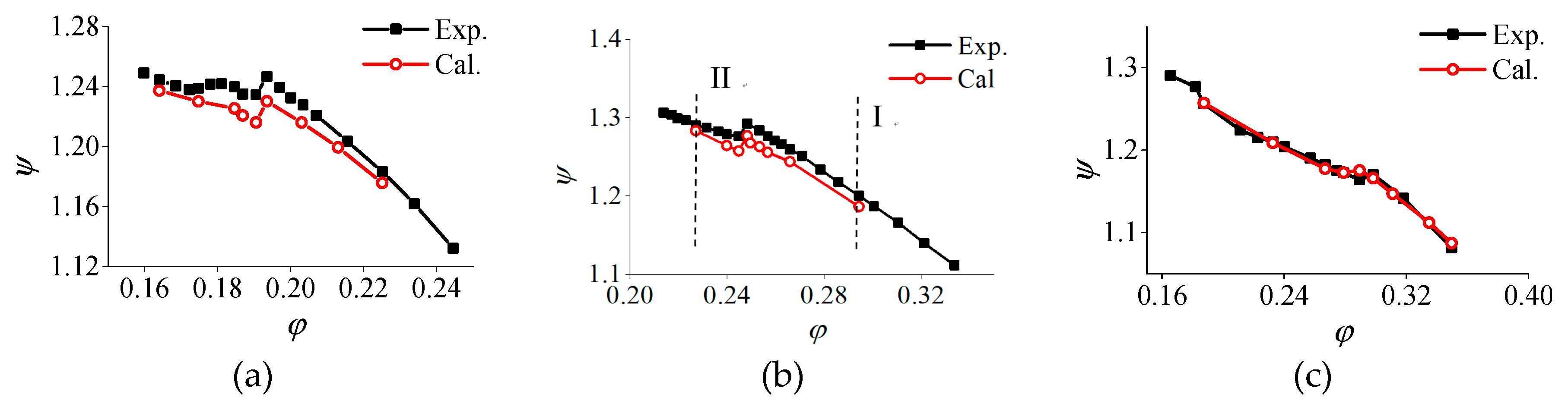
3.1. Validation of the Simulations
3.2. Pump Performance and Head Loss
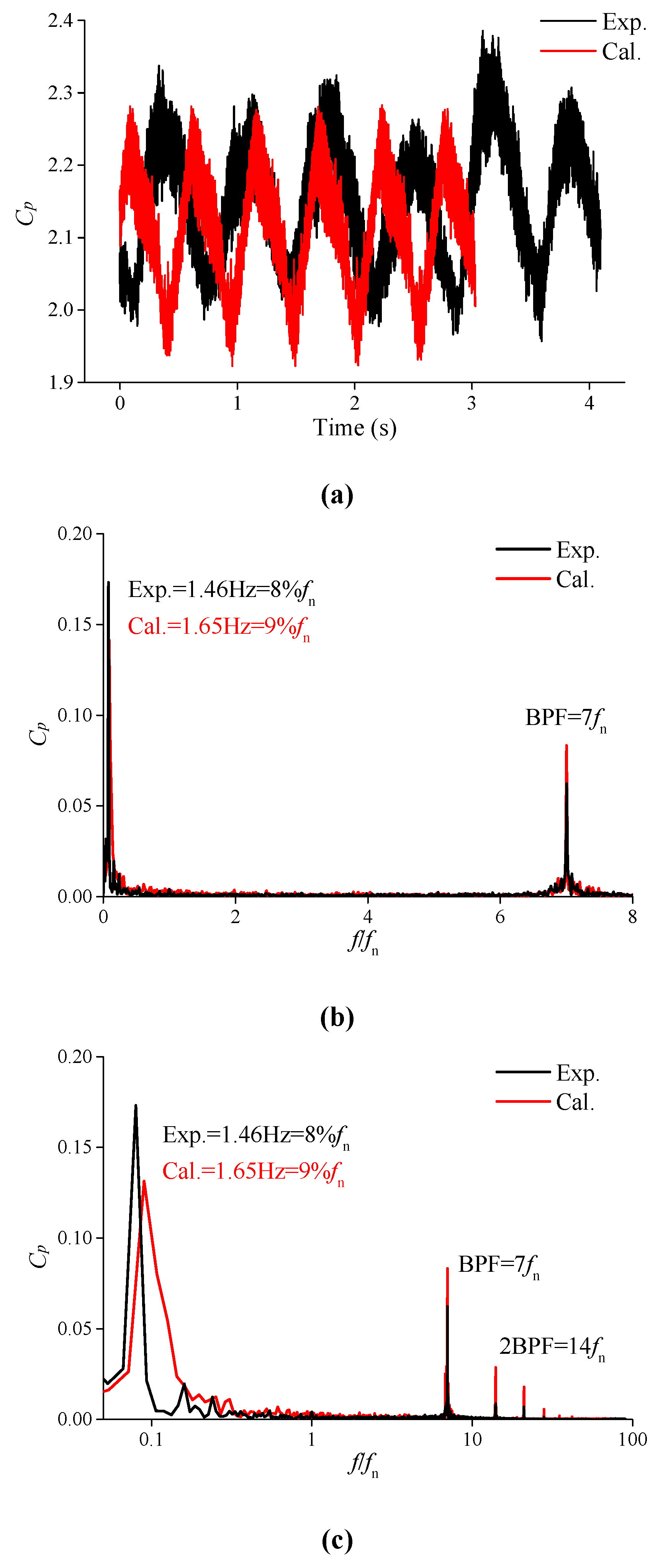
3.3. Pressure Fluctuations
3.3.1. Conditions III and IV
3.3.2. Condition V
3.4. Energy Balance Analysis
4. Analysis of the Input Power
5. Analysis of the Loss
5.1. Local Loss Analysis Method
5.2. Physical Phenomena Responsible for the Loss
5.2.1. Condition III and IV
5.2.2. Condition V
6. Concluding Remarks
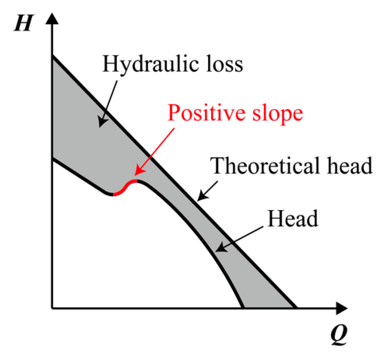
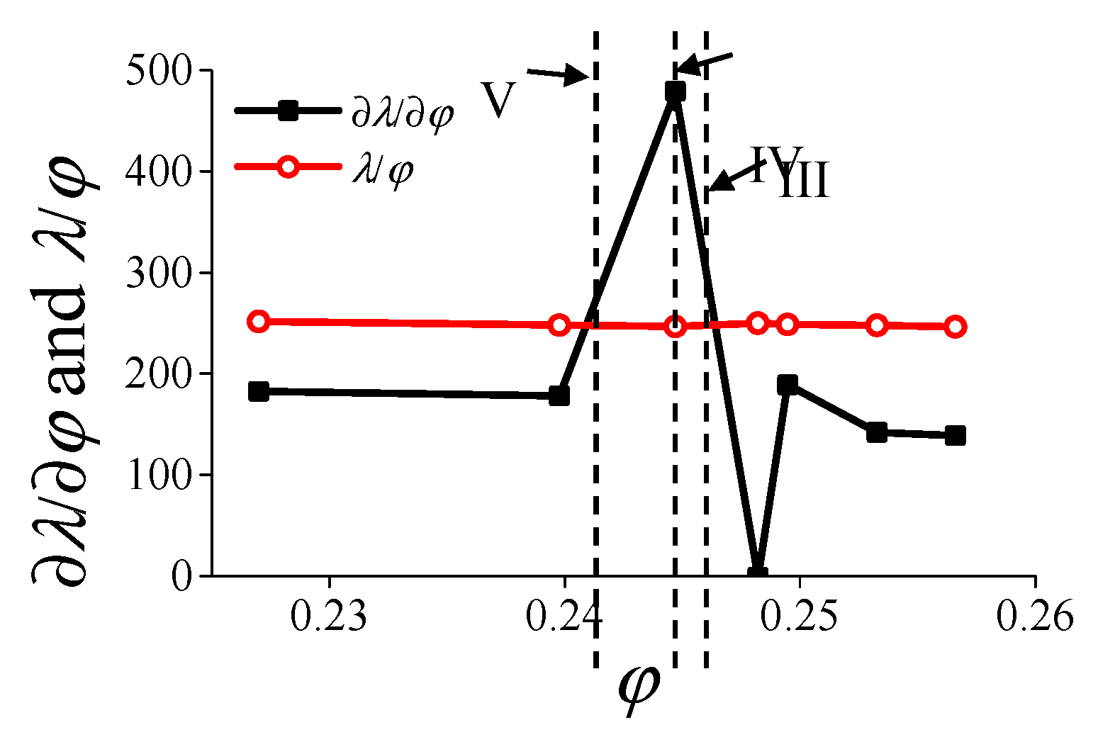
- According to the theoretical derivation, the occurrence of the positive slope on the pump performance curve corresponds to the region where is larger than a critical value . The substantial decrease of λu results in the positive slope in the pump performance curve. For this decrease of λu in the present study, about 80% is attributed to the decrease of the input power coefficient while the remaining 20% is caused the increase of the loss coefficient.
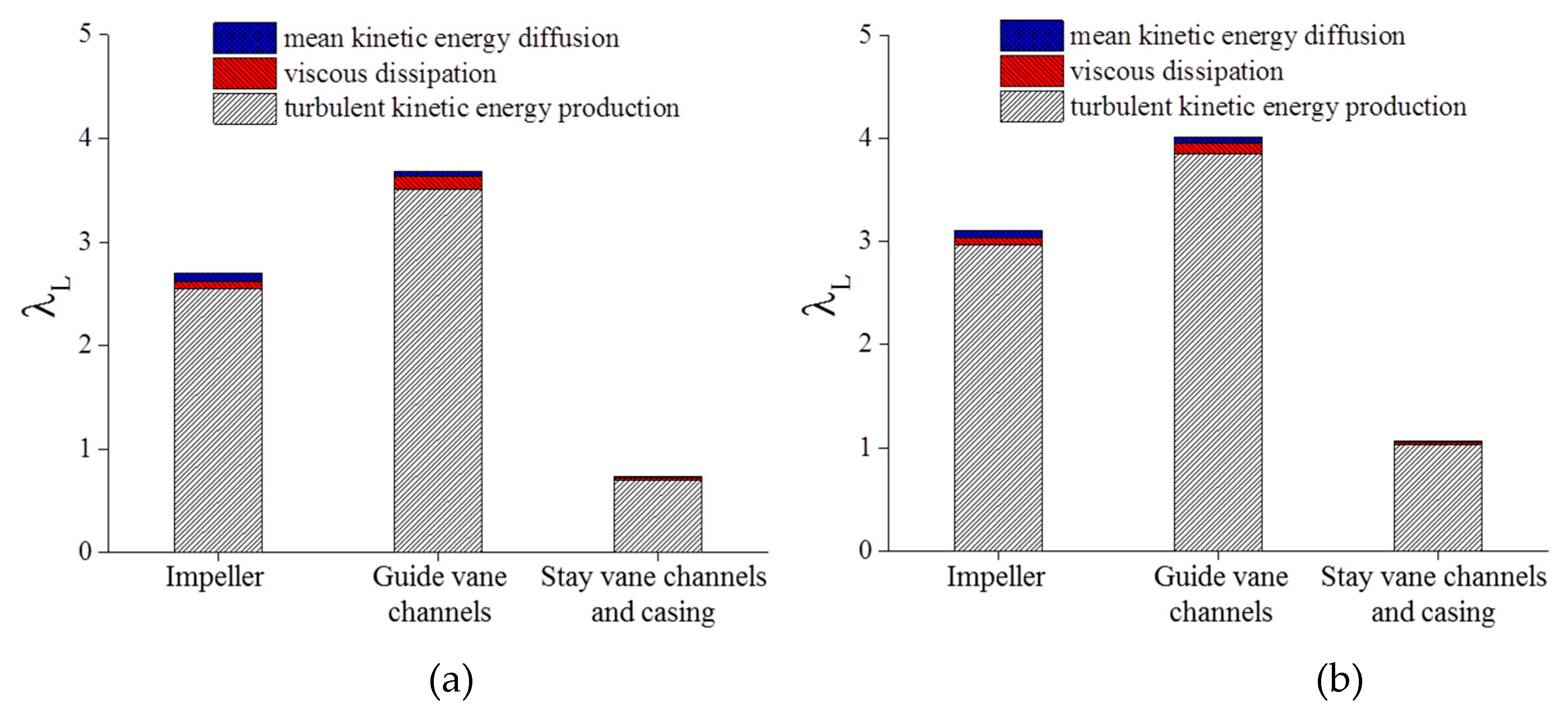
- The unsteady local loss analysis, derived from the energy equation, was conducted to illustrate the contribution of local flow patterns to the loss in corresponding hydraulic components. The variation of the kinetic energy of the mean flow was taken into account for the first time so that this method could be applied on highly time dependent flow patterns, including the rotating stall in the present study.
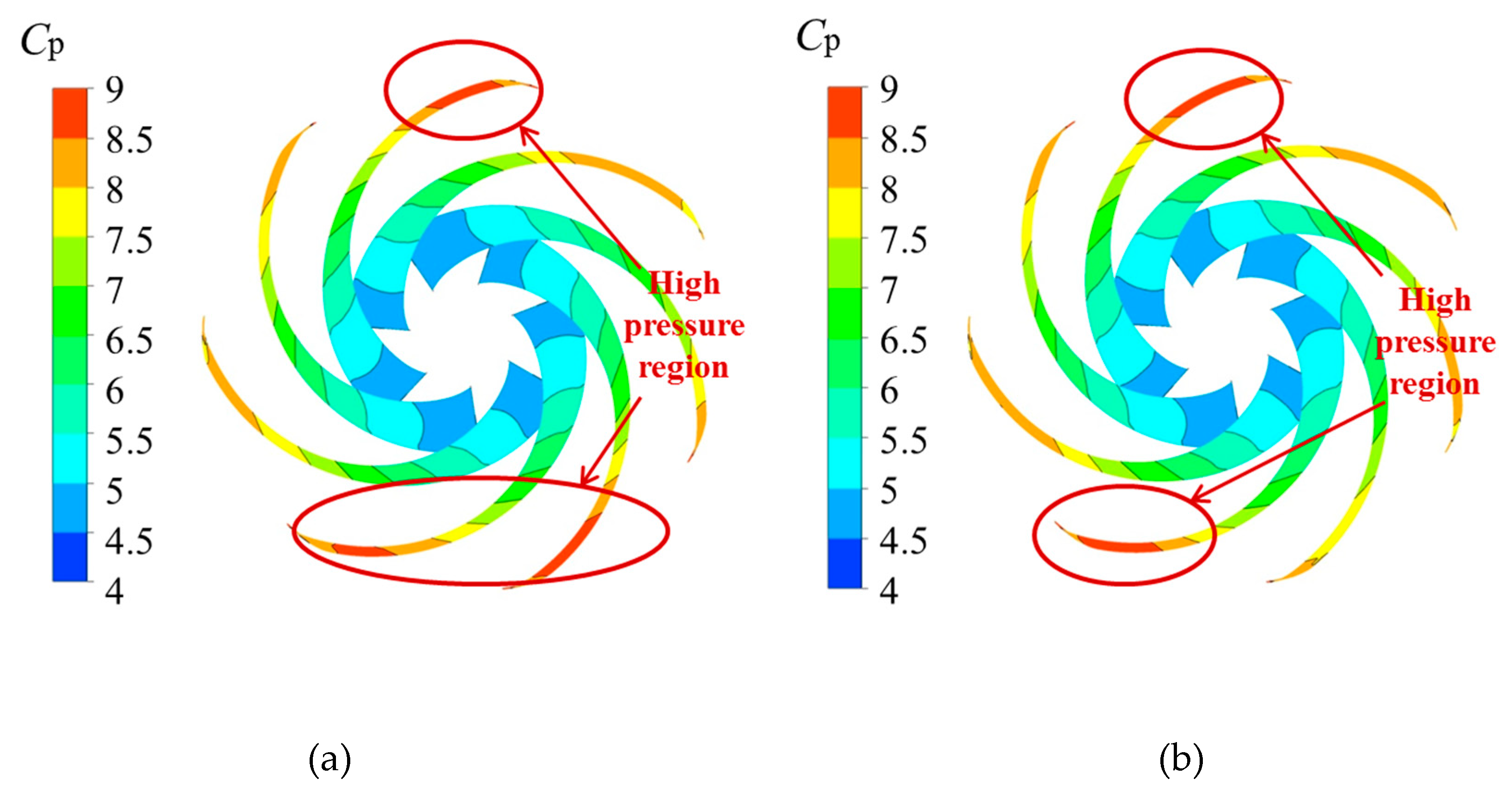
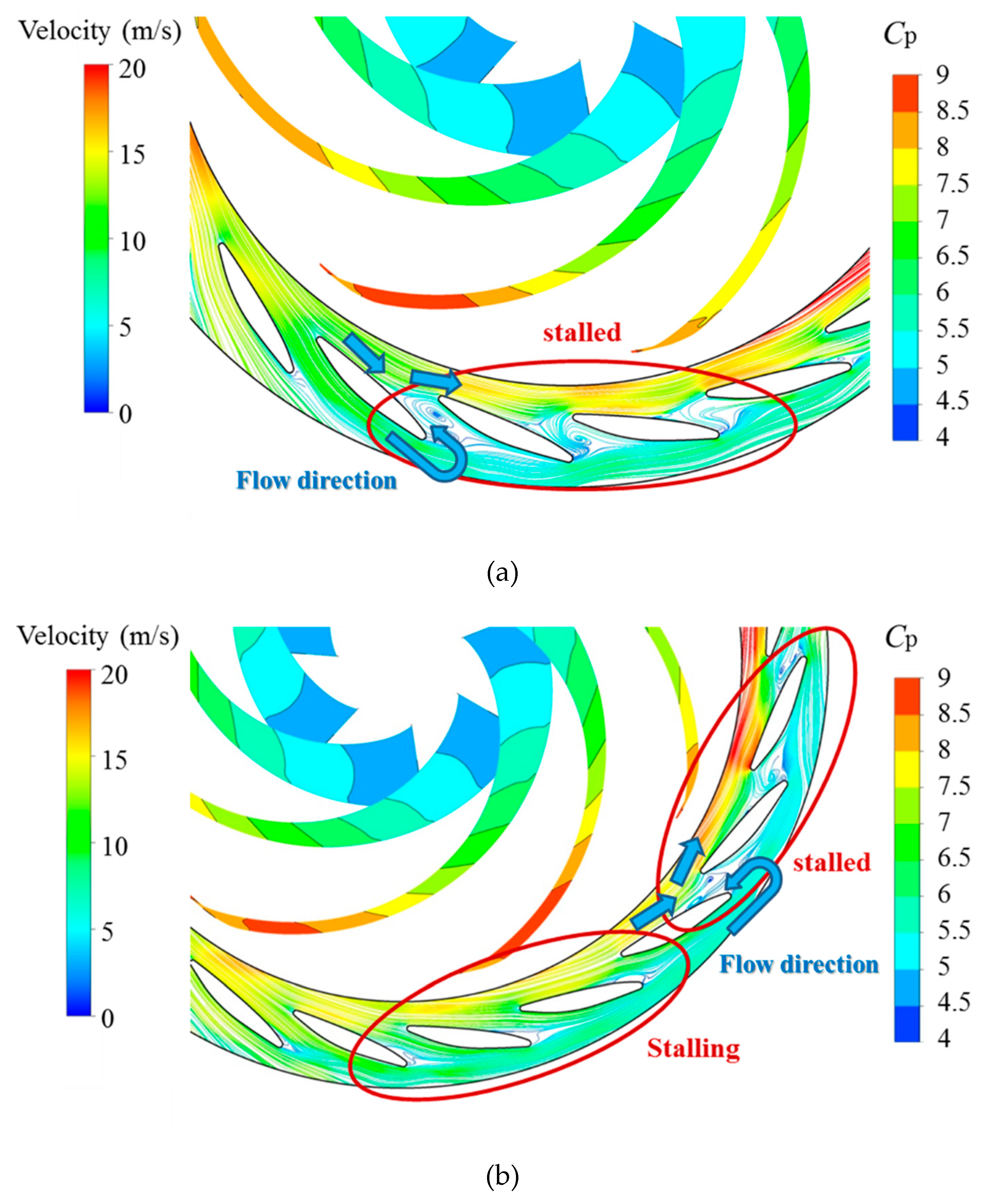
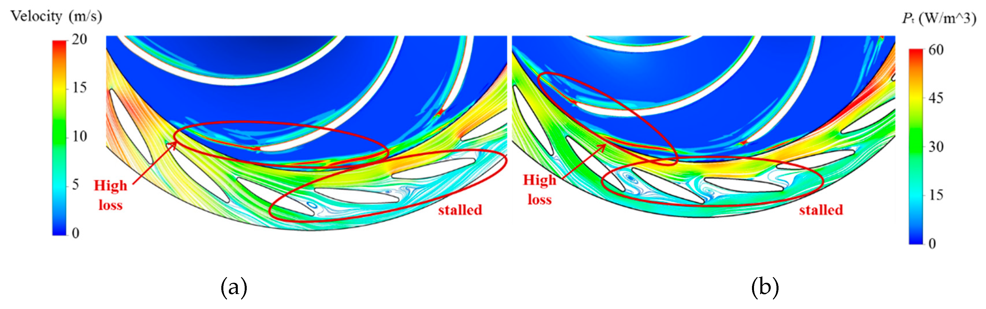
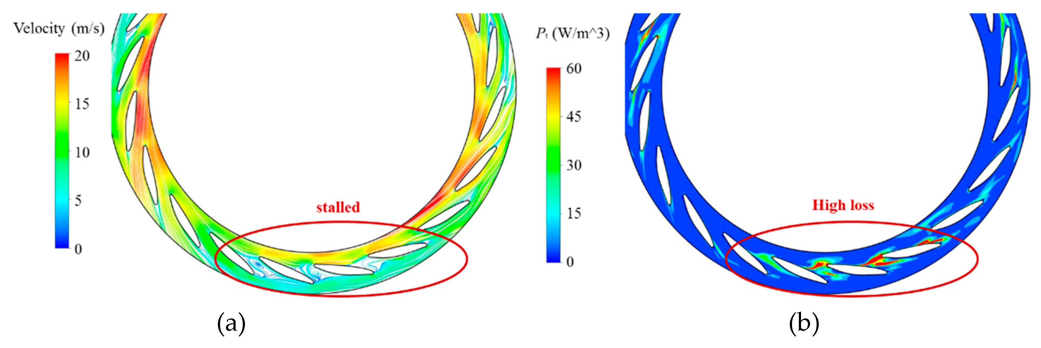
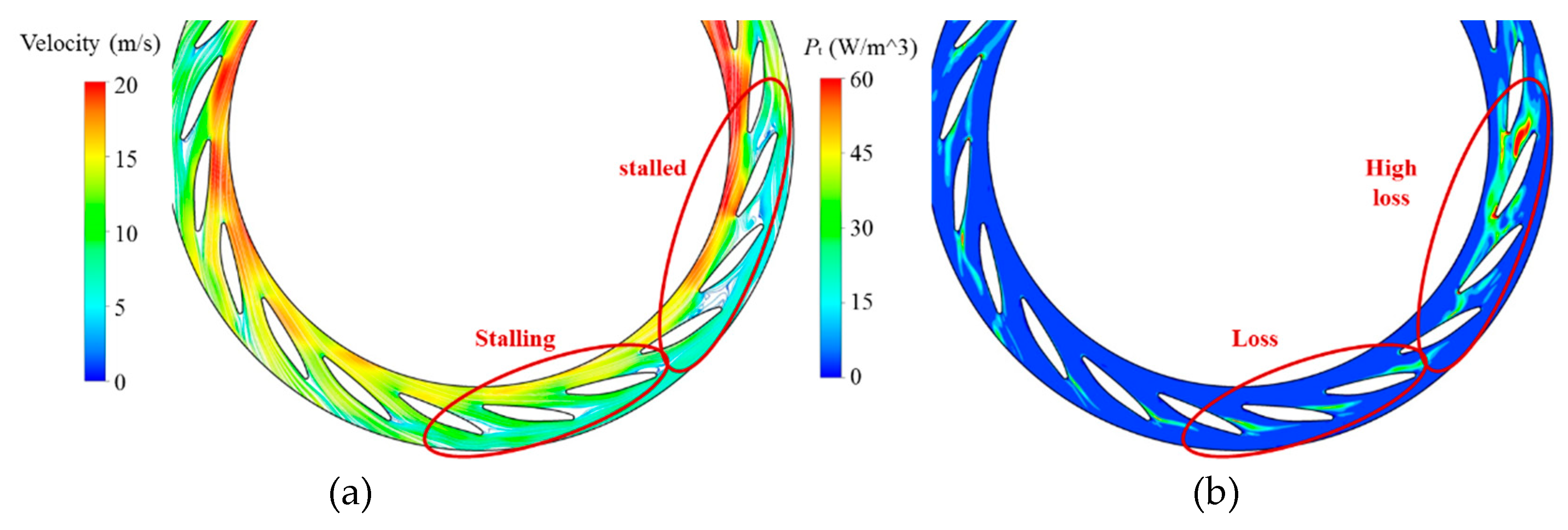
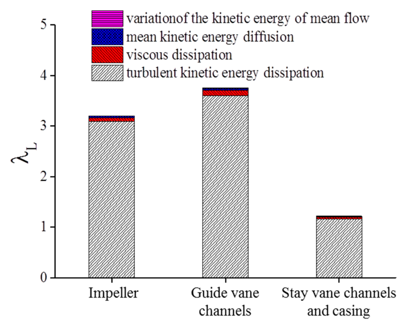
- The local loss analysis reveals that, the majority of the loss converts to the turbulent kinetic energy in the pump-turbine. The regions between the straight flow with high flow velocity and the separated flow with low flow velocity have great contributions to the loss, due to the strong velocity gradient.
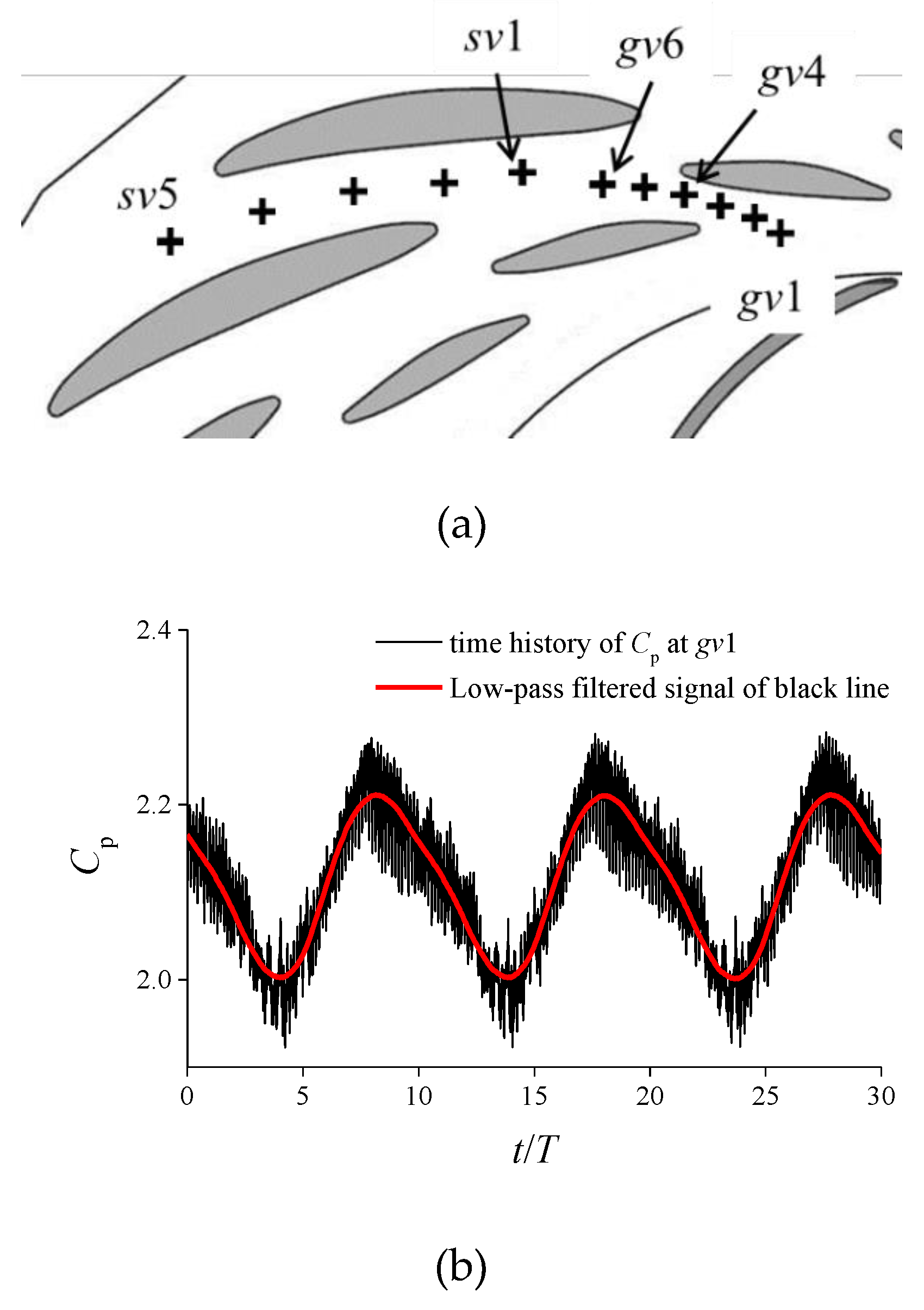
- Some guide vane channels were stalled at the condition with larger discharge coefficient than the positive slope region. Then several guide vane channels near the stalled channels were stalling with minor decrease of the discharge coefficient, leading to sudden increases of the input power and the loss. When the discharge coefficient slightly decreased in further, the pump-turbine operated into the positive slope and the rotating stall with 3 stall cells appeared, proven by the FFT and cross-phase analysis on pressure fluctuations.
Author Contributions
Acknowledgments
Conflicts of Interest
References
- Braun, O. Part Load Flow in Radial Centrifugal Pumps. Ph.D. Thesis, École Polytechnique Fédérale de Lausanne, Lausanne, Switzerland, 2009. [Google Scholar]
- Mei, Z.Y. Technology of Pumped Storage Power Generation; China Machine Press: Beijing, China, 2000. (In Chinese) [Google Scholar]
- Hasmatuchi, V. Hydrodynamics of a Pump-Turbine Operating at Off-Design Conditions in Generating Mode. Ph.D. Thesis, École Polytechnique Fédérale de Lausanne, Lausanne, Switzerland, 2012. [Google Scholar]
- Zuo, Z.G.; Liu, S.H. Flow-Induced Instabilities in Pump-Turbines in China. Engineering 2017, 3, 504–511. [Google Scholar] [CrossRef]
- Gülich, J.F. Centrifugal Pumps; Springer: Berlin, Germany, 2008. [Google Scholar]
- Eisele, K.; Muggli, F.; Zhang, Z.; Casey, M.; Sallaberger, M. Experimental and numerical studies of flow instabilities in pump-turbine stages. In Proceedings of the XIX IAHR Symposium, Singapore, 9–11 September 1998. [Google Scholar]
- Pacot, O. Large Scale Computation of the Rotating Stall in a Pump-Turbine Using an Overset Finite Element Large Eddy Simulation Numerical Code. Ph.D. Thesis, École Polytechnique Fédérale de Lausanne, Lausanne, Switzerland, 2014. [Google Scholar]
- Ciocan, G.D.; Kueny, J.L. Experimental Analysis of Rotor Stator Interaction in a Pump-Turbine. In Proceedings of the XXIII IAHR Symposium on Hydraulic Machinery and Systems, Yokohama, Japan, 17–21 October 2006. [Google Scholar]
- Braun, O.; Kueny, J.L.; Avellan, F. Numerical analysis of flow phenomena related to the unstable energy-discharge characteristic of a pump-turbine in pump mode. In Proceedings of the ASME 2005 Fluids Engineering Division Summer Meeting, Houston, TX, USA, 19–23 June 2005; American Society of Mechanical Engineers: New York, NY, USA, 2005. [Google Scholar]
- Zuo, Z.G.; Fan, H.G.; Liu, S.H.; Wu, Y.L. S-shaped characteristics on the performance curves of pump-turbines in turbine mode—A review. Renew. Sustain. Energy Rev. 2016, 60, 836–851. [Google Scholar] [CrossRef]
- Yang, J. Flow Patterns Causing Saddle Instability in the Performance Curve of a Centrifugal Pump with Vaned Diffuser. Ph.D. Thesis, Jiangsu Univeristy, Zhenjiang, China, 2014. [Google Scholar]
- Liu, J.T.; Liu, S.H.; Sun, Y.K.; Jiao, L.; Wu, Y.L.; Wang, L.Q. Three-dimensional flow simulation of transient power interruption process of a prototype pump-turbine at pump mode. J. Mech. Sci. Technol. 2013, 27, 1305–1312. [Google Scholar] [CrossRef]
- Sun, Y.K. Instability Characteristics and Influencing Factors of Positive Slope on Pump Performance Curves of A Low-Specific-Speed Pump-Turbine. Ph.D. Thesis, Tsinghua University, Beijing, China, 2016. [Google Scholar]
- Ran, H.J. Study on Two Kinds of Unstable Characteristic Phenomena in Middle Specific Speed Pump Turbines. Ph.D. Thesis, Tsinghua University, Beijing, China, 2010. [Google Scholar]
- Paik, J.; Fotis, S.; Sale, M. Numerical simulation of swirling flow in complex hydroturbine draft tube using unsteady statistical turbulence models. J. Hydraul. Eng. 2005, 131, 441–456. [Google Scholar] [CrossRef]
- Gehrer, A.; Helmut, B.; Köstenberger, M. Unsteady simulation of the flow through a horizontal-shaft bulb turbine. In Proceedings of the 22nd IAHR Symposium on Hydraulic Maschines and Systems, Stockholm, Sweden, 29 June–2 July 2004. [Google Scholar]
- Spalart, P.; Shur, M. On the sensitization of turbulence models to rotation and curvature. Aerosp. Sci. Technol. 1997, 1, 297–302. [Google Scholar] [CrossRef]
- Lu, G.C.; Zuo, Z.G.; Sun, Y.K.; Liu, D.M.; Tsujimoto, Y.; Liu, S.H. Experimental evidence of cavitation influences on the positive slope on the pump performance curve of a low specific speed model pump-turbine. Renew. Energy 2017, 13, 1539–1550. [Google Scholar] [CrossRef]
- Durbin, P.A. Separated Flow Computations with the k-ε-v2 Model. AIAA J. 1995, 33, 659–664. [Google Scholar] [CrossRef]
- Behnia, M.; Parneix, S.; Shabany, Y.; Durbin, P.A. Numerical Study of Turbulent Heat Transfer in Confined and Unconfined Impinging Jets. Int. J. Heat Fluid Flow 1999, 20, 1–9. [Google Scholar] [CrossRef]
- Zuo, Z.G.; Liu, S.H.; Sun, Y.K.; Wu, Y.L. Pressure fluctuations in the vaneless space of high-head pump-turbines—A review. Renew. Sustain. Energy Rev. 2015, 41, 965–974. [Google Scholar] [CrossRef]
- Sun, Y.K.; Zuo, Z.G.; Liu, S.H.; Liu, J.T.; Wu, Y.L. Distribution of pressure fluctuations in a prototype pump turbine at pump mode. Adv. Mech. Eng. 2014, 6, 923937. [Google Scholar] [CrossRef]
- Wilhelm, S.; Balarac, G.; Metais, O.; Segoufin, C. Analysis of head losses in a turbine draft tube by means of 3D unsteady simulations. Flow Turbul. Combust. 2016, 97, 1255–1280. [Google Scholar] [CrossRef]
- Li, D.Y.; Gong, R.Z.; Wang, H.J.; Xiang, G.M.; Wei, X.Z.; Qin, D.Q. Entropy production analysis for hump characteristics of a pump turbine model. Chin. J. Mech. Eng. 2016, 29, 803–812. [Google Scholar] [CrossRef]
- Erne, S.; Gernot, E.; Christian, B. Numerical Study of the Stay Vane Channel-Flow in a reversible Pump Turbine at Off-Design Conditions. In Proceedings of the 16th International Conference on Fluid Flow Technologies, Budapest, Hungary, 1–4 September 2015. [Google Scholar]


| Parameter | Value |
|---|---|
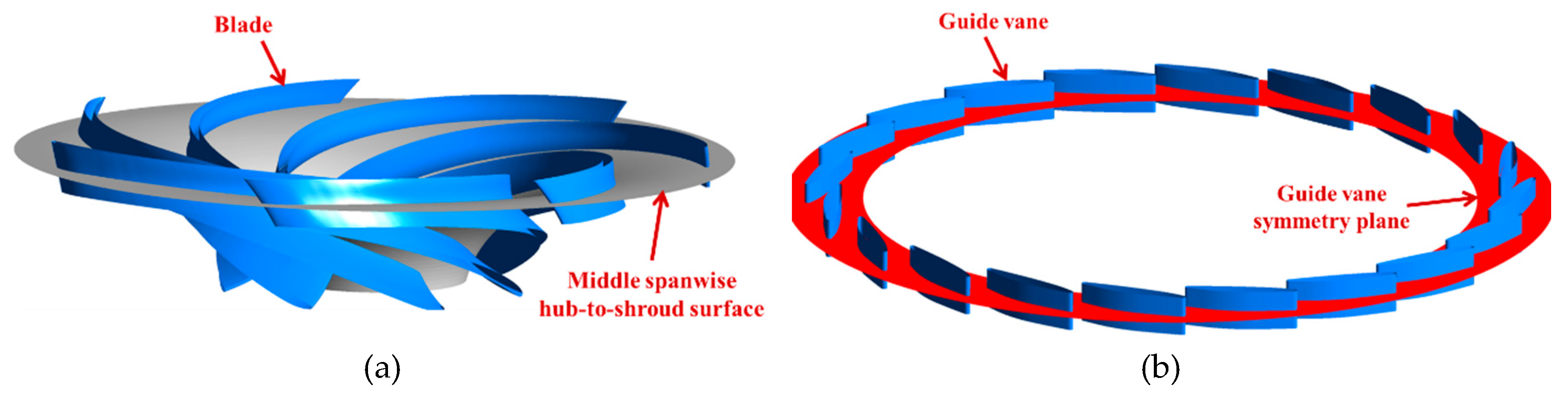
| Number of blades | 7 |
| Impeller inlet diameter (mm) | 250 |
| Impeller outlet diameter (mm) | 550 |
| Number of guide vanes | 20 |
| Height of guide vanes (mm) | 37.75 |
| Number of Grids | ηh (%) | ψ | |
|---|---|---|---|
| Grid system 1 | 8,000,000 | 86.5 | 1.08 |
| Grid system 2 | 12,000,000 | 91.1 | 1.17 |
| Grid system 3 | 17,000,000 | 91.3 | 1.17 |
| Couple of Monitoring Points | vl1-vl2 | vl2-vl3 | vl3-vl4 | vl4-vl1 |
|---|---|---|---|---|
| Cross-phase delay of 1.65 Hz | 272.8 | 260.8 | 304.6 | 241.8 |
© 2019 by the authors. Licensee MDPI, Basel, Switzerland. This article is an open access article distributed under the terms and conditions of the Creative Commons Attribution (CC BY) license (http://creativecommons.org/licenses/by/4.0/).
Share and Cite
Lu, G.; Zuo, Z.; Liu, D.; Liu, S. Energy Balance and Local Unsteady Loss Analysis of Flows in a Low Specific Speed Model Pump-Turbine in the Positive Slope Region on the Pump Performance Curve. Energies 2019, 12, 1829. https://doi.org/10.3390/en12101829
Lu G, Zuo Z, Liu D, Liu S. Energy Balance and Local Unsteady Loss Analysis of Flows in a Low Specific Speed Model Pump-Turbine in the Positive Slope Region on the Pump Performance Curve. Energies. 2019; 12(10):1829. https://doi.org/10.3390/en12101829
Chicago/Turabian StyleLu, Guocheng, Zhigang Zuo, Demin Liu, and Shuhong Liu. 2019. "Energy Balance and Local Unsteady Loss Analysis of Flows in a Low Specific Speed Model Pump-Turbine in the Positive Slope Region on the Pump Performance Curve" Energies 12, no. 10: 1829. https://doi.org/10.3390/en12101829
APA StyleLu, G., Zuo, Z., Liu, D., & Liu, S. (2019). Energy Balance and Local Unsteady Loss Analysis of Flows in a Low Specific Speed Model Pump-Turbine in the Positive Slope Region on the Pump Performance Curve. Energies, 12(10), 1829. https://doi.org/10.3390/en12101829