Abstract
Photovoltaic (PV) and wind power (WT) resources can influence each other in some scenarios, and this influence tends to show that the rise of PV resources may indicate the drop of WT resources, and vice versa. This pattern of PV and WT resources influencing each other is called the complementary characteristics of PV and WT power. The complementary characteristics of the power outputs of different kinds of distributed renewable energy resources (DRERs) and the correlation between DRERs outputs and loads can impact the consumption of DRERs by the loads within the grid, which represents the rate of DRER outputs consumed by loads instead of being reduced. In this regard, this paper investigates a planning strategy for DRERs considering these two factors. An improved co-variance matrix method is applied to generate complementary samples of DRERs and correlated samples of DRERs and loads. The samples generated are used to study the impacts of the degree of correlation between DRERs and loads on the consumption ability of DRERs. The concept of the cluster is introduced as a region including DRERs with complementary characteristics. Based on the cluster partition method and the samples generated, the DRERs planning model is proposed to maximize the profits of different DRER stakeholders. The planning model is transformed into a single objective model through the ideal point method. A Benders decomposition-based method is developed to efficiently solve the proposed model, and an actual network in China is used to illustrate its performance. The results show DRER consumption can be significantly improved by the proposed planning model.
1. Introduction
With the promotion of renewable energy policies in China, more and more distributed renewable energy resources (DRERs) are being connected to power systems. This has led to occurrences of reverse power flows in distribution networks, where energy flows between substations with the same voltage level or from low-voltage substations to an upstream substation. Excessive reverse power flows are usually not allowed in traditional planning strategies of DRERs because they can deteriorate the power quality and result in increased power losses, even breakdown of conventional transformers. Therefore, DRER outputs are reduced or large capacity storage devices are installed to avoid the occurrence of reverse power flows [1]. Recently, some transformers that allow reverse currents have been considered to improve the penetration rate of DRERs [2]. Therefore, it is also possible to limit reverse power flows within a specific region, which includes several substations to increase the overall outputs of DRERs. In this work, the region in the distribution network where reverse power flows are allowed is called a cluster and the process to determine the region is called cluster partitioning.
The consumption of DRERs is affected by two factors: (1) the complementary characteristics of photovoltaic (PV) generation and wind turbine (WT) generation; and (2) the matching characteristics between the power generation and loads. In order to study how these two factors affect the consumption of DRERs, the generation of the data that can represents the complementary characteristics of PV and WT generation and the matching characteristics between power generation and loads using the expected correlation coefficient are essential. The generated two sets of data that are correlated with each other and show the correlation relationship described using correlation coefficients is called correlated samples.
However, there are two obstacles to describe the correlation relationships among PV, WT and load power. One of the difficulties is that the outputs of PVs and WTs are commonly assumed to obey fixed probability distribution functions respectively, which leads to incorrect correlated samples generated by the traditional methods [3,4,5]. The other problem is that it is difficult to choose the suitable parameters to describe the output characteristics of PV and WT generations. The reason for the difficulty of choosing the suitable parameters is that there are no rules to follow of picking the most suitable parameters for the hypothetical distribution functions, and that the hypothetical parameters may not apply to the partial historical data of PV and WT generations due to the randomness of wind speed and solar radiation. Many researchers have discussed the generation of correlated samples. In [3], a traditional correlation coefficient matrix is used to generate the correlated wind speed. This work assumes the wind speed is complied with the normal distribution function, which results in a large forecast error in wind power outputs. A correlated model is established combining the correlation coefficients with the time series in [4], but the assumption remains that the DRERs follow the given probability distribution functions. In [5], a transformation method for the correlated wind speed non-normal distributed based on the Cholesky decomposition is proposed. However, the accuracy of the proposed method is not guaranteed if the distribution functions of WT generation are unknown. Furthermore, the correlated coefficient would be changed during the transformation process. In order to generate the correlated samples satisfying unknown distributed function with expected correlation coefficient, a method of sample generation is proposed in this paper. The proposed method is based on the orthogonal transformation and marginal transformation proposed in [5] as well as the kernel density estimation method in [6], which is an efficient way to directly establish the distribution functions from characteristics of historical data [7].
Many researchers have also addressed the DRER planning problem in recent years. The main goal is to determine the optimal location, capacity, and type of DRERs. The objective function of [8,9] aims to minimize the total network cost. The objective function of [10] aims to minimize distributed generation (DG) installation cost and network losses. In [11], a DG planning scheme is proposed to minimize the network upgrade cost, network loss cost, power interruption cost, and users’ power supply cost. A compromised scheme is obtained in the non-inferior solutions. In [12], a planning model considering the profits of both DG owners and distribution companies are established. The investments and operational costs of DGs as well as the power purchase and interruption costs of distribution companies are minimized in the planning model, and the incomes of DG owners are maximized. This model is established from the view of economy without considering the optimal power losses and voltage profile during the power delivery. In [13], several planning models of DG placement are introduced considering the objectives of the minimum costs and the maximum benefits and loadability with constraints of power flow and power quality. It’s pointed out in [13] that the active network management is essential for the access of high penetration of DG, which involves the reactive and active power control of DGs. According to the above analysis, the previous planning models are usually proposed from the perspectives of economy and optimal power flows. Some aspects are not considered in the previous studies. Firstly, the complementary characteristics of PV generation and WT generation as well as its impact on the planning results are seldom considered in the previous works. Secondly, the previous planning models are built based on one substation and its low voltage networks, therefore the DG installation capacity in such networks cannot excess its maximum load demands. In fact, reverse currents are allowed in some transformers, therefore, the proper power interaction between different substations and the output characteristics of different kinds of DGs should be considered in the planning model. This factor is considered in this paper, along with the complementarity in power supply among substations. To ensure the maximum consumption of DRERs, a planning model is proposed in this paper not only from the perspectives of economy and optimal power flow which are commonly considered in the previous works, but also with the consideration of active power and reactive power control of DRERs based on the actual output characteristics of DRERs and the power interactions between substations.
The planning strategy for DRERs in distribution power systems is usually a non-convex complex optimization problem due to the power flow equations. Intelligent algorithms are widely applied to solve the distribution system planning problem, such as the improved particle swarm optimization [14], genetic algorithm [15], ant colony algorithm [16], and Tabu search method [17]. The drawbacks of these algorithms include a local optimal solution and long computation times. To make the problem tractable, some researchers reformulated the original non-convex model into a convex model based on second-order cone programming (SOCP) [18]. Reference [19] shows the SOCP model is strictly accurate when the objective function is convex and increases with the branch current. To improve the computational efficiency, the complex DRER planning strategy is modeled based on SOCP and decomposed by the Benders decomposition method [20,21].
The planning model is formulated in this paper to maximize the profits of different stakeholders and the consumption ability of the DRERs. To deal with the programming problem with several objectives, some researchers combine Pareto’s multi-objective optimization with modern intelligent algorithms, such as the particle swarm optimization algorithm [22], improved genetic algorithm [23], and evolutionary algorithm [24]. However, this method usually results in a high computational burden to obtain the Pareto solutions. Other researchers established an addable objective by unifying the dimensions of different objectives [25]. The ideal point method, which is applied in this work, can unify the dimensions of different objectives and does not increase the complexity of the original planning problem [26].
A DRER planning model is proposed in this work to improve the consumption ability of the DRERs in a large-scale distribution network, taking the complementarity between the DRERs and correlation characteristics between DRERs and loads into account. First, a sample generation method for correlated WTs, PVs, and loads that follow arbitrary distribution functions is proposed. Then, a planning model for the DRERs based on the clusters is established. The objective function of the planning model is established by through the application of the ideal point method. Benders decomposition is introduced to efficiently solve the proposed model. Finally, an actual distribution system demonstrates the effectiveness of the proposed approach. The contributions of the paper are as follows:
- (1)
- A correlated sample generation method is proposed to generate correlated PV, WT, and load samples following any probability distribution functions. The proposed method can guarantee that the generated samples satisfy the expected correlation coefficient.
- (2)
- The concept of a cluster is introduced to confine the reverse power flows within a region by utilizing the complementary characteristics of PVs and WTs to improve DRER consumption.
- (3)
- A planning model for DRERs is proposed taking the power interaction between different substations within clusters and the complementary characteristics of different kinds of DRERs into consideration. The proposed planning model can improve DRER consumption within clusters.
The remainder of this paper is organized as follows. The generation of correlated WT, PV, and load samples is presented in Section 2. The DRER planning model based on the cluster partition is shown in Section 3. The Benders decomposition model is presented in Section 4. The simulation results are presented in Section 5. Section 6 concludes the paper.
3. DRER Planning Model Based on Cluster Partitioning
3.1. Cluster Partitioning
A cluster in this paper is defined as a set of substations and related lines that form a region within the distribution network. To deal with reverse power flow due to highly penetrated DRERs, this paper divides the distribution network into several clusters, and allows reverse power flow among the substations within a cluster. The clusters are set as the planning units of DRERs within which the complementary outputs of different type of DRERs are used to improve the consumption of hourly outputs. It should be pointed out that the reverse power flows tend to occur simultaneously when all of the substations within a cluster are installed with the same kind of DRERs. In this case, renewable energy consumption in the cluster cannot greatly be improved with the same kind of DRERs within clusters. However, different kinds of DRERs with complementary characteristics installed within a cluster can be utilized to prevent the reverse power of different transformer stations from existing simultaneously. In this way, the matching characteristics between the DRER outputs and the loads within a cluster can be improved.
The above considerations mean that the electrical distance of the nodes included in a cluster should be limited to a relatively suitable range to realize the power interaction. The cluster partition index is used to guarantee the cluster partition results meet the expected standards. Therefore, the cluster partition index proposed in [29], which represents the electrical distance within a cluster, is used in this work. Moreover, the consumption ability of the DRERs installed within a cluster is expected to reach a maximum, which is represented by the index of power balance within each cluster. Therefore, the cluster partition index A is shown as in (5),
where
represents the cluster performance index; represents the index represents the electrical distances between all the nodes within the clusters; represents the index represents the average power balance within all the clusters; represents the set of nodes within the system represents the weight coefficient between node i and j which can be calculated using the (6); Lij represents the electrical distance between node i and j determined by the feeder length; max(L) represents the maximum value of all the Lij; represents the weight of node i which can be calculated using (7); represent set of upstream nodes and downstream nodes of node i, respectively; represents the total weight of all nodes; represents the apparent power of the DRERs within cluster c at time t; represents the apparent power of the loads within cluster c at time t; is 1 if nodes i and j are in the same cluster and 0 otherwise. The power balance in each cluster is the ratio of DRER generation to the total load within the cluster. The Tabu search method proposed in [29] is introduced to solve the cluster partition. The proposed planning model for the DRERs is based on the results of the cluster partition.
In order to deal with the reverse power flow of each substation, this paper divides the distribution networks into clusters, and allows the 35 kV stations within cluster to have reverse power flow which would flow to recent substations with higher load power. However, this reverse power flow will offset the load power of other substations, and the renewable energy access capacity of the cluster still cannot increase greatly. Nevertheless, this problem can be solved if different power plants within the cluster are connected to different kinds of renewable energy with complementary characteristics.
In order to illustrate the necessity and benefit of cluster partition, the schematic diagram of a cluster is shown in Figure 1, consisting of four 35 kV transformer stations (TS) and their networks. The total load profile of the TS 1 and TS 2 are shown as Figure 2a, and the total load profile of the TS 3 and TS 4 are shown as Figure 2b. TS 1 and TS 2 are both installed with high-penetrated distributed PVs, and their load power and PV output curve are shown in Figure 2a. TS 3 and TS 4 are installed with high-penetrated distributed WTs, and their load and WT output curve are shown in Figure 2b. The PV and WT outputs are complementary with each other. The reverse power flow of TS 1 and TS 2 would occur from 9 o’clock to 15 o’clock at noon, and it would flow into TS 3 and TS 4. During the period that the reverse power due to PV outputs flows into TS 3 and TS 4, the WT power outputs of TS 3 and TS 4 is low and these two transformer stations still are able to consume the reverse flow. Therefore, reverse power can be consumed by the load of this cluster with the complementary outputs of PV and WT and can improve the PV planning capacities of the TS 1 and TS 2. As for excessive WT power, the reverse power exists at night or during the period that PV outputs are low and can also supply power to the load of TS 1–4 without affect the consumption of PVs. In summary, the use of complementary characteristics between different DRERs within the cluster can improve the ability of local renewable energy consumption, but the above-mentioned reverse power should not be able to flow in a wide range of networks, otherwise it is prone to appear problems like more network loss and over-voltage, so it is necessary to limit the region of reverse flow according to the result of cluster partition.
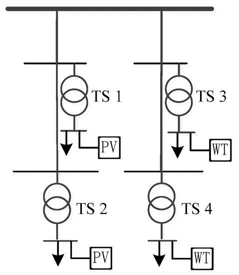
Figure 1.
Simulation figure of substations within a cluster.
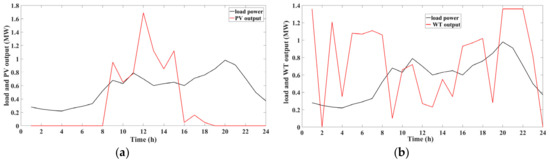
Figure 2.
Relationships between resources and load. (a) Relationships between load and photovoltaic power of TS 1 and TS 2. (b) Relationships between load and wind power of TS 3 and TS 4.
3.2. Planning Model for the DRERs
3.2.1. Objective Function
The objective functions are proposed from both the perspectives of DRER generators and grid operators. As for DRER generators, the investments are expected to reach the minimum, which is shown as (8). Apart from that, the earnings gained from selling energy to grids and governmental subsidies are expected to be as high as possible. This objective is shown as (9), which minimizes the earning loss due to the power reduction through DRER control. The power reduction is expressed by the calculation of the expected DRER outputs minus the actual outputs of DRERs. As for the grid operators, it is expected the accessed DRER can be ultimately consumed by the loads of clusters to improve the power self-supply ability of clusters. This raises the claim to the power match between DRER outputs and loads, and the less hourly power flowed into clusters the better the power match of clusters, which is shown as the objective function (10). It is also an important goal for grid operator to reduce power losses with the access of DRERs, and this objective is shown as (11).
where represent the investment cost and operation cost of photovoltaics (PVs) per MW, respectively; represent the capacity of the PVs and WTs at node i; represent the investment cost and operation cost of wind turbines (WTs) per MW; m represents the number of years in the planning horizon; represents the number of candidate substations for the DRERs; represents the bank rate.
where represents the electricity selling price; represents the governmental subsidies for the DRERs; represents the planning horizon; represent the actual active power outputs of the PVs and WTs at node i at time t, respectively; represent the ratio of the actual active power outputs of the PVs and WTs at node i at time t to their rated power outputs, respectively;
where represents the number of clusters; represents the power flowing into cluster c at time t;
where represents the resistance and reactance of line li-j between nodes i and j; represents the square of current flowing from node i to node j at time t;
The first objective function F1 minimizes the annual investments and operation costs of the DRERs and F2 is the benefit losses due to the reduction of DRER outputs. Both F1 and F2 represent revenue brought by the DRERs. The third objective function F3 minimizes the electricity energy flowing into clusters and the fourth objective function F4 minimizes power losses within the clusters.
The dimensions of the four objectives are different. Therefore, it is unreasonable to directly add them together to form the single objective function. The ideal point method is utilized to transform these objective function values into the deviation values from their ideal values. The ideal values of the four objectives are assumed as , , , and , respectively. The actual values of four objectives are assumed to be bigger or smaller than the ideal values of objectives. The deviation is introduced into the transformed objective function. Therefore, the four objective functions are transformed into the single objective function as shown in (12) using the to represent the deviation distance between the actual value and idea value of the th objective function. Due to the dimension difference, the in (12) is used to normalize the deviation distance of different deviation distances.
where is the positive and negative deviations between the actual value and ideal value in the th objective function, respectively; , are the objective function and weight coefficient representing its priority, respectively.
3.2.2. Constraints
(1) Constraints on Deviations
The deviation variables in (12) should satisfy the equality constraints shown in (14)–(18):
(2) AC Power Flow Constraints
Based on the branch power flow, the AC power flow constraints are relaxed and formulated as per the SOCP model:
where represent the active and reactive power flow from node i to node j at time t, respectively; represents the reactance of line li-j between nodes i and j; , represent the active and reactive power of loads at node i at time t, respectively; , represent the Reactive power outputs of the PVs and WTs at node i at time t, respectively; represents the square of the voltage at node i at time t; and represent the upper and lower limits of the nodal voltages, respectively; represents the maximum value of current; (19) and (20) are the active and reactive power balance constraints; (21) represents the voltage relationships between nodes at two terminals of a connected branch; (22) represents the relaxed branch current expression within the network; (23) represents the minimum and maximum constraints of the nodal voltages; and (24) represents the minimum and maximum constraints of the line currents.
(3) Constraints on the penetration rate of clusters
The installed DRER capacities should be limited within a specified threshold. In this paper, the concept of penetration rate is introduced to limit the overall capacities of the DRERs within a cluster. The definition of the penetration rate of a cluster is shown in (25):
where represents the apparent power of substation i; represents the penetration rate of DRERs within a cluster;
The penetration rate of any cluster c is constrained to excess a specified value. The constraint is as shown in (26):
where represents the expected value of of the penetration rate of DRERs within a cluster
(4) Constraints on the active power outputs of the DRERs
(5) Constraints on the reactive power outputs of DRERs
Two kinds of DRERs are installed at each substation. One kind of DRER does not participate in voltage regulation and the reactive power outputs are limited by their power factors. The other kind of DRER is involved in voltage regulation, with their reactive power outputs limited by their rated capacities. The power factor of the DRER is set as 0.95 based on the operational standard of grid in China.
Constraints of the reactive power of DRERs that do not participate in the voltage regulation are shown as
Constraints of the reactive power of DRERs that participate in the voltage regulation are (31) and (32).
4. Establishment and Calculation of the Benders Decomposition Model
The bulleted lists appear as follows: To improve the computational efficiency, the proposed planning model is decomposed into a master problem (MP) and a sub-problem (SP). The master problem is an investment problem, whose decision variables are the installation capacities and the types of DRERs. The sub-problem deals with the optimal power flow problem, and the decision variables include the actual active and reactive power outputs of the DRERs, nodal voltages, currents, and transmission power of each line. The standard form of the proposed planning model is as follows:
where represents the coefficient matrix of objective function correlated with investment problem; represents the variables of the installation capacities and the types of DRERs; represents the coefficient matrix of objective function correlated with optimal power flow problem; represents the variables including the actual active and reactive power outputs of the DRERs, nodal voltages, currents, and transmission power of each line; represents the coefficient matrix correlated with variables of penetration rate of clusters of equality constraints; represents the matrix of expected penetration rate of clusters of equality constraints; represents the coefficient matrix correlated with variables of the installation capacities and the types of DRERs of inequality constraint ; represents the coefficient matrix correlated with variables of actual active and power outputs of the DRERs of inequality constraint ; represents the constant of inequality constraint ; represents the coefficient matrix correlated with variables of actual active and reactive power outputs of the DRERs, nodal voltages, currents, and transmission power of each line of second-order-cone constraint ; represents the coefficient matrix correlated with variables of nodal voltages and currents of second-order-cone constraint ; represents the coefficient matrix correlated with variables of the installation capacities of second-order-cone constraint ; represents the coefficient matrix correlated with variables of actual active and power outputs of the DRERs, nodal voltages, and currents of inequality constraint ; represents the constraint of nodal voltage, current, and actual active and reactive power output of DRER of inequality constraint ; represents the coefficient matrix correlated with variables of actual active and power outputs of the DRERs, nodal voltages, positive deviation and negative deviation of objective functions of equality constraint ; represents the constant including active, reactive load power and ideal value of objective function of equality constant ; (37) represents (26)–(28); (38) represents (29) and (30); (39) represents (22), (33) and (34); (40) represents (23), (24), (31) and (32); and (41) represents (14)–(17) and (19)–(21).
The MP is formulated as:
The SP is presented as:
The dual form of the SP is expressed as:
The steps for solving the Benders decomposition-based model are as follows.
Step 1: Solve the MP and obtain the lower bound of the original problem (36)–(42) and the decision variable .
Step 2: Solve the SP and check whether it is feasible.
(a) If the SP is infeasible, introduce the relax variables and formulate the relaxed SP (57)–(61), called the RSP. Go to step 3.
where represents the relax variable of corresponding with constraint of type .
(b) If the SP is feasible, calculate the upper bound . Check whether is satisfied. If so, stop the iteration and output the results. Otherwise, generate the feasibility cut (62), and add it into the MP, then return to Step 1.
Step 3: Solve the RSP, and add the infeasibility cut (63) into the MP, then return to Step 1.
The calculation process of the proposed method is shown in Figure 3.
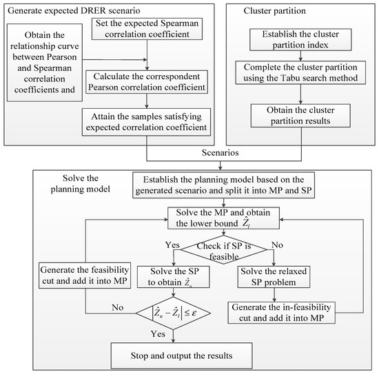
Figure 3.
Calculation process of the proposed method.
5. Case Study
An actual distribution network is applied in this paper to illustrate the efficiency of the proposed model. The network consists of 31 candidate substations. The numerical results are obtained using a laptop computer with a 3.3 GHz Intel Core i5-4590 CPU and 8 GB of memory.
5.1. Expected Correlated Samples of the PVs and WTs
According to the Section 2.1 and Section 2.2, in order to apply the proposed method of generating the expected PV and WT samples into the actual distribution system in China, it is necessary to calculate cumulative probability functions of PV and WT according to the historical data based on the kernel density estimation. The results of cumulative probability functions at different time of the day are shown as Figure 4 and Figure 5.
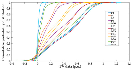
Figure 4.
Cumulative probability functions of PV data during the times of t=6-18.
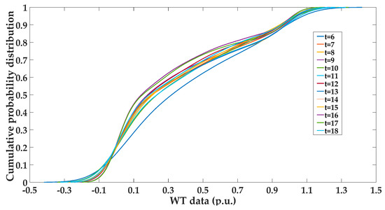
Figure 5.
Cumulative probability functions of WT data during the times of t=6-18.
Based on the results shown in Figure 4 and Figure 5, the relationships between the Pearson correlation coefficients used to describe the standard normal distributed variables and the Spearman correlation coefficients used to describe the PV and WT data can be obtained through the steps 1–6. The results of the relationships at two different time periods of the day are shown as Figure 6. It can be seen that the differences of the relationships of correlation coefficients under different time periods of the day are trivial. The expected PV and WT samples can be obtained using the data shown in Figure 6 through Steps 7 and 8 of Section 2.2.
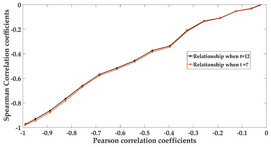
Figure 6.
Relationships between Pearson correlation coefficient and Spearman correlation coefficient.
To illustrate the effectiveness of the proposed correlated sample generation method, the comparison of correlation coefficients of generated samples attained by two methods is made. Two cases are defined as follows.
Case 1: Assume that the PV and WT outputs satisfy the Beta and Weibull distribution respectively. The correlated samples of PV and WT outputs are generated using the orthogonal transformation in [5].
Case 2: Correlated samples of PV and WT outputs are generated by the proposed method in this paper.
The expected PV and WT samples with different complementary characteristics are shown as Figure 7, and the results of these two cases under different correlation coefficients are close to each other. It’s seen from Table 1 that the correlation coefficients of samples in Case 2 are closer to the expected correlation coefficients than those in Case 1. Therefore, the effectiveness and the accuracy of the proposed method for generating correlated samples can be verified.
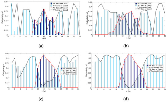
Figure 7.
Generated complementary PV and WT of Cases 1 and 2 under different correlation coefficients. (a) η = −0.2; (b) η = −0.5; (c)η = −0.8; (d) η = −1.

Table 1.
Correlated samples in Case 1 and Case 2.
The correlated hourly PV and WT samples in a day are shown in Figure 8, where the increase in absolute value of the negative correlation coefficient between the PV and WT outputs represents the rise in complementary characteristics between the PV and WT outputs.
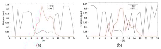
Figure 8.
Samples of correlated PV and WT outputs with expected Spearman correlation coefficients. (a) η = −0.95. (b) η = −0.65.
5.2. Cluster Partition Results
The topology and cluster partition results calculated using the method of Section 3.1 are shown in Figure 9, where the light blue blocks represent the different clusters. The distribution network is divided into 8 clusters based on the cluster partition indexes and method in Section 3.1. There are negative power demands at 11 substations, located at nodes 11, 15, 29, 31, 36, 40, 42, 43, 48, 51, and 52.
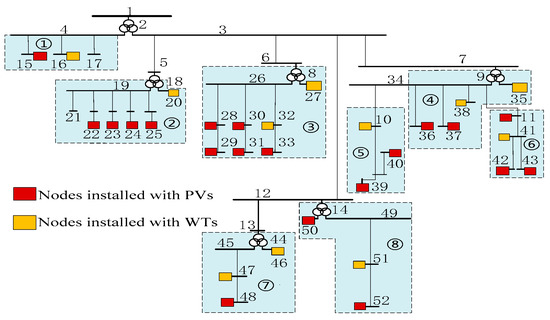
Figure 9.
Topology of an actual network and the results of cluster partition.
The calculated cluster partition indexes are shown as Table 2. The value of index is calculated based on the power balance of clusters which are also shown in the Table 2. The power balance of the clusters represents the consumption of the DRERs original installed within the clusters. The lower the index of the power balance is, there are more PVs/WTs still can be installed into the cluster, and the power balance of cluster 2, 3, 4, 7, 8 is relatively lower, which represents there are more PV and WT can be installed within these five clusters.
Table 2.
The cluster partition indexes.
5.3. Comparison of PV and WT Planning Solutions with/without Cluster Partitioning
The investment costs of the PVs and WTs are assumed to be $1.56 million per MW and $1.09 million per MW based on the data in [30] combined with the practical engineering experiences in China, respectively. The annual operating costs of the PVs and WTs are assumed to be 1% of the annual investment cost. The number of years in the planning horizon is 20 and the interest rate is 4.9%. The Spearman correlation coefficient of the WTs and PVs is −0.85 and the penetration rates of the clusters are 0.8. Two cases are defined as follows.
Case 3: Assume that cluster partition is not considered in the proposed DRER planning model;
Case 4: Assume that cluster partition is considered in the proposed DRER planning model.
The PV and WT planning solutions in Case 3 are obtained by solving the decomposed model proposed in this paper. The computation time is 229.392 s. The decomposed model proposed in this paper converges after three iterations, which verifies the advantages of the proposed model.
To obtain the planning solution without the cluster partitions, the energy flowing into each cluster in the proposed model is replaced by the energy flowing into the entire power system, and the cluster penetration rate is replaced by the penetration rate of the distribution system. Substations that have negative power demands are not allowed to install DRERs and reverse power flows are not allowed in the system.
The capacities of PVs and WTs in the planning solution with/without the cluster partitions are shown in Table 3.
Table 3.
Planning results for Case 3 and Case 4.
It’s shown in Table 4 that PVs can be installed in the substations with negative power demands in Case 4, while no PVs are installed in the substations with negative power demands in Case 3. Furthermore, the installation of WTs increases in Case 4 compared to the results for Case 3, which could lead to fewer investment costs. It’s shown in Table 4 that the investment and operating costs, the power losses of the network, and the energy flow into the system for Case 3 and Case 4. The investment costs in Case 4 are lower by $730,226 compared to Case 3, which indicates that the economic efficiency is enhanced in the planning solution with the cluster partitions. The power losses and energy flow into the system in Case 4 drop by 23.18% and 43.14%, respectively, compared to those in Case 3, which indicates the overall outputs of the DRERs in Case 4 are significantly improved. Therefore, this confirms the proposed planning model taking the cluster partition into account can improve DRER consumption.
Table 4.
Comparison of planning results between Case 3 and Case 4.
The voltage characteristics of the DRERs in Case 3 and Case 4 are shown in Table 5. The voltage fluctuation range in the planning solution in Case 4 increases by 2.74% compared to that in Case 3. The power exchanges between substations increase the voltage volatility. The planning solution in Case 1 will therefore be at the expense of voltage fluctuations.
Table 5.
Voltage characteristics of nodal voltage of different cases.
5.4. Impacts of the Complementary Characteristics on Planning Results
In order to illustrate the impact of different complementary characteristics of PV and WT outputs on the access planning of DRERs, there are four cases as followed being compared and analyzed.
Case 5: Penetration rates in each cluster are 0.80 and the Spearman correlation coefficient of the PV and WT outputs is −0.95;
Case 6: Penetration rates in each cluster are 0.80, and the Spearman correlation coefficient of the PV and WT outputs is −0.65;
Case 7: Penetration rates in each cluster are 0.50, and the Spearman correlation coefficient of the PV and WT outputs is −0.95;
Case 8: Penetration rates in each cluster are 0.50, and the Spearman correlation coefficient of the PV and WT outputs is −0.65.
These four cases are accomplished in the IEEE 33 bus system shown in Figure 10 and the actual networks shown in Figure 9.
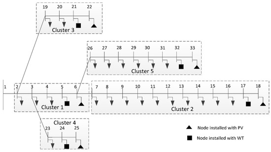
Figure 10.
Topology of IEEE 33 bus system.
The planning capacities of DRERs in each cluster of Cases 5-8 for the IEEE 33 bus system is shown in Table 6. Figure 11 shows the planning capacities of PVs/WTs at each candidate node in the eight clusters. The bars in dark blue represent the substations installed with the PVs, and the bars in light blue represent the substations installed with the WTs. Four consecutive bars are regarded as a group, and represent the optimal capacity results in Case 5, Case 6, Case 7, and Case 8, respectively.
Table 6.
Planning capacities of WT/PV of Cases 5–8 for the IEEE 33 bus system.
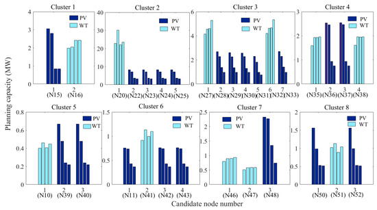
Figure 11.
Comparison of the optimal capacities of the PVs/WTs of substations in each cluster of the actual network.
Table 6 and Figure 11 of two different networks show the capacity ratio of the WTs to all of the DRERs in each cluster increases when the complementary characteristics between the PVs and WTs drop. This is because the installation and operating costs of the WTs are lower than those of the PVs. Moreover, WTs can provide active outputs on all days, which lead to less energy flow into the clusters when the complementary characteristics between the PVs’ and WTs’ drop.
In this work, the reduction rate of the PV and WT outputs shown in Table 7 is defined as the predicted PV and WT outputs divided by their actual outputs. Table 7 shows the reduction rates of the PVs and WTs both decline due to the rise of complementary characteristics between PVs and WTs. It’s seen from the results of IEEE 33 bus system that the PV reduction rate and the WT reduction rate in Case 5 decrease by 7.89% and 9.37% compared to those in Case 6, respectively. The PV reduction rate and the WT reduction rate in Case 7 decrease by 0.33% and 1.31% compared to those in Case 8, respectively. According to the results of the actual network, the PV reduction rate and the WT reduction rate for a penetration rate of 0.80 in Case 5 decrease by 5.15% and 5.75% compared to those in Case 6, respectively. The PV reduction rate and the WT reduction rate for a penetration rate of 0.50 in Case 7 decrease by 0.03% and 0.88%, respectively, compared to those in Case 8. Thus, the drop in WT reduction rate exceeds the drop in PV reduction rate when the complementary characteristics between PVs and WTs rise. The voltage fluctuation range of the IEEE 33 bus system in Case 6 is 3.92% more than that in Case 5. The voltage fluctuation range of the actual network in Case 6 is 2.74% more than that in Case 5. The voltage fluctuation range of the IEEE 33 bus system in Case 8 is 3.37% more than that of Case 7. The voltage fluctuation range of the actual network in Case 8 is 1.50% more than that of Case 7. Therefore, the rise in complementary characteristics between PVs and WTs decreases the voltage fluctuation range. This is because the rise in complementary characteristics between the PVs and WTs reduces the probability that PV and WT outputs simultaneously increase or decrease, and thus results in smaller nodal voltage fluctuation. Table 7 also shows the power losses within clusters rise as the penetration rate increases due to the increase of reverse power flows within clusters. The energy flow into clusters decreases as the penetration rate increases, which leads to the increasing power balance of clusters. If the loads in the clusters are fixed, the decreased energy flowing into clusters exceeds the decreased power losses within clusters when the complementary characteristics between PVs and WTs rise. In this way, the DRER outputs increase with the rise of complementary characteristics between PVs and WTs. Therefore, an increase in complementary characteristics between PVs and WTs within clusters helps improve the consumption abilities of DRERs.
Table 7.
Overall reduction rates in different cases.
5.5. Impacts of the Spearman Correlation Coefficients between the DRERs and Loads on the Planning Results
In order to illustrate the impact of the variation of the correlation relationship between DRERs and loads on DRER access planning results, there are four cases in this subsection are compared and analyzed. In this subsection, the Spearman correlation coefficient between PV and WT outputs is −0.85. The following scenarios are compared and analyzed.
Case 9: Penetration rates of the clusters are 0.85, and the Spearman correlation coefficient between the DRERs and loads is 0.90;
Case 10: Penetration rates of the clusters are 0.85, and the Spearman correlation coefficient between the DRERs and loads is 0.30;
Case 11: Penetration rates of clusters are 0.45, and the Spearman correlation coefficient between the DRERs and loads is 0.90;
Case 12: Penetration rates of clusters are 0.45, and the Spearman correlation coefficient between the DRERs and loads is 0.30.
Table 8 shows that the increase in correlation coefficient between the DRERs and loads results in a decrease in the reduction rate of DRER outputs. As the correlation coefficient between the DRERs and loads increases, the power losses and the energy flow into clusters increase. Comparing the power losses within clusters and energy flow into clusters shows the decreased energy flow into clusters exceeds the decreased power losses within clusters as the correlation coefficient of DRERs and loads increases. This indicates a rise in DRER outputs. Therefore, the increase in the correlation coefficient between the DRERs and loads helps improve the consumption abilities of DRERs.
Table 8.
Comparison of planning results for different cases.
6. Conclusions
In order to study the effects of complementary relationship between WTs and PVs and the matching characteristics between the power generation and loads on the planning and consumption of DRERs, a method is proposed in this paper to generate correlation scenarios of WTs, PVs, and loads based on an improved correlation matrix method, orthogonal transformation and the kernel density estimation method. A planning model of the complementary DRERs in a high-penetrated distribution power system is then established, which aims to maximize the profits of different stakeholders and the DRER consumption ability within clusters. The effectiveness of the Benders decomposition model is demonstrated using an actual distribution system. What’s more, the impacts of the complementary relationship between PV generation and WT generation and the matching characteristics between the power generation and loads on the planning solutions as well as consumption of DRERs are studied in the case study. The case study indicates that
- (1)
- The proposed planning model could improve DRER consumption ability by introducing the cluster concept as well as correlated DRER samples.
- (2)
- The better complementary characteristics of PVs and WTs within clusters could lead to an increase in the ratio of PVs to DRERs planned in the clusters and better DRER consumption ability.
- (3)
- The increase of the correlation coefficient between DRERs and loads helps to reduce the reduction rate of DRER outputs and power losses. Therefore, the consumption abilities of DRERs can be improved.
Author Contributions
D.H. helped design the study, analyse the data, and write the manuscript. M.D. helped conduct the study and edit the manuscript. S.L. and J.Z. helped edit the manuscript.
Funding
This research was funded by [the National Key R&D Program of China] grant number [2016YFB0900400].
Acknowledgments
This work was funded by a project supported by the National Key R&D Program of China (The key technologies and demonstrative application for the integration and consumption of clustered distributed renewable energy generation) (2016YFB0900400).
Conflicts of Interest
The authors declare no conflicts of interest.
References
- Hu, D.; Ding, M.; Bi, R.; Rong, X. Sizing and placement of distributed generation and energy storage for a large-scale distribution network employing cluster partition. J. Renew. Sustain. Energy 2018, 10. [Google Scholar] [CrossRef]
- Cho, G.J.; Kim, C.H.; Oh, Y.S.; Kim, M.S.; Kim, J.S. Planning for the future: Optimization-based distribution planning strategies for integrating ditributed energy resources. IEEE Power Energy Mag. 2018, 16, 77–87. [Google Scholar] [CrossRef]
- Feijóo, A.E.; Cidrás, J.; Dornelas, J.L.G. Wind speed simulation in wind farms for steady-state security assessment of electrical power systems. IEEE Trans. Energy Conver. 1999, 14, 1582–1588. [Google Scholar] [CrossRef]
- Correia, P.F.; Ferreira, J.M. Simulation of correlated wind speed and power variates in wind parks. Elect. Power Syst. Res. 2010, 80, 592–598. [Google Scholar] [CrossRef]
- Morales, J.M.; Baringo, L.; Conejo, A.J.; Mínguez, R. Probabilistic power flow with correlated wind sources. IET Gener. Trans. Distrib. 2010, 4, 641–651. [Google Scholar] [CrossRef]
- Pagan, A.; Ullah, A. Nonparametric Econometrics; Cambridge University Press: London, UK, 1999. [Google Scholar]
- Sun, G.L.; Lang, F.; Yang, M.; Hua, J. Application protocols identification using non-parametric estimation method. In Proceedings of the 2011 6th International Forum on Strategic Technology, Harbin, Heilongjiang, China, 22–24 August 2011; pp. 765–768. [Google Scholar]
- Hien, N.C.; Mithulananthan, N.; Bansal, R.C. Location and sizing of distributed generation units for loadability enhancement in primary feeder. IEEE Syst. J. 2013, 7, 797–806. [Google Scholar] [CrossRef]
- Yammania, C.; Maheswarapub, S.; Mayam, S. Multiobjective Optimization for optimal placement and size of DG using Shuffled Frog Leaping Algorithm. Energy Procedia 2012, 14, 990–995. [Google Scholar] [CrossRef]
- Celli, G.; Ghiani, E.; Mocci, S.; Pilo, F. A multiobjective evolutionary algorithm for the sizing and siting of distributed generation. IEEE Trans. Power Syst. 2005, 20, 750–757. [Google Scholar] [CrossRef]
- Gao, Y.; Hu, X.; Yang, W.; Liang, H.; Li, P. Multi-objective bilevel coordinated planning of distributed generation and distribution network frame based on multiscenario technique considering timing characteristics. IEEE Trans. Sustain. Energy 2017, 8, 1415–1429. [Google Scholar] [CrossRef]
- Ameli, A.; Bahrami, S.; Khazaeli, F.; Haghifam, M.-R. A Multiobjective Particle Swarm Optimization for Sizing and Placement of DGs from DG Owner’s and Distribution Company’s Viewpoints. IEEE Trans. Power Deliv. 2014, 29, 1831–1840. [Google Scholar] [CrossRef]
- Georgilakis, P.S.; Hatziargyriou, N.D. Optimal distributed Generation Placement in Power Distribution Networks: Models, Methods, and Future Research. IEEE Trans. Power Syst. 2013, 28, 3420–3428. [Google Scholar] [CrossRef]
- Soroudi, A.; Afrasiab, M. Binary PSO-based dynamic multi-objective model for distributed generation planning under uncertainty. IET Ren. Power Gener. 2012, 6, 67–78. [Google Scholar] [CrossRef]
- Ganguly, S.; Samajpati, D. Distributed generation allocation on radial distribution networks under uncertainties of load and generation using genetic algorithm. IEEE Trans. Sustain. Energy 2015, 6, 688–697. [Google Scholar] [CrossRef]
- Tolabi, H.B.; Ali, M.H.; Rizwan, M. Simultaneous reconfiguration, optimal placement of DSTATCOM, and photovoltaic array in a distribution system based on Fuzzy-ACO approach. IEEE Trans. Sustain. Energy 2014, 6, 210–218. [Google Scholar] [CrossRef]
- Katsigiannis, Y.A.; Georgilakis, P.S.; Karapidakis, E.S. Hybrid simulated annealing–Tabu search method for optimal sizing of autonomous power systems with renewables. IEEE Trans. Sustain. Energy 2012, 3, 330–338. [Google Scholar] [CrossRef]
- Farivar, M.; Low, S.H. Branch flow model: Relaxations and convexification part I. IEEE Trans. Power Syst. 2013, 28, 2554–2564. [Google Scholar] [CrossRef]
- Low, S.H. Convex relaxation of optimal power flow-part II: Exactness. IEEE Trans. Contr. Net. Syst. 2014, 1, 177–189. [Google Scholar] [CrossRef]
- Khodaei, A.; Bahramirad, S.; Shahidehpour, M. Microgrid planning under uncertainty. IEEE Trans. Power Syst. 2014, 30, 2417–2425. [Google Scholar] [CrossRef]
- Nasrolahpour, E.; Kazempour, S.J.; Zareipour, H.; Rosehart, W.D. Strategic sizing of energy storage facilities in electricity markets. IEEE Trans. Sustain. Energy 2016, 7, 1462–1472. [Google Scholar] [CrossRef]
- Huang, Y.C. Enhanced genetic algorithm-based fuzzy multi-objective approach to distribution network reconfiguration. IET Gener. Transm. Distrib. 2002, 149, 615–620. [Google Scholar] [CrossRef]
- He, Z.; Yen, G.G.; Yi, Z. Robust multi-objective optimization via Evolutionary Algorithms. IEEE Trans. Evol. Comp. 2018. [Google Scholar] [CrossRef]
- Xu, Z.S.; Liu, H.F. A practical method of multiobjectives optimum decision. Oper. Resear. Manag. Sci. 2000, 9, 74–78. [Google Scholar]
- Andervazh, M.; Olamaei, J.; Haghifam, M. Adaptive multi-objective distribution network reconfiguration using multi-objective discrete particles swarm optimisation algorithm and graph theory. IET Gener. Transm. Distrib. 2013, 7, 1367–1382. [Google Scholar] [CrossRef]
- Hu, F.; Geng, Z.; Chen, H.; Sun, L. Research of multi-resource and multi-objective emergency scheduling based on fuzzy ideal point Method. In Proceedings of the 2018 International Conference on Computational Intelligence and Security, Suzhou, China, 13–17 December 2008; pp. 91–95. [Google Scholar]
- McKinley, S.; Levine, M. Cubic spline interpolation. Available online: http://online.redwoods.cc.ca.us/instruct/darnold/laproj/Fall98/Sky Meg/proj.pdf (accessed on 10 May 2019).
- Kendall, M.; Gibbons, J.D. Rank Correlation Method; Oxford University Press: London, UK, 1990. [Google Scholar]
- Chai, Y.; Guo, L.; Wang, C.; Zhao, C.; Du, F.; Pan, J. Network partition and voltage coordination control for distribution networks with high penetration of distributed PV units. IEEE Trans. Power Syst. 2018, 33, 3396–3407. [Google Scholar] [CrossRef]
- Xu, S.; Li, Y. Optimal allocation of distributed generators in distribution network based on time-sequence characteristics. Modern Electr. Power 2019, 36, 8–16. (In Chinese) [Google Scholar]


© 2019 by the authors. Licensee MDPI, Basel, Switzerland. This article is an open access article distributed under the terms and conditions of the Creative Commons Attribution (CC BY) license (http://creativecommons.org/licenses/by/4.0/).