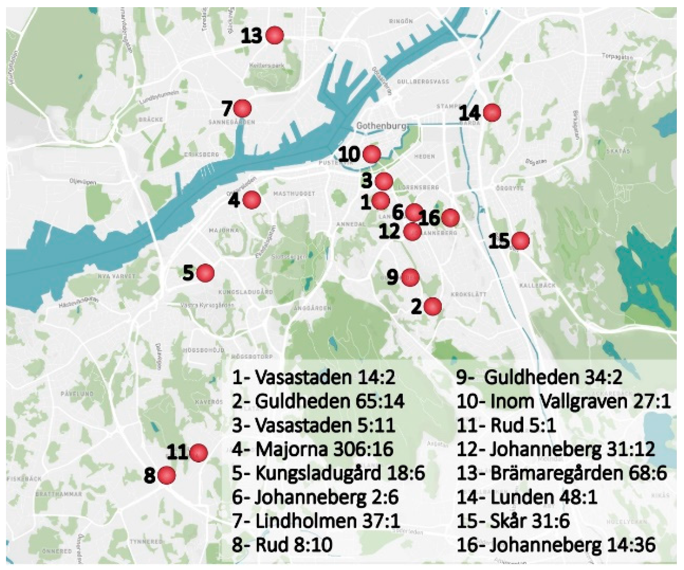
Figure 1.
Location of the studied buildings in Gothenburg. The cadastral numbers are shown next to the ID.
Figure 1.
Location of the studied buildings in Gothenburg. The cadastral numbers are shown next to the ID.
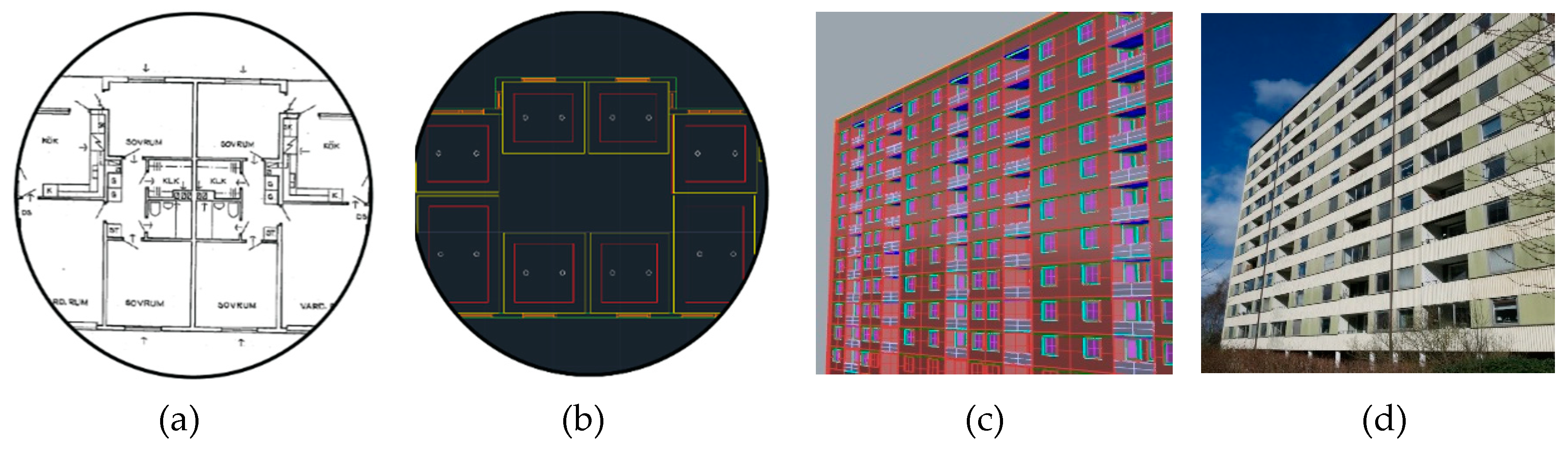
Figure 2.
Creating CAD replicas of a building: (a) the original (scanned) blueprint of a floor plan; (b) the same floor plan redrawn in AutoCAD; (c) a 3D model of the building in Rhino, reconstructed from the floor plans; and (d) a photo of the actual building (ID 2).
Figure 2.
Creating CAD replicas of a building: (a) the original (scanned) blueprint of a floor plan; (b) the same floor plan redrawn in AutoCAD; (c) a 3D model of the building in Rhino, reconstructed from the floor plans; and (d) a photo of the actual building (ID 2).
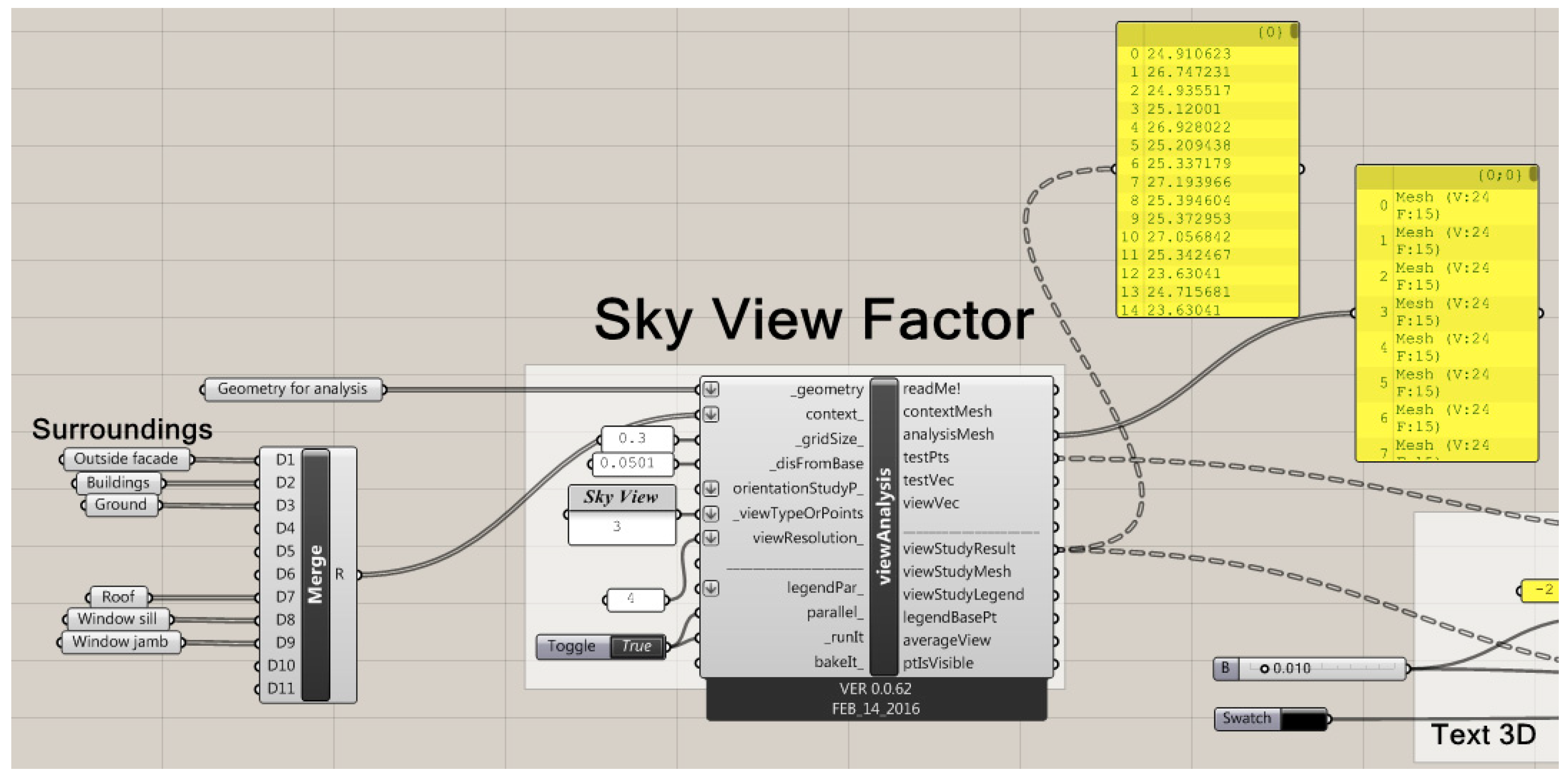
Figure 3.
Calculation of the sky view factor in Grasshopper.
Figure 3.
Calculation of the sky view factor in Grasshopper.
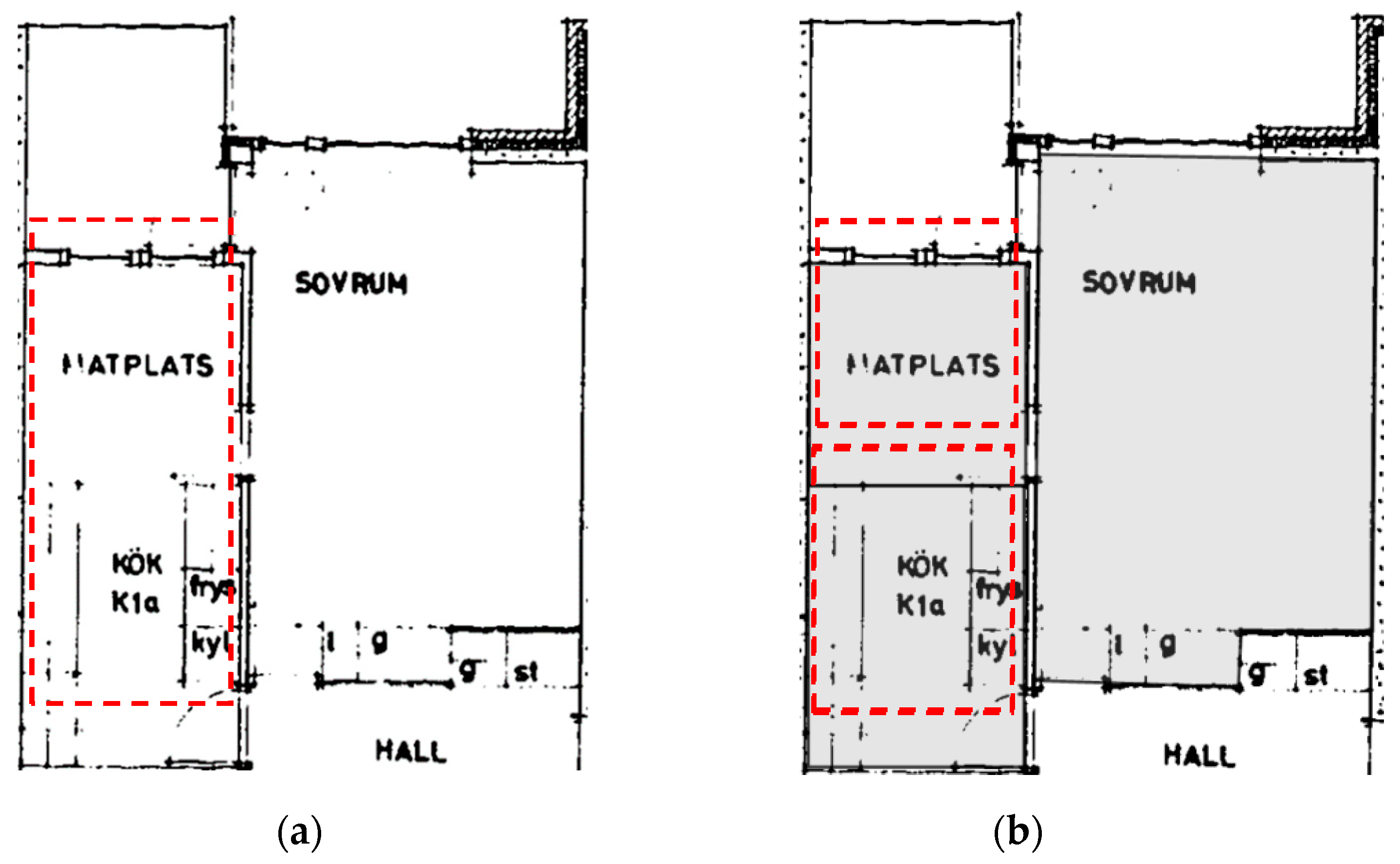
Figure 4.
Separation of an open floor plan into two entities: (a) The original plan with a kitchen and a dining room (within the dashed line) and (b) a wall added between these two rooms for DFP calculations.
Figure 4.
Separation of an open floor plan into two entities: (a) The original plan with a kitchen and a dining room (within the dashed line) and (b) a wall added between these two rooms for DFP calculations.
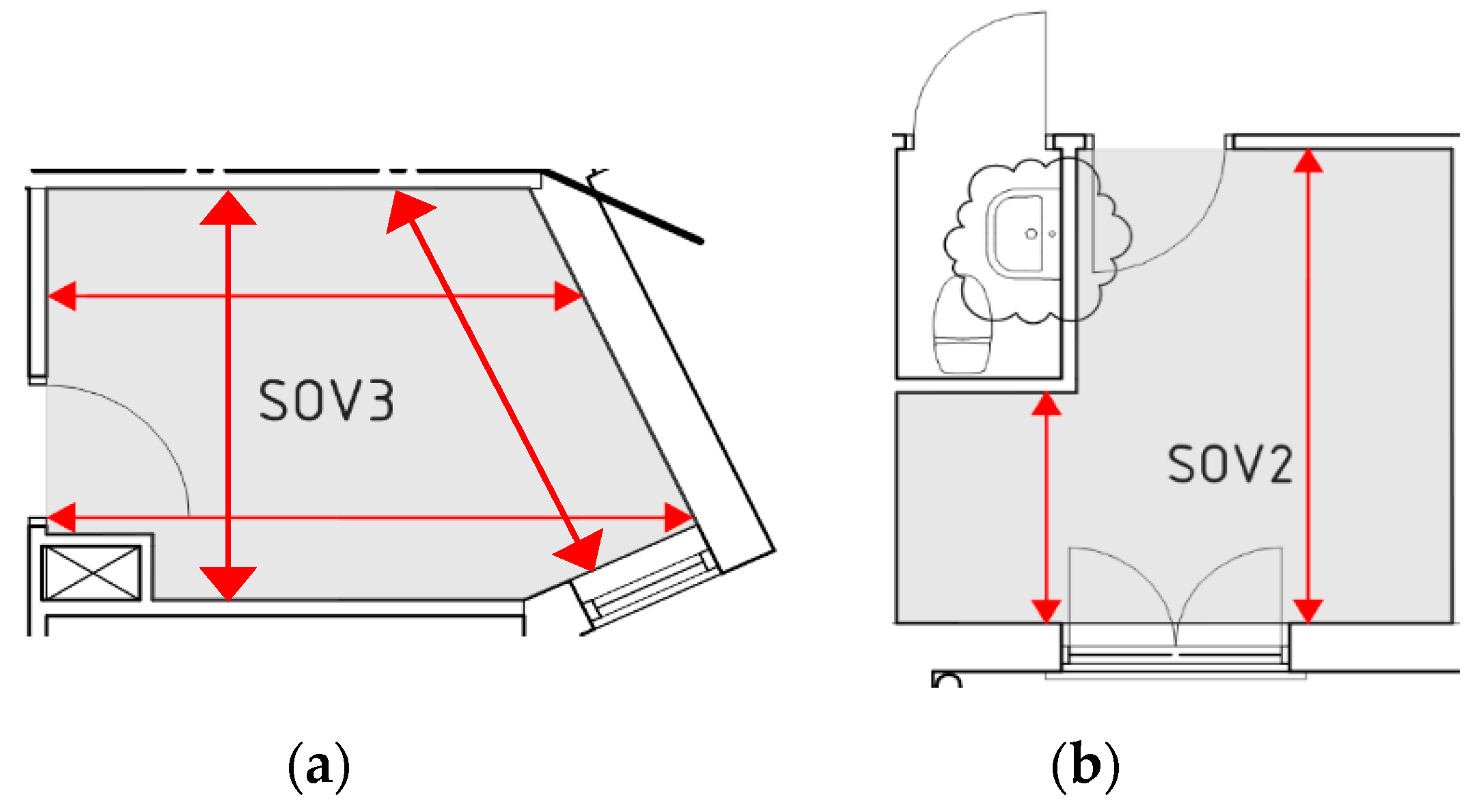
Figure 5.
Rooms with varying room depths in: (a) Different directions and (b) one direction.
Figure 5.
Rooms with varying room depths in: (a) Different directions and (b) one direction.
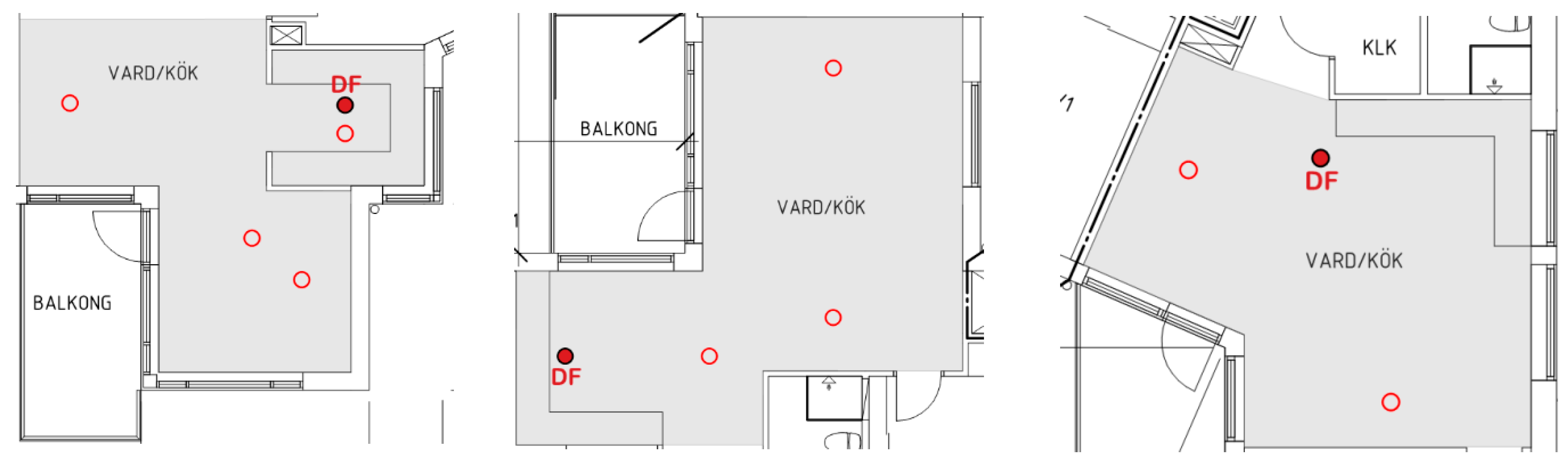
Figure 6.
Examples of combined kitchens and living rooms that result in complex floor layouts. Acceptable positions for the evaluation of single-point DF are indicated with circles. Positions with the lowest calculated single-point DF are shown by dots.
Figure 6.
Examples of combined kitchens and living rooms that result in complex floor layouts. Acceptable positions for the evaluation of single-point DF are indicated with circles. Positions with the lowest calculated single-point DF are shown by dots.
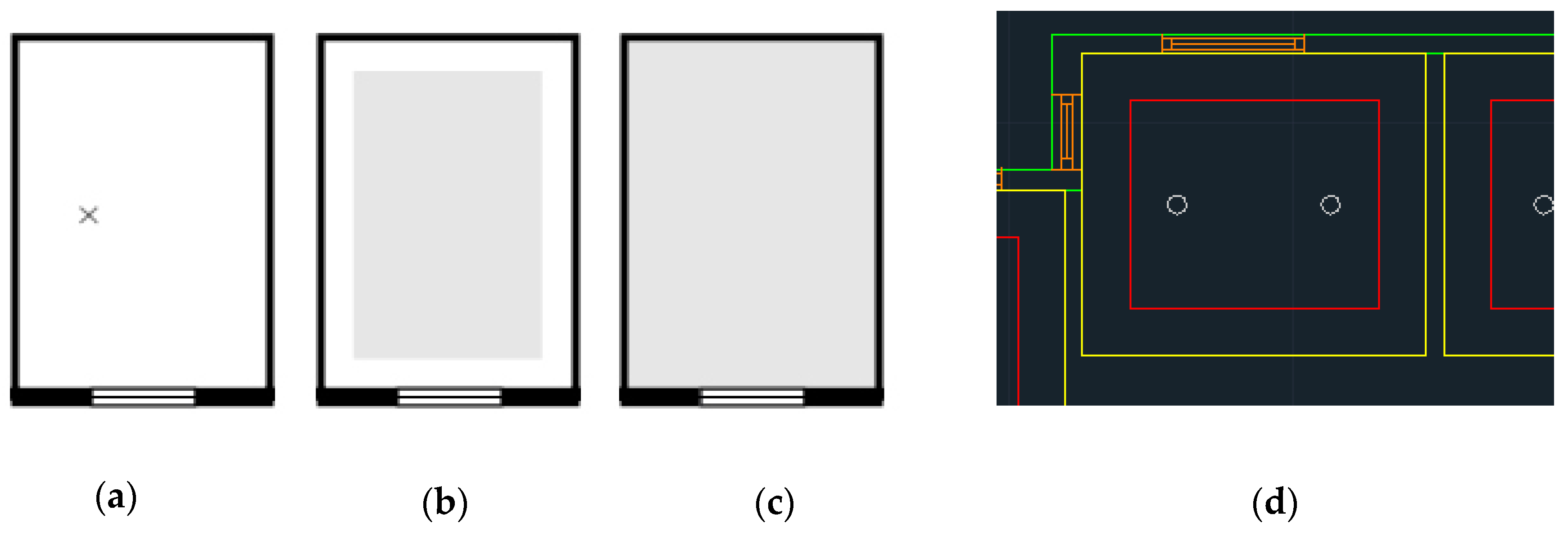
Figure 7.
Control points and control surfaces for DF calculations in a room: (a) The control point for DFP; (b), and the retracted and (c) whole control surface for DFA and DFM. (d) A drawing of a floor plan in AutoCAD with the control points (white circles) and the retracted and the whole control surfaces, enclosed by the red and yellow rectangles, respectively.
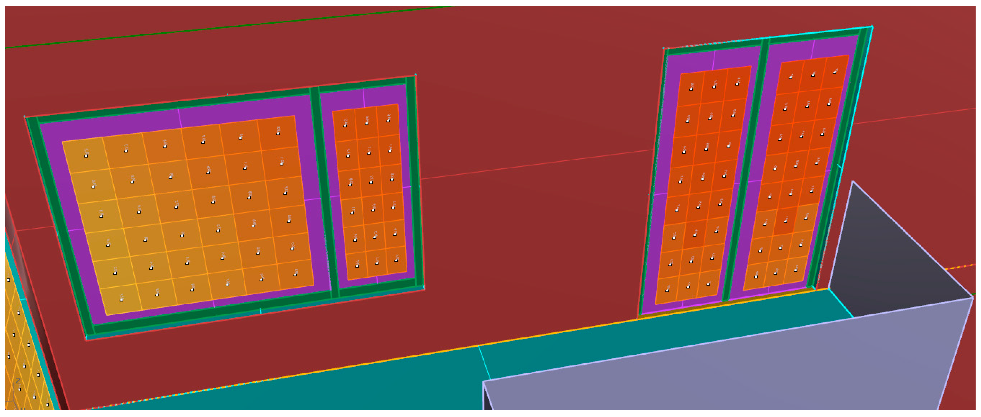
Figure 8.
Calculation grids outside the windows in Rhinoceros.
Figure 8.
Calculation grids outside the windows in Rhinoceros.
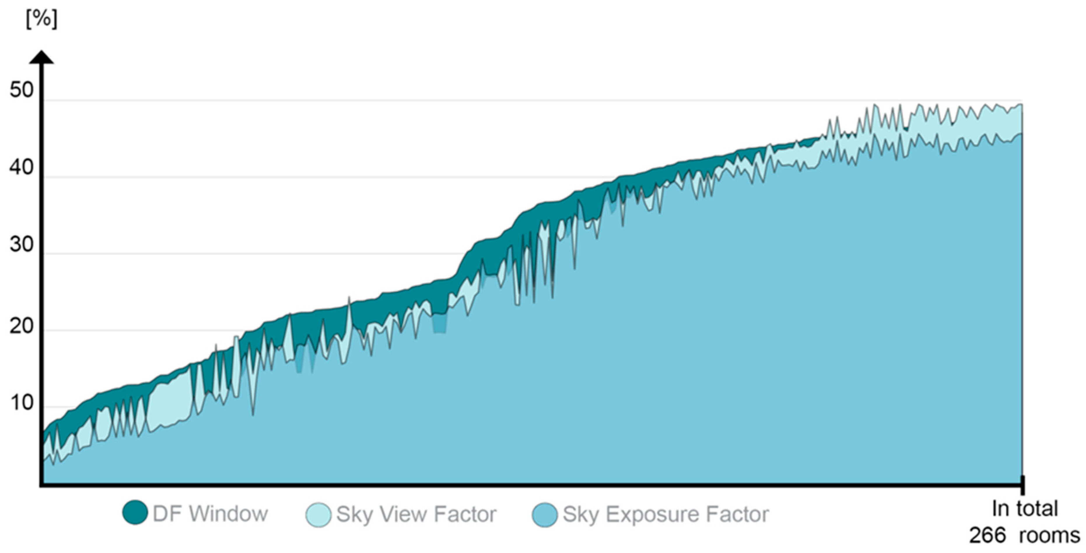
Figure 9.
Daylight factor, sky view factor, and sky exposure factor measured outside the windows. The values are organized after the size of the daylight factor.
Figure 9.
Daylight factor, sky view factor, and sky exposure factor measured outside the windows. The values are organized after the size of the daylight factor.
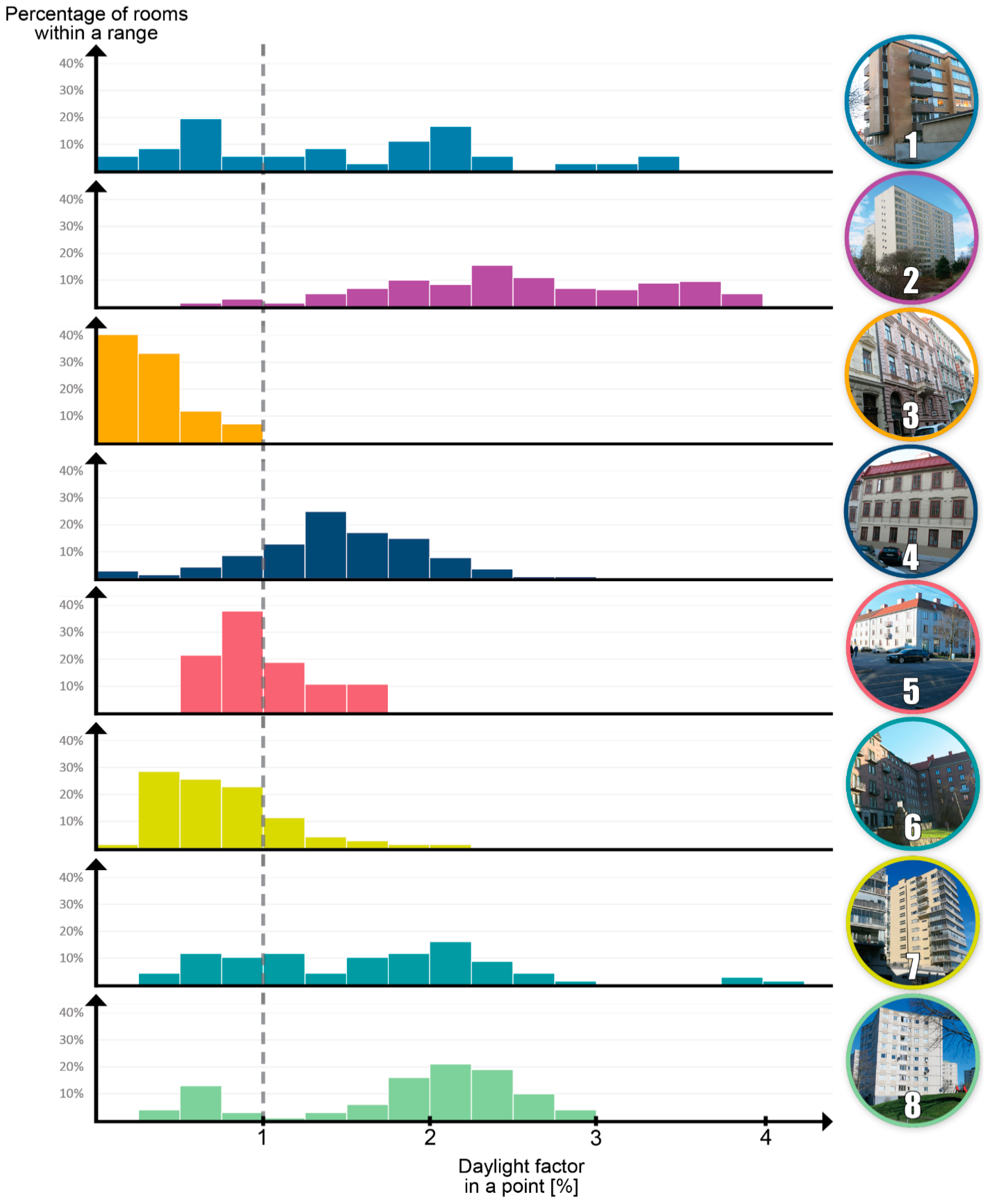
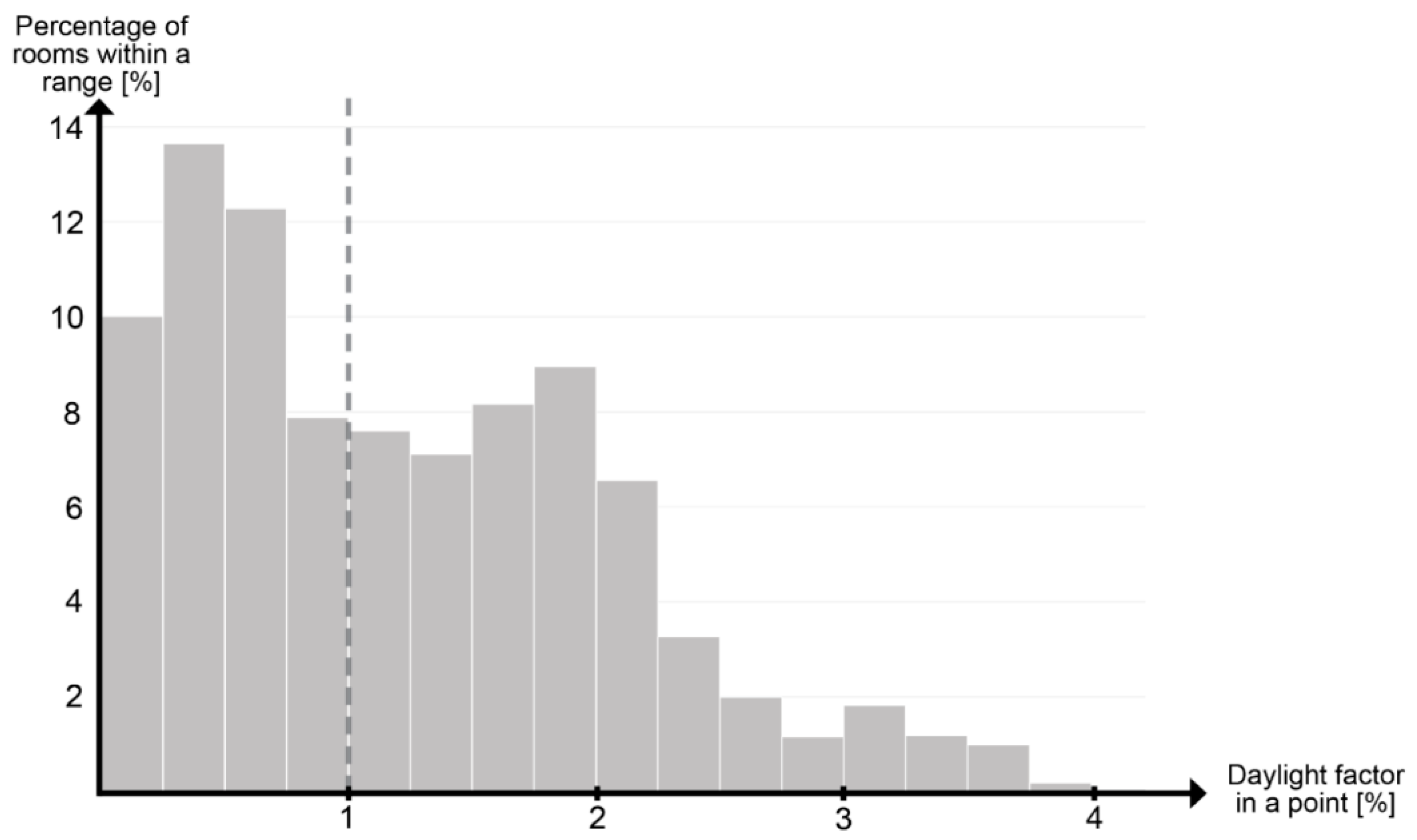
Figure 10.
Distribution of in all the simulated rooms in the residential buildings.
Figure 10.
Distribution of in all the simulated rooms in the residential buildings.
Figure 11.
Distribution of the weighted single-points DF in the residential buildings.
Figure 11.
Distribution of the weighted single-points DF in the residential buildings.
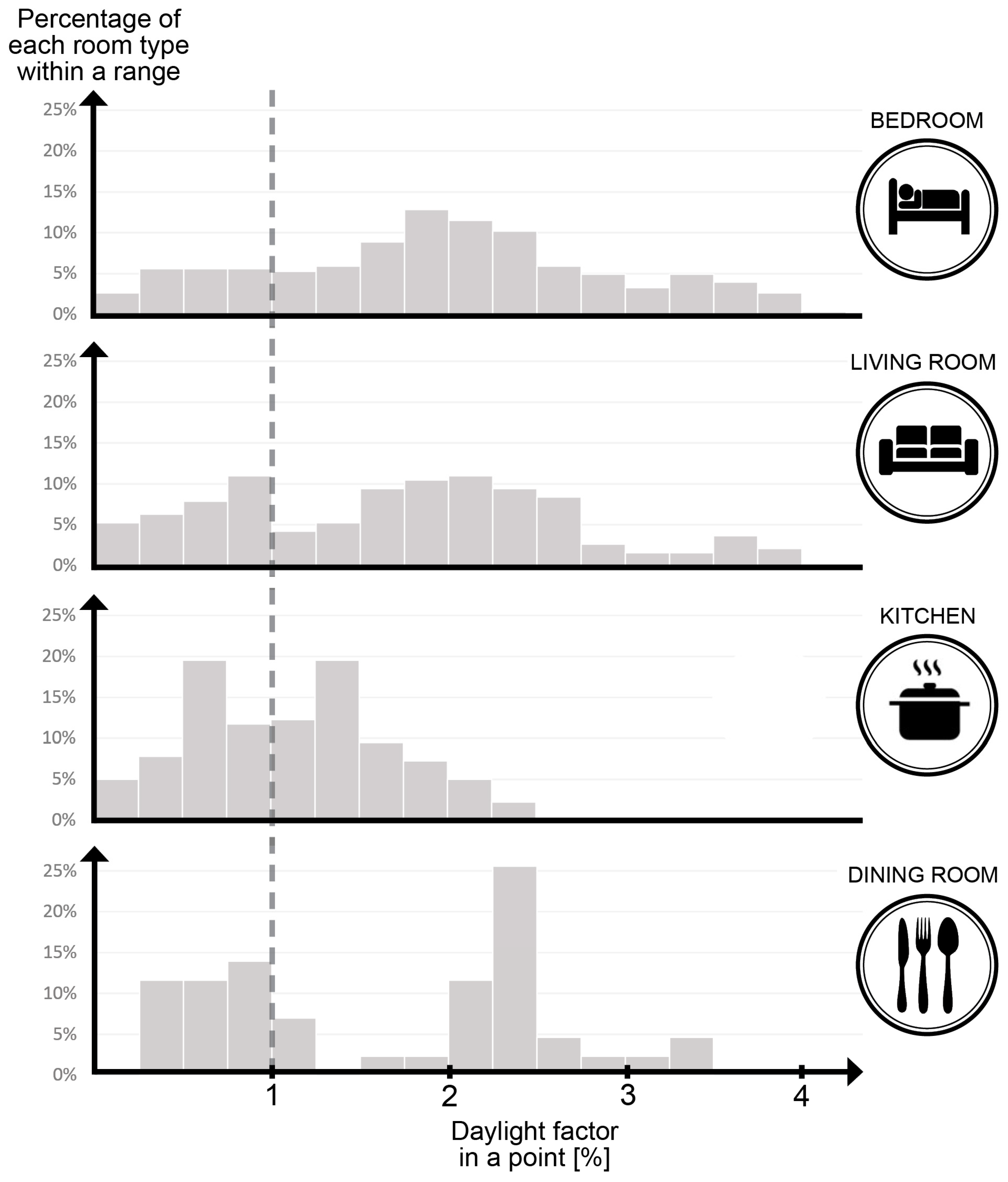
Figure 12.
Distribution of per room type.
Figure 12.
Distribution of per room type.
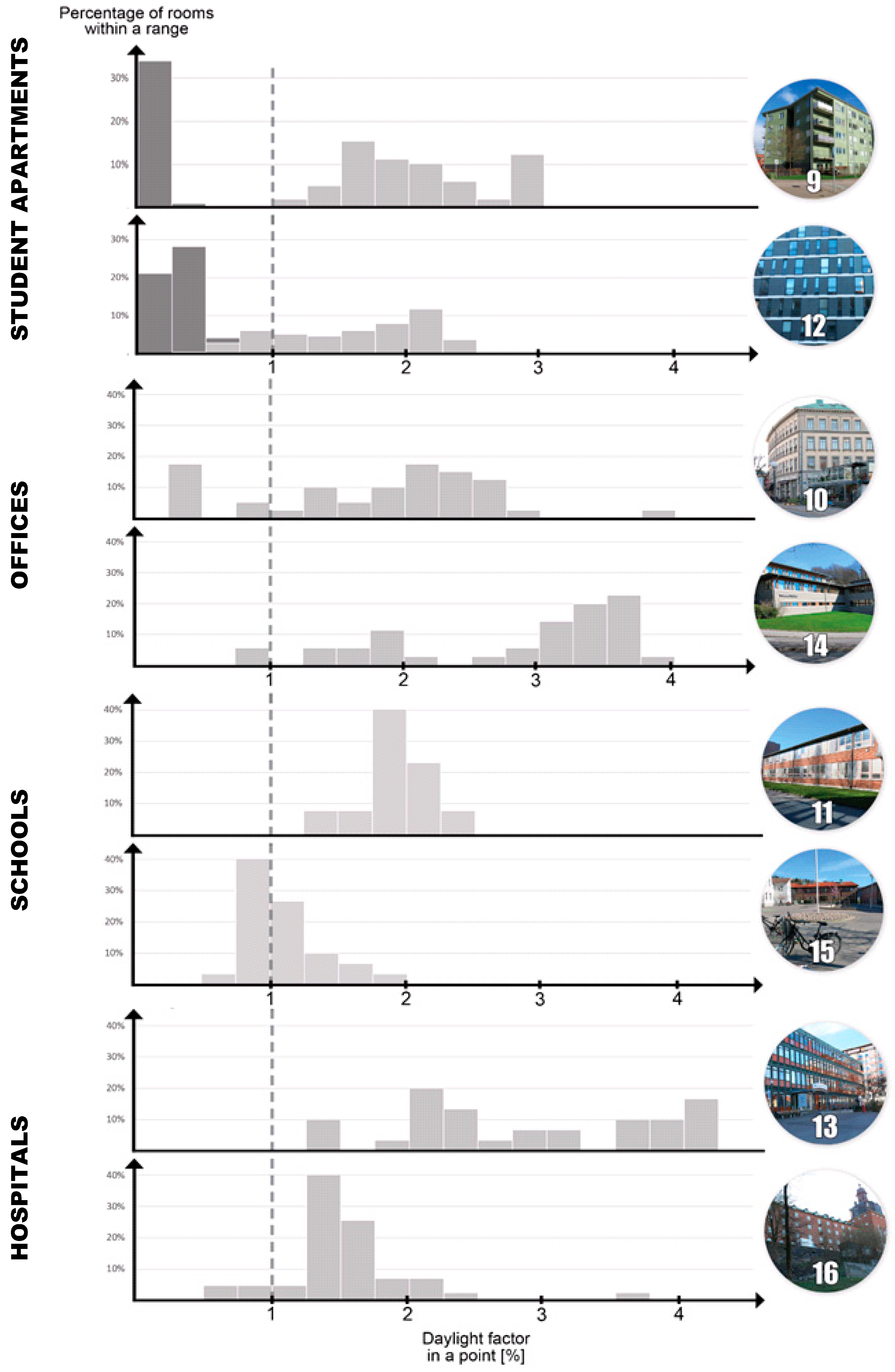
Figure 13.
Distribution of in the student non-residential buildings. For the student apartment buildings, the kitchenettes are marked in dark grey and all other rooms in light grey.
Figure 13.
Distribution of in the student non-residential buildings. For the student apartment buildings, the kitchenettes are marked in dark grey and all other rooms in light grey.
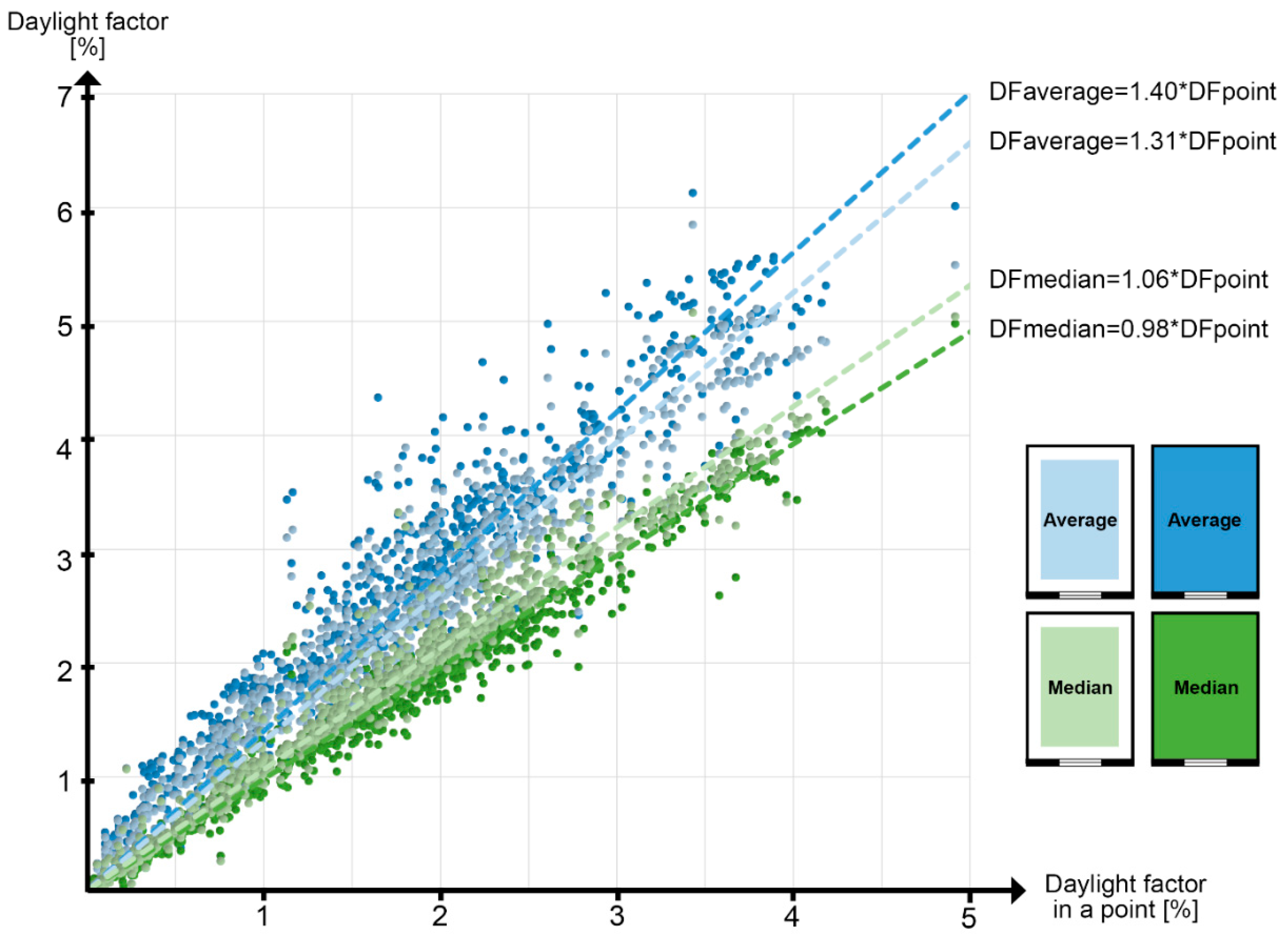
Figure 14.
Comparison between the point-value DFP (horizontal axis) and area-averaged DFs (DFA = DFaverage, DFM = DFmedian, vertical axis), for both full and retracted control surfaces.
Figure 14.
Comparison between the point-value DFP (horizontal axis) and area-averaged DFs (DFA = DFaverage, DFM = DFmedian, vertical axis), for both full and retracted control surfaces.
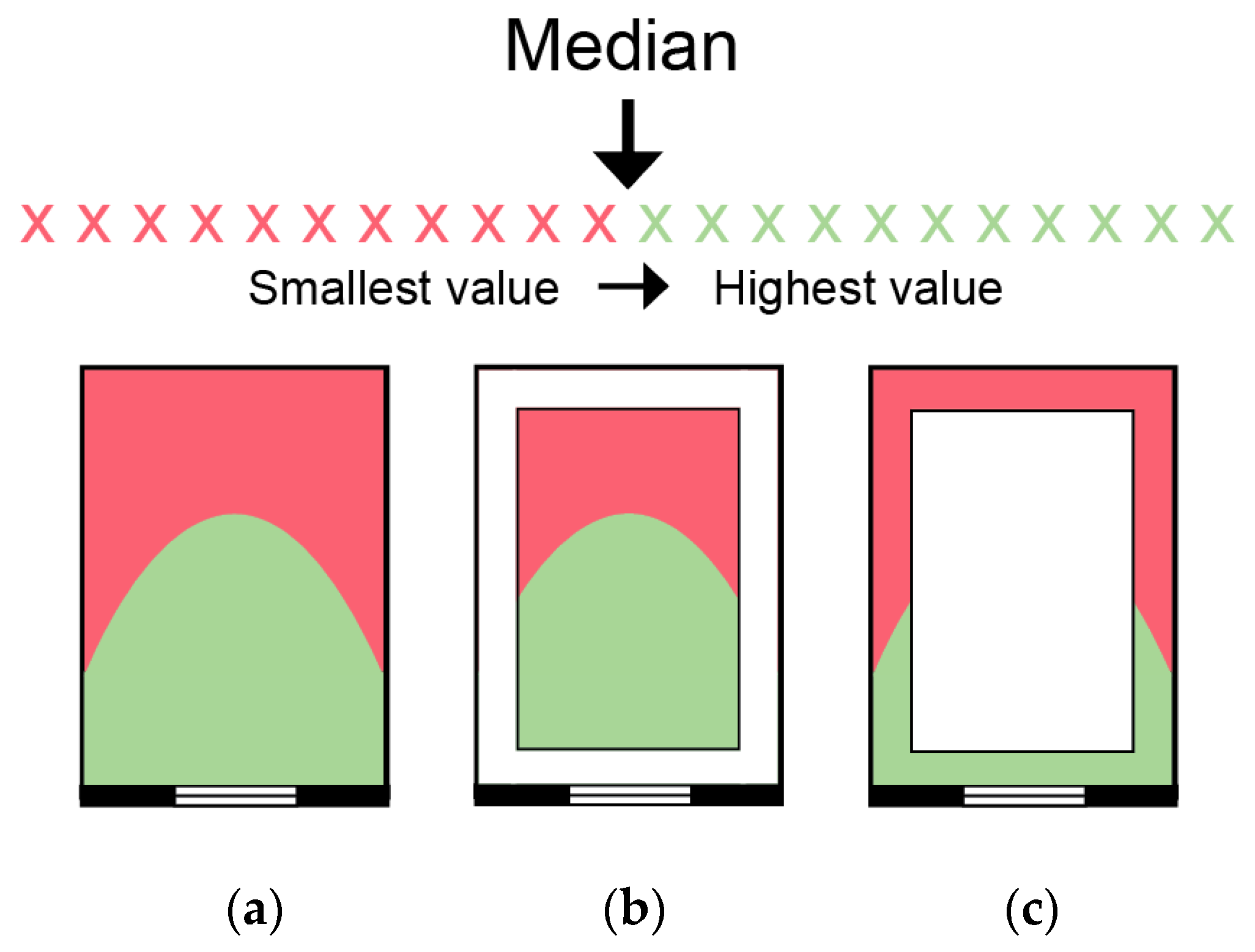
Figure 15.
Impact of the size of a control area on the results of ordinary mean and median DF: (a) the control area covers the whole horizontal section; (b) the control area is retracted 0.5 m from the inner walls; (c) the difference between (a) and (b). The green zone represents the area in the room were the daylight factor is above the median value, while the red zone represents the area in the room were the daylight factor is below the median value.
Figure 16.
Grid-point values of DF arraigned in ascending order, for four different room types. The corresponding average and median values for the same control surfaces are also included.
Figure 16.
Grid-point values of DF arraigned in ascending order, for four different room types. The corresponding average and median values for the same control surfaces are also included.
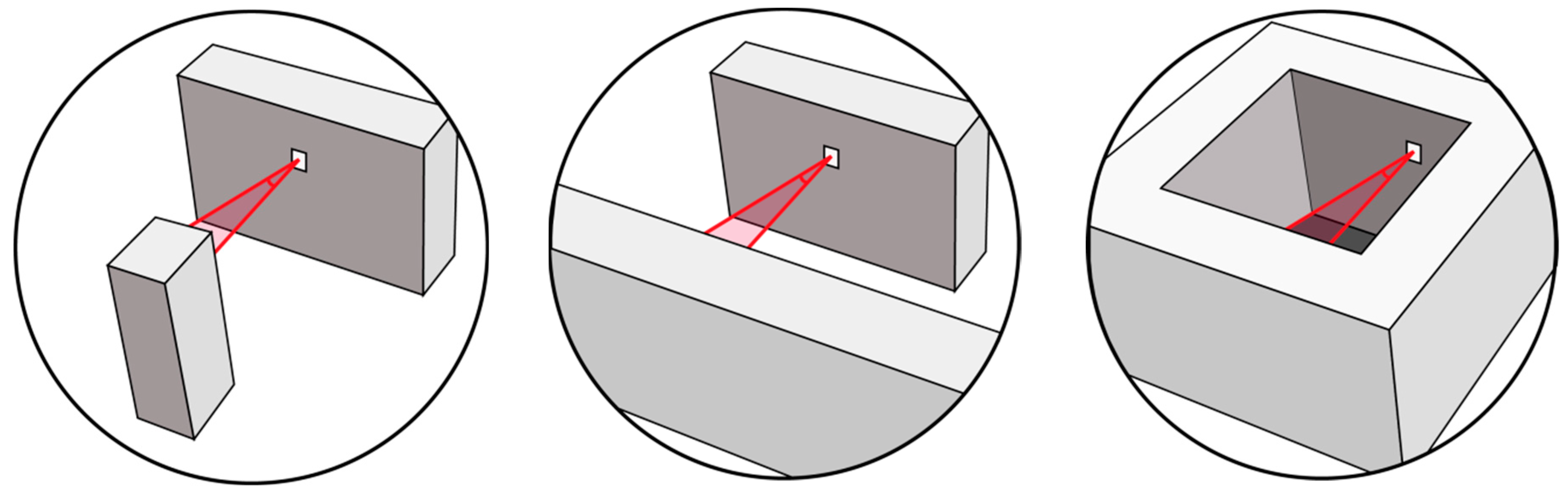
Figure 17.
Three situations for which the AF-method gives the same results (by anticipating the same obstruction angle in front of the window), while the method gives the different results.
Figure 17.
Three situations for which the AF-method gives the same results (by anticipating the same obstruction angle in front of the window), while the method gives the different results.
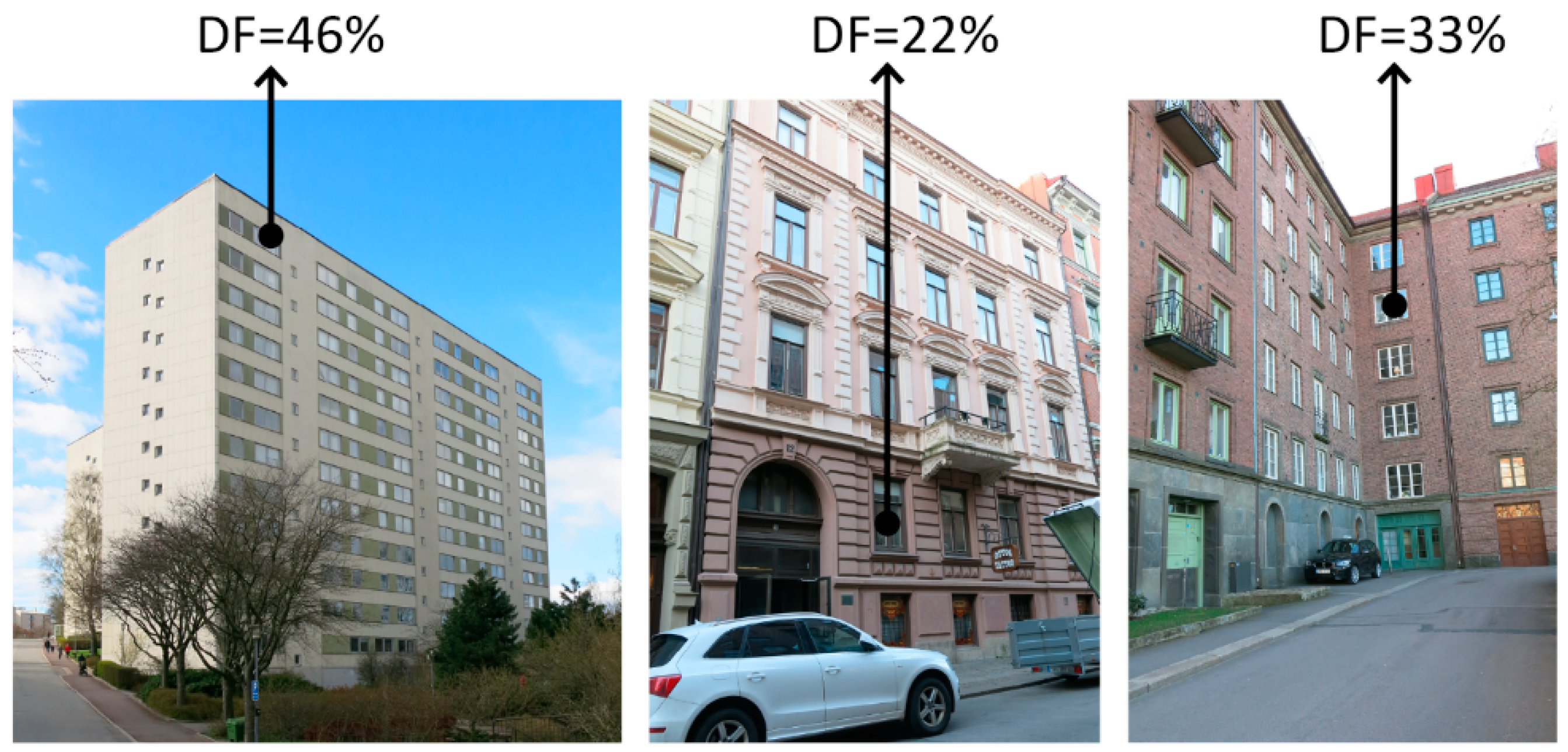
Figure 18.
Examples of different daylight factors outside selected windows in buildings 2, 3, and 6.
Figure 18.
Examples of different daylight factors outside selected windows in buildings 2, 3, and 6.
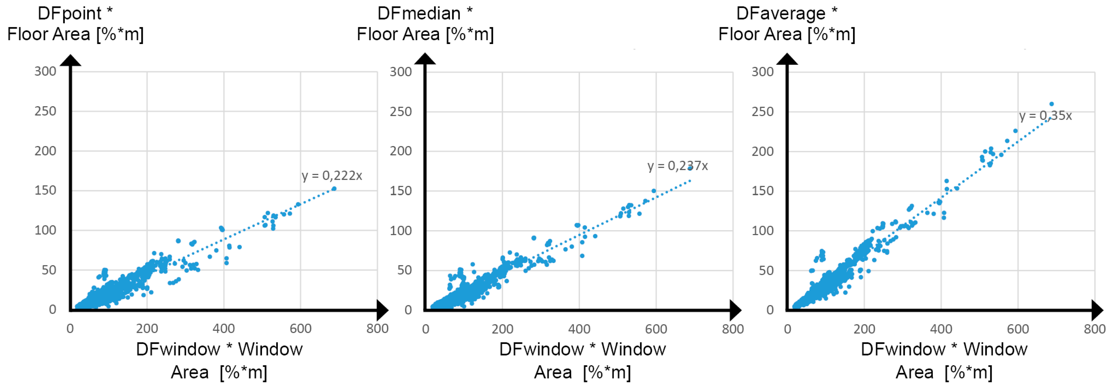
Figure 19.
Correlation between the simulated amount of daylight outside the windows ( multiplied by the window area) and indoors. The latter is given, for three DF indicators, each multiplied by the floor area.
Figure 19.
Correlation between the simulated amount of daylight outside the windows ( multiplied by the window area) and indoors. The latter is given, for three DF indicators, each multiplied by the floor area.
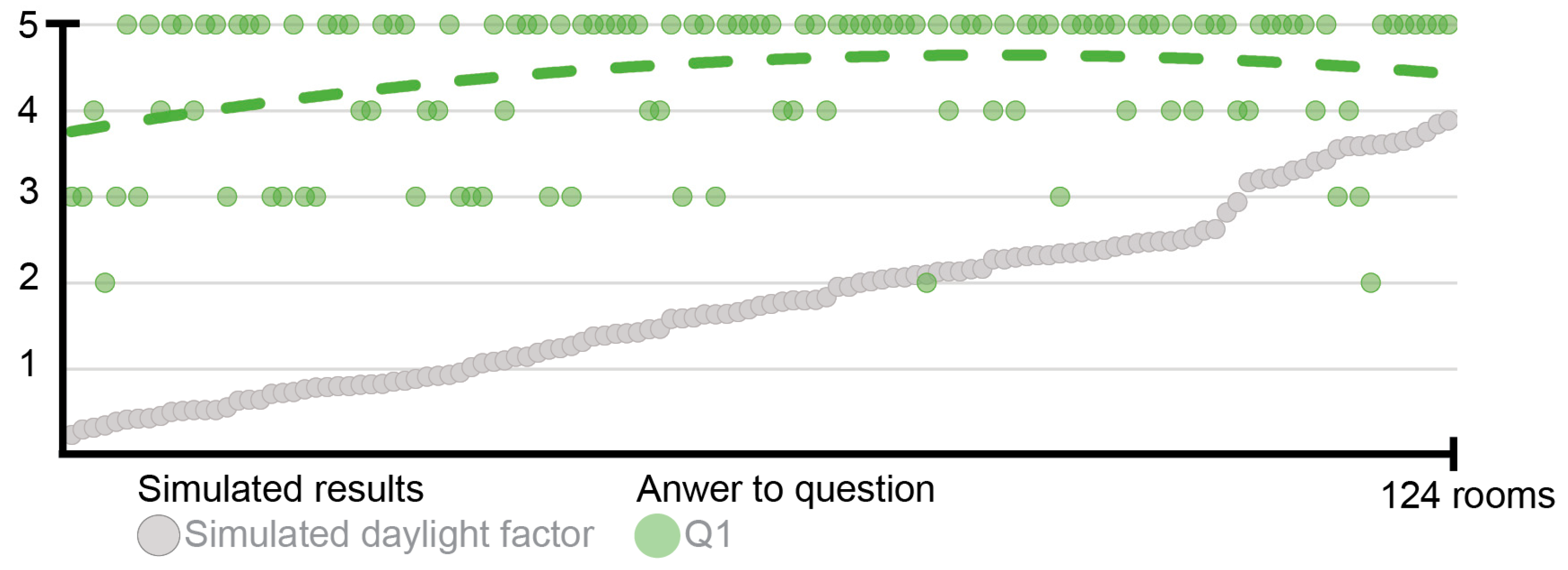
Figure 20.
Simulated single-point DF and the scaled answers to question Q1 from the residents. The dashed line is a fitted polynomial to the answers from residents.
Figure 20.
Simulated single-point DF and the scaled answers to question Q1 from the residents. The dashed line is a fitted polynomial to the answers from residents.
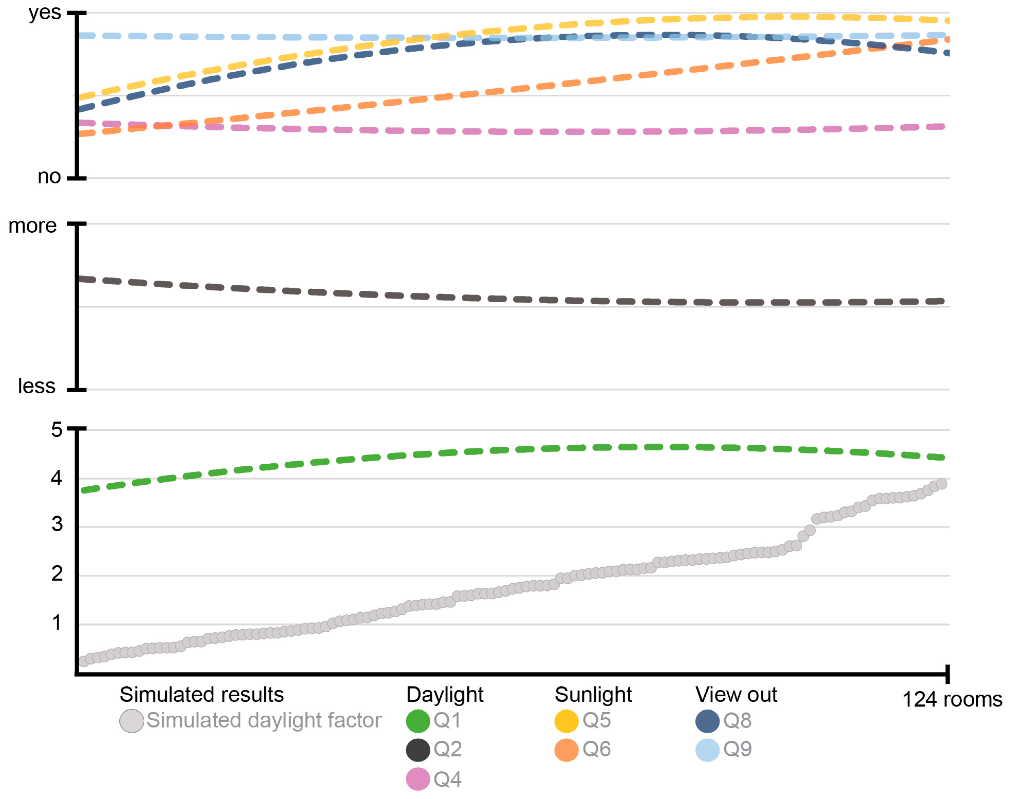
Figure 21.
Trendlines (dashed lines) based on the scaled answers from the survey, compared to the calculated single-point DF for all 124 rooms.
Figure 21.
Trendlines (dashed lines) based on the scaled answers from the survey, compared to the calculated single-point DF for all 124 rooms.
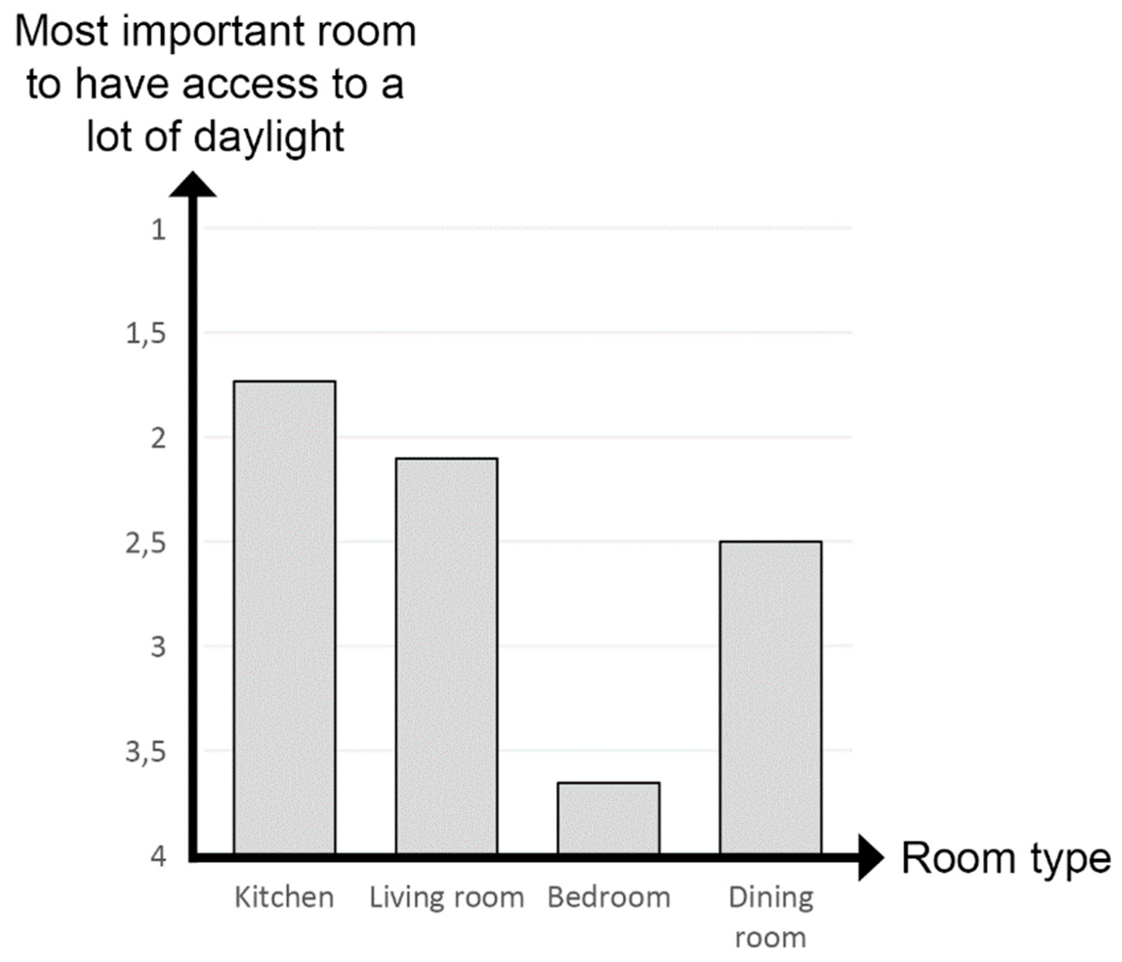
Figure 22.
The residents’ priorities regarding the most important room to have much access to daylight.
Figure 22.
The residents’ priorities regarding the most important room to have much access to daylight.
Table 1.
Main characteristics of the studied buildings. Year = year of construction. Use: R-residential, S-school, O-office, H-hospital, SA-student apartment (micro apartment). Only the floors with the same layout were used, in accordance with the main use of the building.
Table 1.
Main characteristics of the studied buildings. Year = year of construction. Use: R-residential, S-school, O-office, H-hospital, SA-student apartment (micro apartment). Only the floors with the same layout were used, in accordance with the main use of the building.
| ID | Characteristics | Year | Use | Total Number of Floors | Number of Evaluated Floors | Number of Evaluated Rooms |
|---|
| 1 | Elongated apartment block | 1972 | R | 6 | 4 | 36 |
| 2 | Tower block | 1960 | R | 12 | 8 | 200 |
| 3 | Townhouse with a courtyard | 1887 | R | 4 | 4 | 42 |
| 4 | Governor’s house with a courtyard | 1897 | R | 4 | 3 | 140 |
| 5 | Governor’s house with a courtyard | 1923 | R | 3 | 3 | 37 |
| 6 | L-shaped apartment block | 1928 | R | 6 | 5 | 70 |
| 7 | Compact tower block | 2013 | R | 11 | 4 | 68 |
| 8 | Compact tower block | 1960 | R | 10 | 4 | 100 |
| 9 | Compact block | 2004 | SA | 5 | 3 | 97 |
| 10 | Townhouse with two street sides | 1863 | O | 5 | 4 | 47 |
| 11 | Low-rise, elongated | 1962 | S | 2 | 2 | 14 |
| 12 | L-shaped compact block | 2006 | SA | 13 | 5 | 230 |
| 13 | Low-rise compact block | 1966 | H | 4 | 4 | 38 |
| 14 | Low-rise, indented top floor | 2006 | O | 3 | 3 | 36 |
| 15 | U-shaped, low-rise with a school yard | 2001 | S | 2 | 2 | 30 |
| 16 | Block with a tower on one side | 1927 | H | 4 | 3 | 52 |
| | Total | | | | | 1237 |
Table 2.
Reflectance of different objects as used in this study. Reproduced with permission from [
6].
Table 2.
Reflectance of different objects as used in this study. Reproduced with permission from [
6].
| Object | Reflectance | Object | Reflectance |
|---|
| Outside ground | 0.2 | Window frame | 0.8 |
| External façades | 0.3 | Side of window | 0.5 |
| Surrounding buildings and objects | 0.2 | Balcony | 0.3 |
| Floor | 0.3 | Balcony bottom | 0.7 |
| Walls | 0.7 | Water | 0.5 |
| Ceiling | 0.8 | Roof | 0.3 |
Table 3.
Number of distributed and collected surveys for the selected residential buildings.
Table 3.
Number of distributed and collected surveys for the selected residential buildings.
| ID | Number of Distributed Surveys | Number of Collected Surveys | Response Rate |
|---|
| 2 | 36 | 24 | 67% |
| 6 | 15 | 8 | 53% |
| 7 | 16 | 13 | 81% |
| All | 67 | 45 | 67% |
Table 4.
The percentage of rooms with the single-point DF greater than 1% in the residential buildings.
Table 4.
The percentage of rooms with the single-point DF greater than 1% in the residential buildings.
| Building ID | Percentage of All Rooms with a DF > 1% | Average DF for a Building |
|---|
| 1 | 61% | 1.47% |
| 2 | 96% | 2.50% |
| 3 | 0% | 0.31% |
| 4 | 83% | 1.45% |
| 5 | 41% | 1.01% |
| 6 | 21% | 0.74% |
| 7 | 74% | 1.65% |
| 8 | 80% | 1.85% |
| Average for all rooms/buildings | 71% | 1.67% |
Table 5.
Shows all the different room types studied, divided into the four main categories.
Table 5.
Shows all the different room types studied, divided into the four main categories.
| Bedroom | Living Room | Kitchen | Dining Room |
|---|
| Bedroom | Living room | Kitchen | Dining room |
| Small room | Family room | Divided kitchen | Divided dining |
| | Living room/Bedroom | Divided kitchenette | |
| | Living room/Kitchen | Living room/Kitchen | |
Table 6.
Comparison between the results from the AF-method and single-point DF calculations.
Table 6.
Comparison between the results from the AF-method and single-point DF calculations.
| Results for AF | Results for | Percentage of the Studied Rooms | Agreement between the Methods |
|---|
| ≥ 1% | 70% | Yes |
| < 1% | 8% | Yes |
| < 1% | 12% | No |
| ≥ 1% | 10% | No |


