1. Introduction
Nowadays, large-scale and distributed utilization of wind power has been widely developed. In the long run, wind power generation will play an important role in the future energy structure [
1] while constantly improving its own shortcomings such as wind turbine noise impact [
2,
3,
4,
5] and wind energy volatility. With the rapid growth of the proportion of grid-connected wind power, whether for a large-grid or for a micro-grid, the volatility of primary wind energy is usually a concern for the safe and economic operation of the power grid. Against this background, wind power prediction is very helpful to enhance our knowledge of the wind energy variation and help increase the controllability of wind power. As a result, it has become very important for the modern wind power industry [
6].
Wind power prediction can be realized with different time scales such as ultra-short-term, short- term, medium-term and long-term, etc. Among them, short-term prediction of wind power for a wind farm has been popularly studied [
7], serving for day-ahead dispatching, pre-dispatching or on-line dispatching. Especially, due to increasing accuracy [
8], numerical weather prediction provides more support for the power prediction of wind farms in a wide area. However, for a wind turbine at a specific-site, the spatial scale is too small and numerical weather prediction information become inaccurate. Considering the requirements such as optimal control of wind turbines, economic power dispatching of wind farms and auxiliary peak/frequency modulation service, etc., the ultra-short-term power prediction of wind turbines has attracted more and more attention. This is the main object of study in this paper.
Due to the fact accurate numerical weather prediction information is not easily accessible for wind turbines, stepwise prediction is very suitable, usually including wind speed prediction and WTPC modeling. It is flexible enough to identify the accuracy of each step. In [
6,
9], stepwise prediction of wind power using predicted wind speed and WTPC was clearly introduced. Nevertheless, in many publications, wind speed prediction and WTPC modeling are studied separately.
In [
10], Hu, et al., used generalized principal component analysis for the classification of wind patterns. Support vector regression was utilized for local modeling and a switching strategy was proposed for global short-term prediction. In [
11], a time adaptive filter-based empirical mode decomposition was used to decompose wind speed series into several intrinsic modes and global short-term predictions were realized through assembled calculation of local models via an extreme learning machine approach. In the above studies, short-term point prediction of wind speed was the main concern and attention was paid to the classification of hidden wind speed patterns. Thereafter, the randomness of wind speed is examined to yield interval predictions. In [
12], an empirical wavelet transform was employed to extract meaningful information from wind speed series and a hybrid GPR model was built for short-term interval prediction of wind speeds. Using similar schemes, in [
13,
14], variational mode decomposition was combined with relevance vector machine and low rank multi-kernel ridge regression to realize short-term interval predictions of wind speed. However, ultra-short-term interval prediction of wind speed hasn’t been studied. Besides, the mean square error is always used as the objective for parameter optimization of prediction algorithms. In [
15], evaluation indexes for interval prediction performance of wind speed were defined to form a multi-objective framework. However, the point prediction performance wasn’t involved. Then, separate optimization of point or interval prediction performance may worsen that of the other one.
WTPC is a kind of steady-state description of the power generation characteristics of a wind turbine. Different from the designed WTPC given by the original equipment manufacturer (OEM), the actual data distribution of wind speed and power shows a banding shape influenced by many random factors. Using parametric or non-parametric methods, WTPC modeling has been widely studied [
16,
17]. Especially, uncertainty modeling of WTPC has been paid certain attention. In [
18,
19], using Gaussian and conditional kernel density estimation, respectively, joint probability distributions of wind speed and power were established, whereas only point estimation of WTPC was discussed. In [
20,
21], Bai, et al., adopted conditional copula to establish the joint probability distribution of wind speed and power, where only interval estimation of WTPC was discussed. In [
22], fuzzy cluster, BP neural network and Monte-Carlo algorithms were compared to obtain probabilistic WTPC models. According to these references, joint point-interval estimation of WTPC has not been clearly claimed. Furthermore, the relationship between point and interval estimation has not been revealed. Meanwhile, how to evaluate and optimize the joint point-interval estimation performance still lacks relevant research.
Affected by stochastic wind energy and complex interference factors, uncertainty prediction of wind power is necessary [
23,
24]. If a stepwise procedure is executed, how to deal with the sequential uncertainties of wind speed prediction and WTPC modeling is a critical question. In [
25], Liu, et al., studied interval prediction of wind power for a wind farm considering the uncertainty of wind speed prediction via ARMA-GARCH and the operation probability of wind turbines. It suggested the necessity of considering sequential uncertainties for wind power prediction. However, it is different from the ultra-short-term prediction of wind power for a wind turbine where both the uncertainties of wind speed prediction and WTPC modeling need to be considered.
Comparing different interval modeling methods, two classes can be obtained. One class is based on conditional probability distribution of output against inputs where regression values in view of conditional expectation and boundaries under certain confidence degree can be obtained. The methods such as conditional kernel density estimation, conditional copula, GPR and relevant vector machine belong to this class, where point and interval estimation can be jointly realized. The other class is based on conditional probability of prediction error against predicted values using normal point regression algorithms. Confidence boundaries of prediction error can be also yielded [
26,
27]. Under different application scenarios such as single-step or multi-step prediction of wind power, appropriate method should be selected to get reasonable description form of interval prediction.
Considering the feasibility of ultra-short-term wind power prediction via a stepwise procedure, GPR is chosen as the main algorithm for wind speed prediction and WTPC modeling. On this basis, the main contributions of this paper may be listed as follows:
The concept of TIG is defined to build an input-output matrix for ultra-short-term wind speed prediction. A PCA-clustering scheme is proposed to extract hidden wind patterns in TIGs.
Joint point-interval prediction of wind power is clearly claimed and studied via GPR. Theoretical support for uncertainty enlargement due to sequential uncertainties during stepwise procedure is deduced.
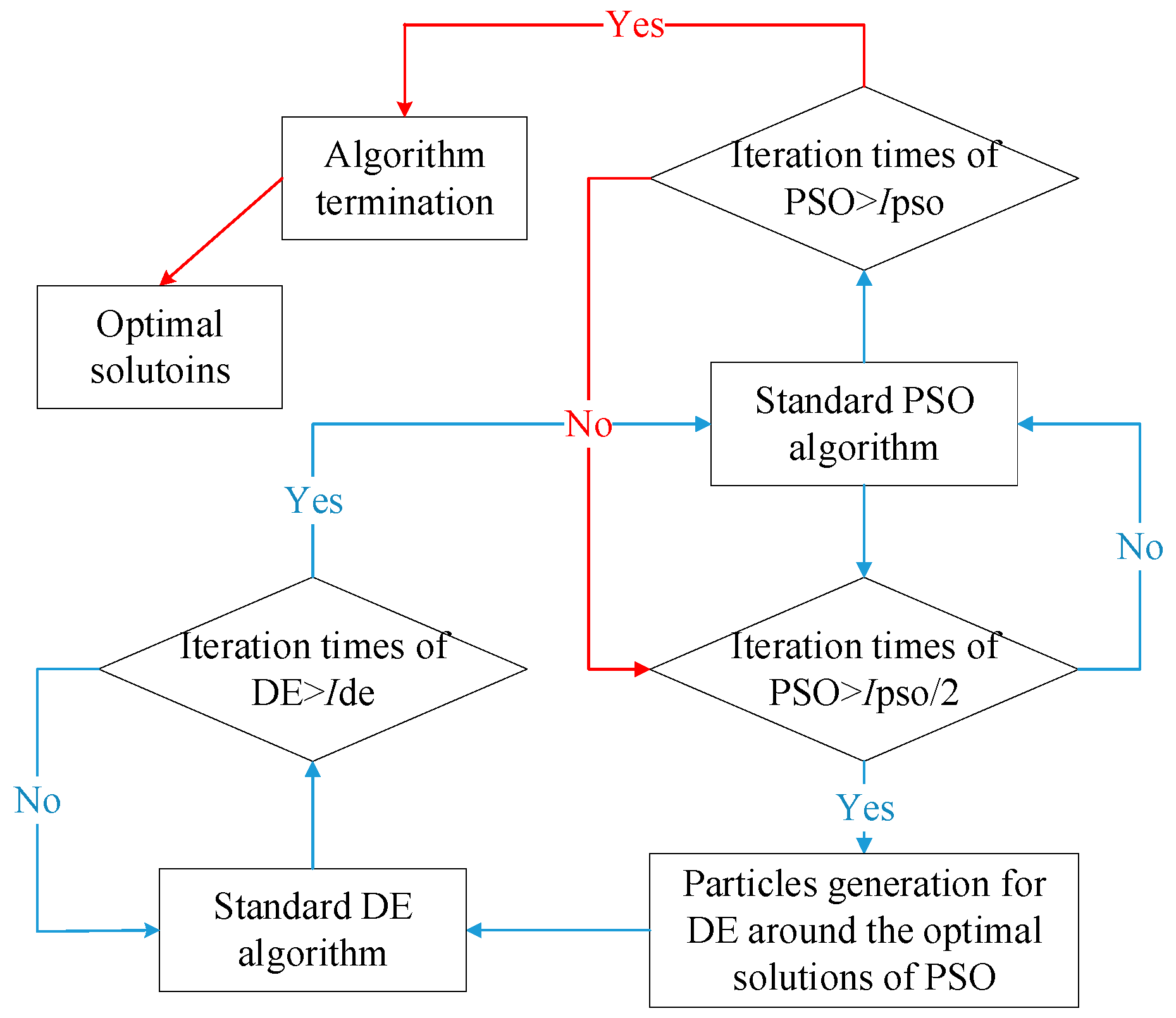
Normalized and comprehensive evaluation indexes for joint point-interval estimation performance are defined systematically. Hybrid PSO-DE algorithm and K-CV method are used to obtain better and more stable performance.
After single-step or receding multi-step wind speed prediction, uncertainty enlargement effects during stepwise wind power prediction is revealed and validated using parametric and non-parametric interval modeling methods.
The rest of the paper is organized as follows:
Section 2 presents the establishment of a multi-model structure for wind speed prediction.
Section 3 completely proposes the joint point-interval prediction of wind power via stepwise procedure.
Section 4 defines normalized and comprehensive evaluation indexes for joint point-interval prediction of wind power while evolutionary updating mechanism is raised. Simulation and analysis are executed in
Section 5.
Section 6 concludes the paper.
2. Establishment of Multi-Model Structure for Wind Speed Prediction
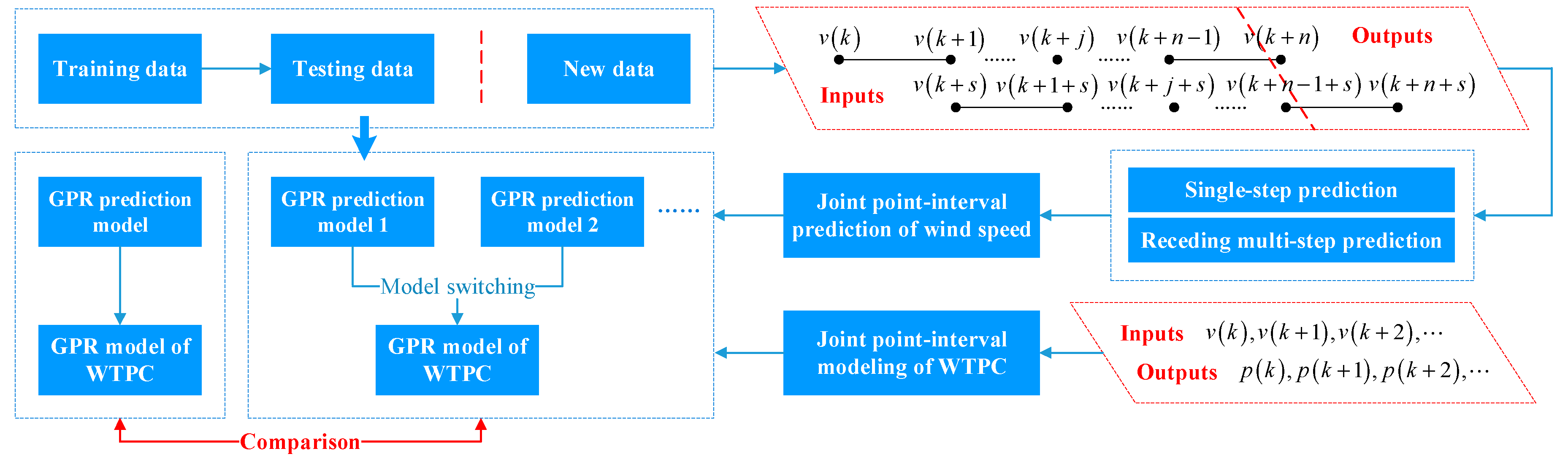
2.1. Formation of Input-Ouput Matrix
To realize receding wind power prediction of a single wind turbine, a stepwise procedure is adopted in this paper, including receding wind speed prediction and WTPC modeling. We set the sampling period as
TV and split the wind speed time series into many segments, where a segment is defined by
Vi = [
vi1,
vi2, …,
vij, …,
vin] = [
vi(
k),
vi(
k + 1), …,
vi(
k +
j), …,
vi(
k +
n − 1)] where
Vi+1 = [
vi(
k +
s),
vi(
k + 1 +
s), …,
vi(
k +
j + s), …,
vi(
k +
n − 1 +
s)] (1 ≤
s ≤
n). Different values of
s mean different ways of sampling the data.
Vi is the
i-th wind speed segment with
n elements sequentially distributed along
n time instants.
Vi is a TIG in time-domain space. Assume
m segments can be obtained, making up the following matrix
V.
For V, rows are seen as r repetitions. Columns from 1 to (n − 1) are seen as inputs, shown by Vi,In = [vi1, vi2, …, vij, …, vin−1]. The n-th column is seen as output, shown by Vi,Out = vin (i = 1, 2,…, r; j = 1, 2,…, n). As a result, for receding wind speed prediction, V is the input-output matrix. Relatively, WTPC modeling is independent of receding prediction of wind speed. Only wind speed and power data are needed as the input and output of WTPC modeling.
2.2. Feature Extraction of Hidden Wind Speed Patterns
For a wind turbine at a specific site, the wind conditions may change with the seasons, wind directions and spatial terrains. It is intuitive that prediction accuracy may be raised under the same wind conditions. However, it is not certain for different prediction algorithms. In this subsection, wind speed is used to represent wind conditions and hidden wind speed patterns are extracted.
Using TIGs of wind speed, PCA [
28] is an effective post-processing manner to extract features of TIGs and to form feature-information-granules. It is convenient for dimensionality reduction of high-dimensional data via a statistical procedure. Then, noise and unimportant features can be removed to enhance the calculation efficiency. It uses an orthogonal transformation to convert a set of observations of possibly correlated variables into a set of values of linearly uncorrelated variables called principal components where the first principal component has the largest possible variance and each succeeding component in turn has the highest variance possible under the constraint that it is orthogonal to the preceding components. Each component vector is a linear combination of input variables and all component vectors form an uncorrelated orthogonal basis set.
Based on Equation (1), we remove the column mean values of
V and it becomes a column-wise zero empirical mean. Then, PCA is executed and
p new features can be obtained where
xil =
ω1l∙
vi1 +
ω2l∙
vi2 +…+
ωjl∙
vij +…+
ωnl∙
vin =
ωl∙
ViT(
ωl = [
ω1l,
ω2l,…,
ωjl,…,
ωnl];
l = 1, 2,…,
h). As a result, feature matrix can be represented as follows:
If n is chosen to be much bigger than h, the dimensionality reduction effect becomes obvious. This provides good convenience for the subsequent calculation.
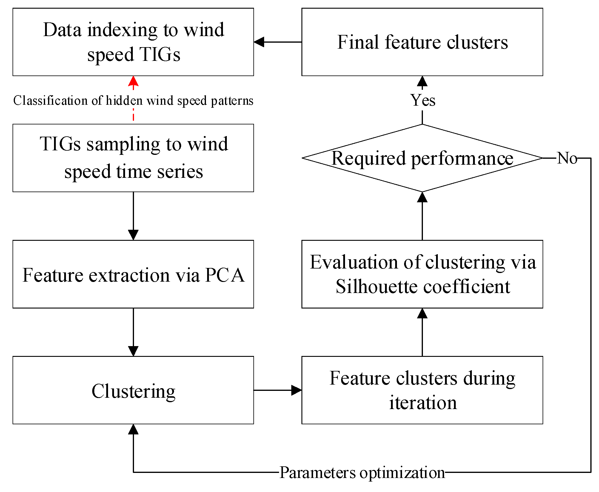
2.3. Classification of Extracted Features via Clustering
Extracted features represent the main hidden information in TIGs. To classify them, an adaptive classification strategy via clustering is presented here. Firstly, unsupervised clustering algorithms such as K-medoids clustering, fuzzy C-means (FCM) clustering, Gaussian-mixture-model (GMM) clustering and ADAP clustering, are adopted and compared. Secondly, to evaluate clustering effects, the silhouette coefficient is used considering inter-cluster and intra-cluster effects which has better and more balanced evaluation performance than other evaluation indexes such as Davies-Bouldin index and Dunn-Validity index. The silhouette coefficient range is [−1,1] and it measures how similar an object is to its own cluster compared to other clusters. A high value suggests that the object is well suited to its own cluster and poorly suited to the neighboring clusters.
Silhouette coefficients can be calculated with any distance metric including Euclidean distance and Manhattan distance, etc. Define
dintra(
ui) as average distance between point
ui and all other points within the same cluster. Define
dintel(
ui) as average distance between point
ui and all points in any other cluster. Then, the silhouette coefficient [
29] is calculated by:
where the value close to 1 means that the point is appropriately clustered; the value close to −1 means that the point would be more appropriately clustered in its neighbouring cluster; a zero value means that the point is on the border of two clusters. Using the silhouette coefficient, the effects of different clustering algorithms can be evaluated and even optimized by the intelligent evolutionary algorithms such as genetic algorithm (GA), PSO and DE algorithms. Finally, wind speed TIGs can be classified via clustering. Besides, new input TIGs can also be classified into reasonable clusters via the silhouette coefficient. It provides a judgment for model switching under a multi-model structure.
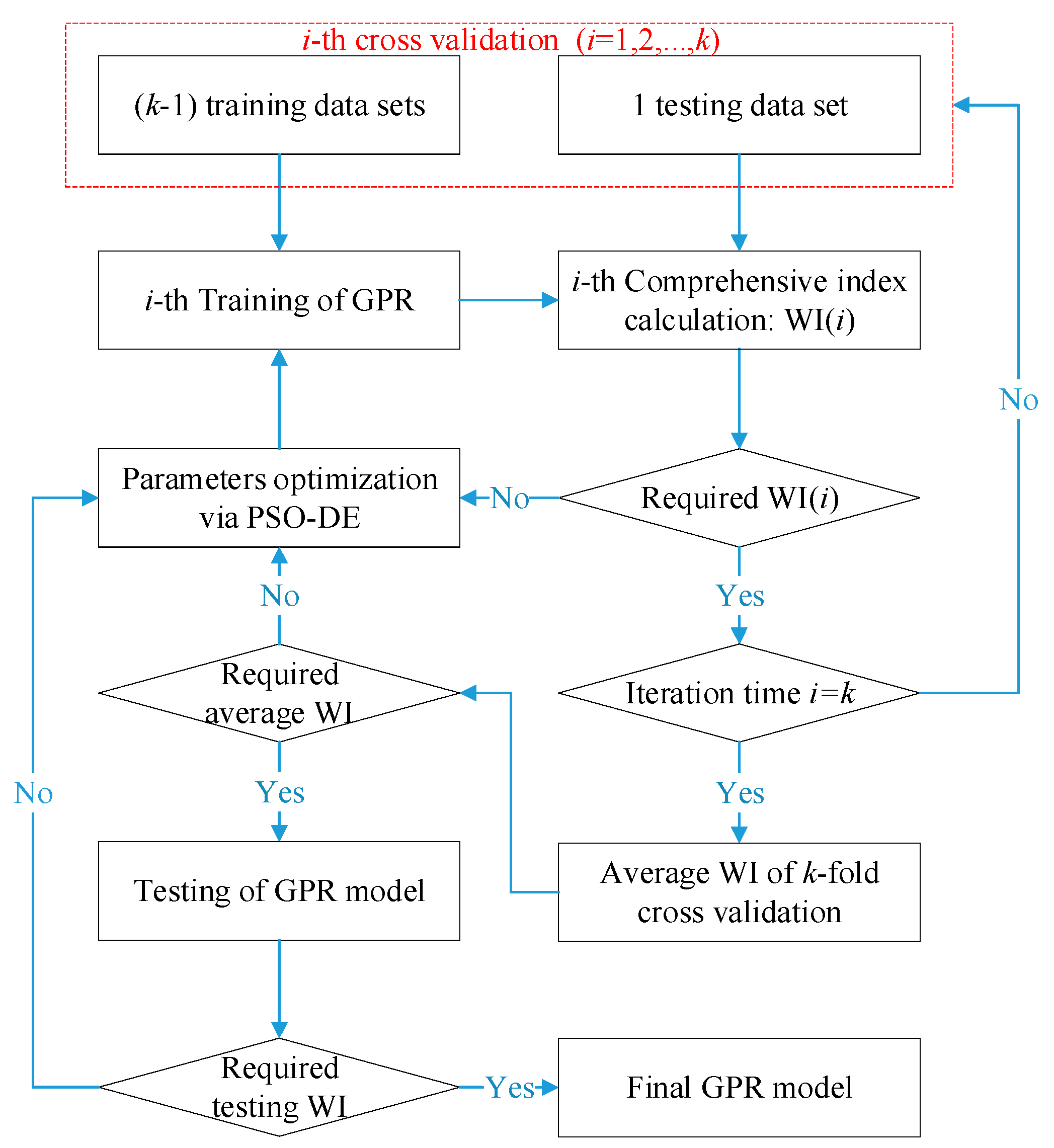
Overall, as shown in
Figure 1, the classification scheme of hidden wind speed patterns is wholly proposed to establish multi-model structure for receding wind speed prediction.
5. Simulations
Based on the data from the supervisory control and data acquisition (SCADA) system of a wind farm located in northern China, wind speed and power data are acquired and preprocessed for prediction. In the wind farm, 1.5 megawatt wind turbines with variable-speed variable-pitch ability are mainly used. The sampling period of the data is 15 min, which is also the time interval of single-step prediction.
5.1. Decision of TIG Length for Wind Speed Prediction
TIG length predetermines the input dimensions of GPR. Herein, single-step prediction of wind speed using different TIG lengths are tested to select an appropriate length. We arbitrarily choose wind speed data with a sampling period of 15 min. Two thousand (2000) data points are randomly selected for training (1600 points) and testing (400 points). Besides, for GPR modeling, type of basis-function is pure quadratic and the type of kernel-function is square exponential, defined as follows:
where
σl is the characteristic length scale.
σf is the signal standard deviation. Mean square error (MSE) is used for optimization the parameters such as
σ,
σl and
σf. Indexes such as NRMSE, NMACE, NPIAW and WI are used for evaluation where weights are all 1/3, as shown in
Table 1.
Two samples are randomly selected for testing under each TIG length. From
Table 1, NMACE varies obviously while the indexes of NRMSE and NPIAW perform relatively stable. When the TIG length is greater than or equal to 6, their WIs become stable at the same bound level. To avoid unnecessary computational burden, 6 is selected as the TIG length in this paper.
5.2. Necessity of Comprehensive Optimization Based on WI
Normally, the parameters of GPR are optimized using MSE of point prediction as the objective. This doesn’t consider interval performance. In extreme cases, excessively optimizing MSE may cause performance deterioration of the interval prediction. Thus, in this subsection, different objectives are tested for wind speed prediction and WTPC modeling using GPR where PSO-DE is adopted.
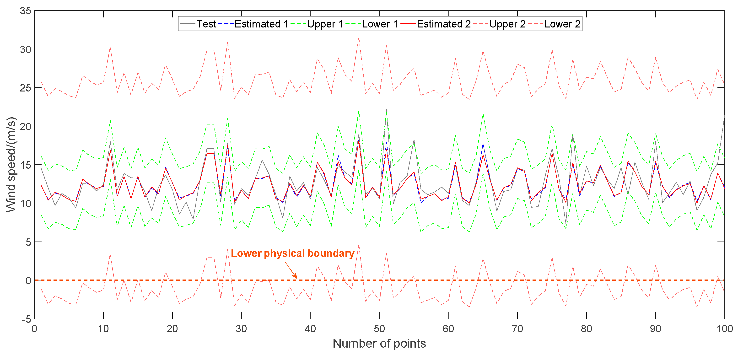
For wind speed prediction via GPR, testing results are shown in
Table 2 and
Figure 6. In
Figure 6, ‘Estimated 1’, ‘Upper 1’ and ‘Lower 1’ are results using WI as objective. ‘Estimated 2’, ‘Upper 2’ and ‘Lower 2’ are results using MSE as objective. Just using MSE as optimization objective, its point prediction index, NRMSE, is very close with that of WI. However, their interval prediction indexes, NMACE and NPIAW are distinguished from each other greatly. As a result, their WIs are also different. These results reflect a truth that using WI as objective is necessary for parameter optimization of GPR when predicting wind speed. Of course, lower boundaries in
Figure 6 are retained to show interval modeling effect of WTPC from a statistical view. In actual, physical boundaries of wind speed should be considered. Usually, zero line is the lower physical boundary of wind speed whereas upper boundary of GPR fulfills its physical meaning.
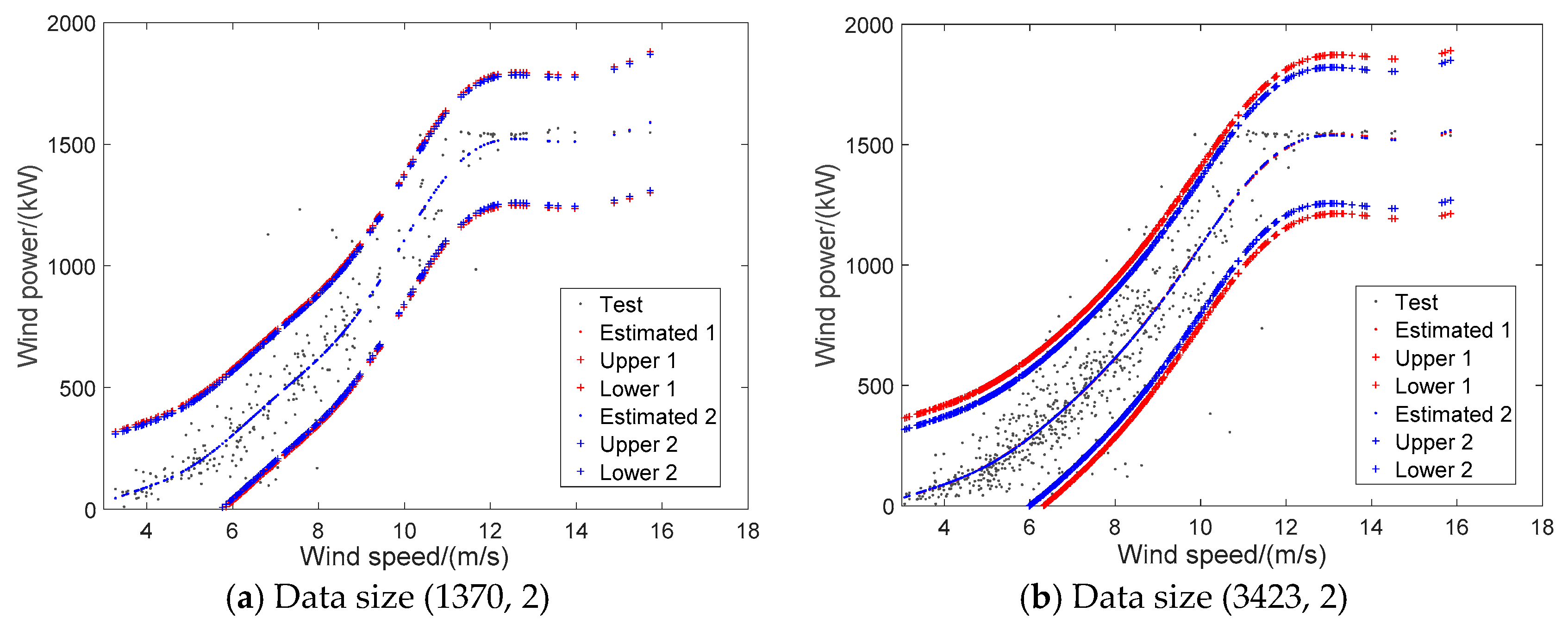
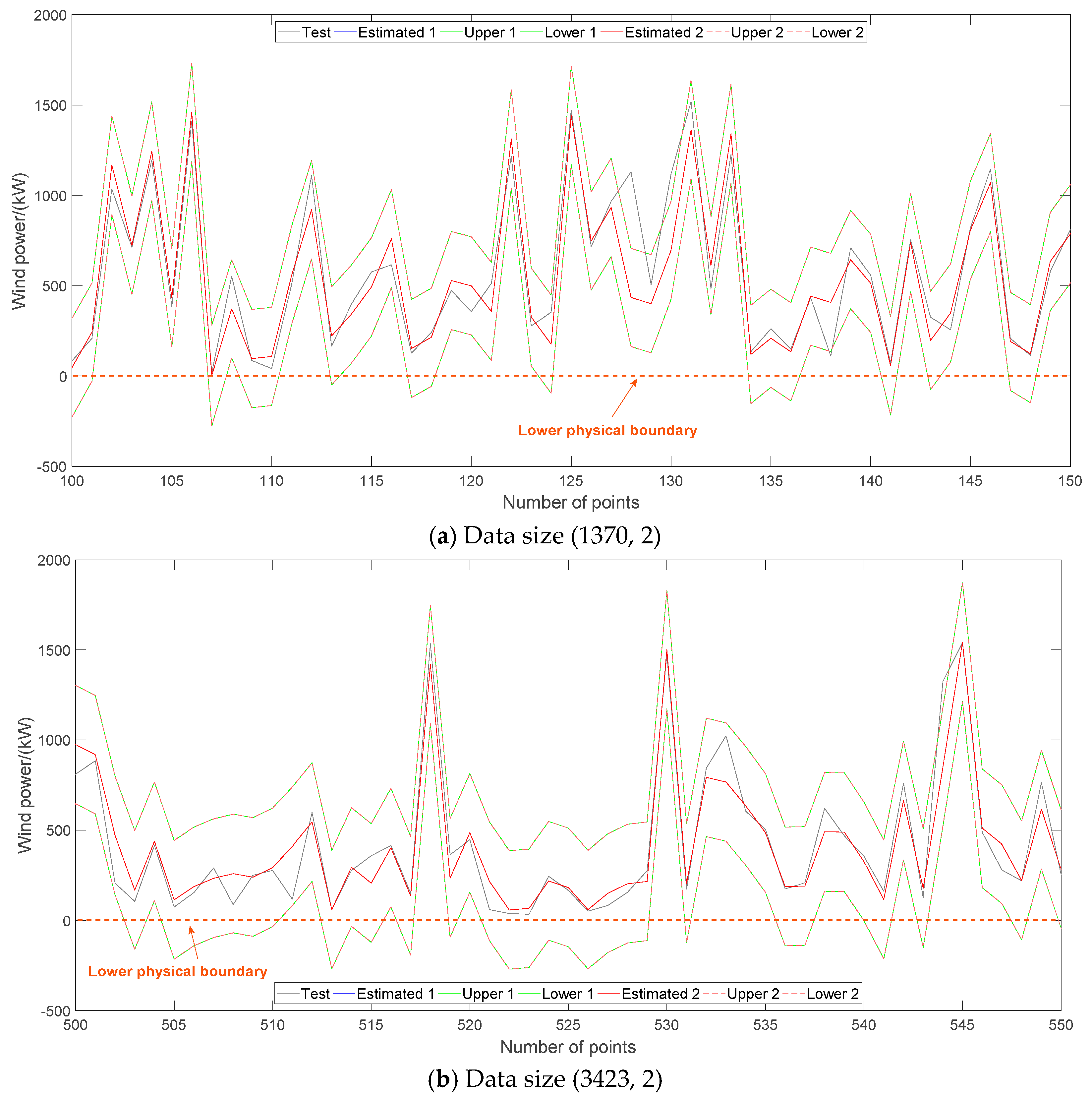
For WTPC modeling via GPR, testing results are shown in
Table 3,
Figure 7 and
Figure 8. In
Figure 7 and
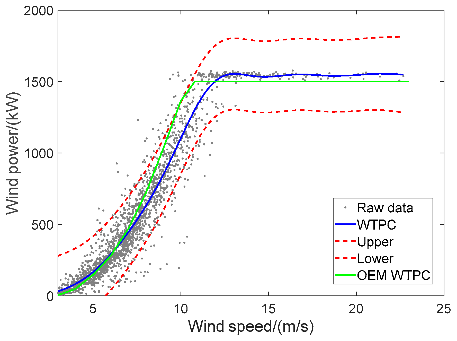
Figure 8, ‘Estimated 1’, ‘Upper 1’ and ‘Lower 1’ are results using WI as objective. ‘Estimated 2’, ‘Upper 2’ and ‘Lower 2’ are results using MSE as objective. It can be found that taking MSE or WI as objective has very little influence on modeling performance. Moreover, the two objectives have very close modeling effects, including both the point and interval indexes. Thus, it is unnecessary to distinguish the usage of MSE and WI for parameter optimization of WTPC modeling via GPR. In
Figure 7, wind power exceeding cut-in wind speed 3 m/s is shown. In
Figure 8, physical boundaries of wind power should be also paid attention where zero line is the lower physical boundary whereas upper boundary of GPR fulfills its physical meaning.
5.3. Establishment and Testing of Multi-Model Structure via PCA-Clustering Scheme
Intuitively, partition of wind speed patterns can raise prediction accuracy of wind speed. However, under the Bayesian framework of GPR, it will be seriously tested in this subsection. To identify the hidden wind speed patterns effectively, PCA-clustering strategy is presented. Herein, the total size of the data sample is (6300, 6) where the input is five dimensional and the output is one dimensional. After feature extraction, three dominant features are used for clustering, where K-medoids, ADAP, FCM and GMM clustering methods are compared. The results are shown in
Table 4 using the silhouette coefficient as evaluation index. Concerning consumed time,
K-medoids, FCM and GMM performs well, whereas ADAP is very time consuming. When the cluster number equals 2, all methods have similar silhouette coefficients. However, the data uniformities of the clusters are different. For
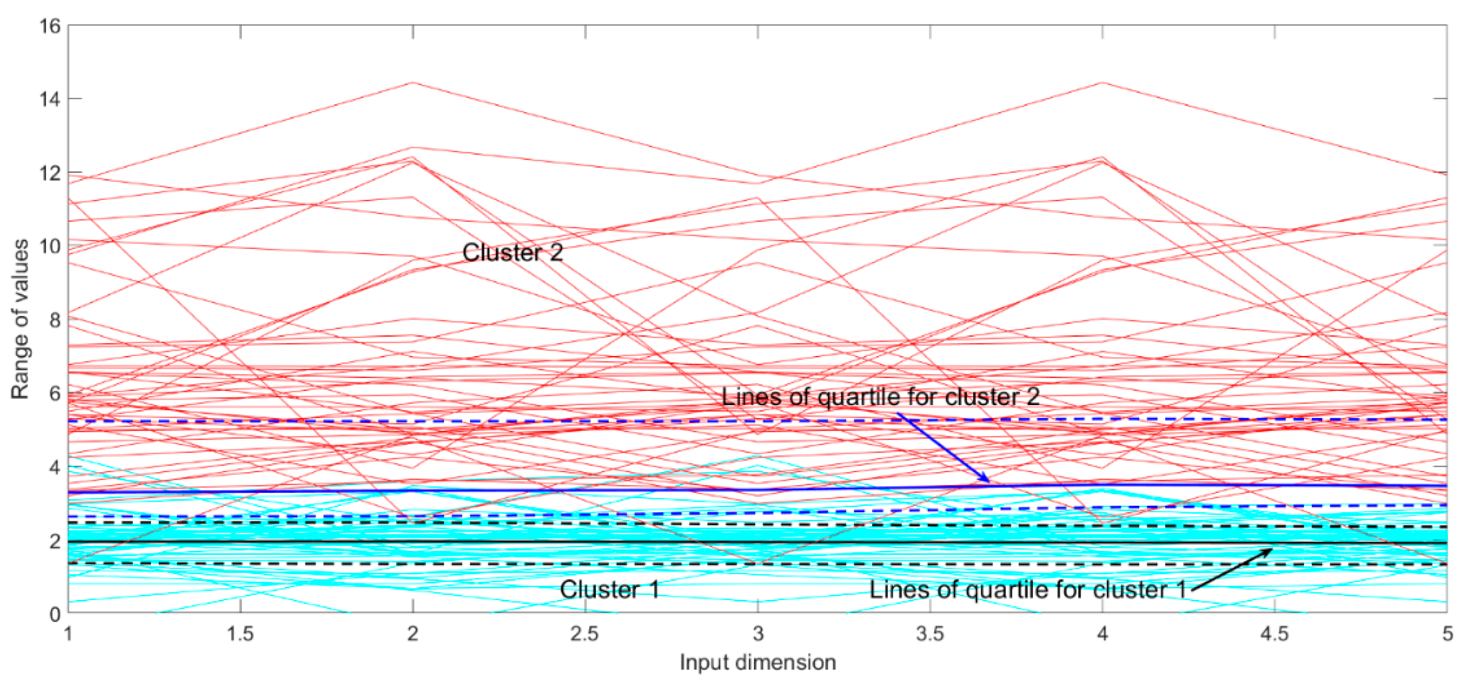
K-medoids, FCM and GMM methods, data points of the two clusters are 641|5659, 597|5703, 1082|5218 and 2066|4234, respectively. In contrast, though ADAP is time consuming, it has a better silhouette coefficient and data uniformity. Thus, the data by ADAP with two clusters is utilized for sequential research, shown in
Figure 9. Lines of quartile for each cluster clearly divide the data samples. It provides good foundation for establishment of a multi-model structure.
Taking WI as objective, a comparison of different data samples is shown in
Table 5 and
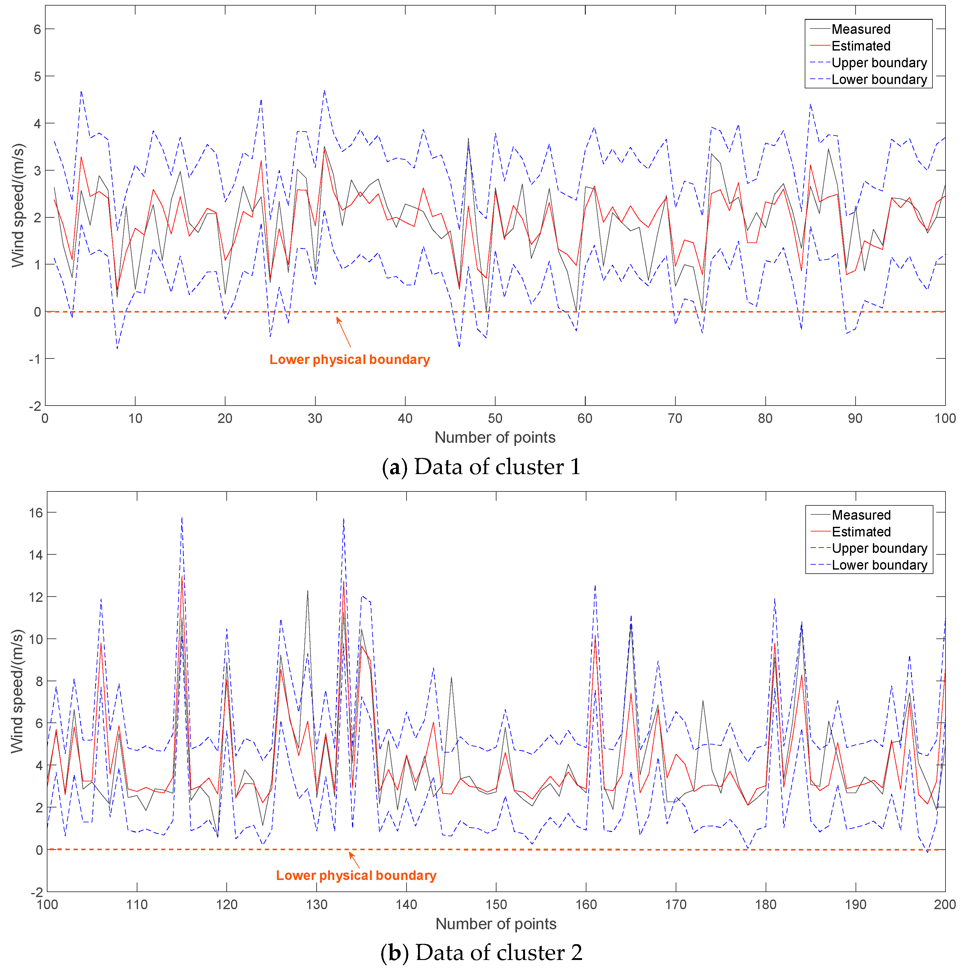
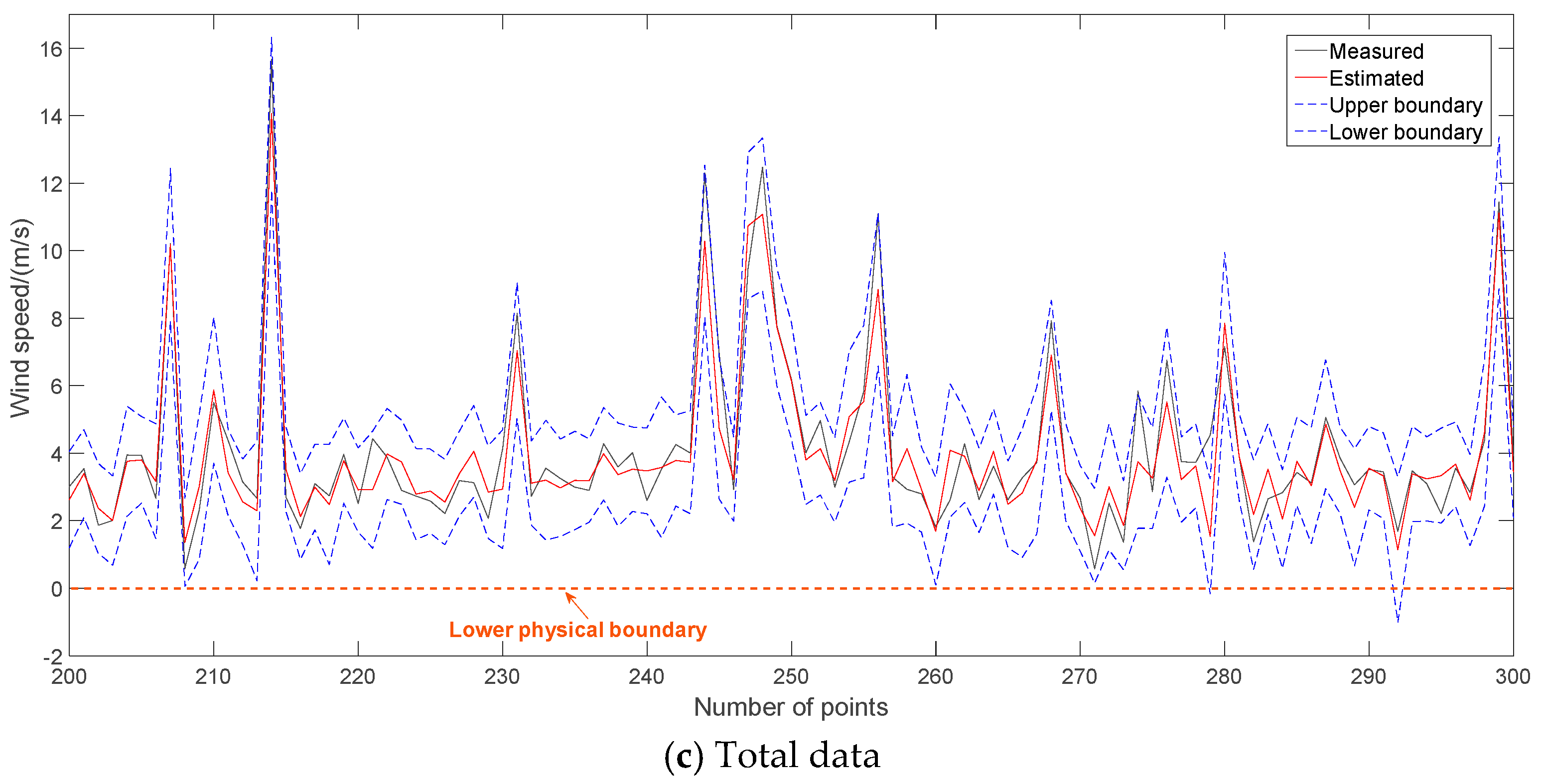
Figure 10, where five-fold cross validation is adopted to show the effectiveness of the GPR models. Analyzing the input data patterns in
Figure 9, the variation of the data of cluster-2 is stronger than that of the data of cluster-1. This explains, according to RMSE, NMACE and NPIAW, why he GPR model based on the data of cluster-2 performs worse than that based on the data of cluster-1. Due to the fact NRMSE is normalized by the mean value of output in Equation (19), it also explains that why the NRMSE values of cluster-2 are smaller than those of cluster-1. In contrast, the indexes of the GPR model based on total data samples are a compromise between that based on the data of cluster-1 and cluster-2.
The testing results suggest a truth, namely that that partition of wind speed patterns is uncertain to raise wind speed prediction accuracy for GPR modeling under a Bayesian framework. Regression and interval prediction by GPR is based on posterior probability of historical and new input data. It is highly dependent on distribution of the input data. In summary, for wind speed prediction by GPR, a multi-model structure doesn’t offer a significant improvement and its establishment may be unnecessary.
5.4. Wind Power Predcition Based on Single-Step Wind Speed Prediction Considering Sequential Uncertainties
Using the GPR model of single-step wind speed prediction in
Figure 10c and the new WTPC model, their sequential uncertainties for wind power prediction is studied in this subsection. Herein, 6377 data pairs of wind speed-power are adopted for WTPC modeling. As shown in
Figure 11, NRMSE, NMACE, NPIAW and WI of the final WTPC model via GPR are 0.2567, 0.007074, 0.2804 and 0.1813, respectively.
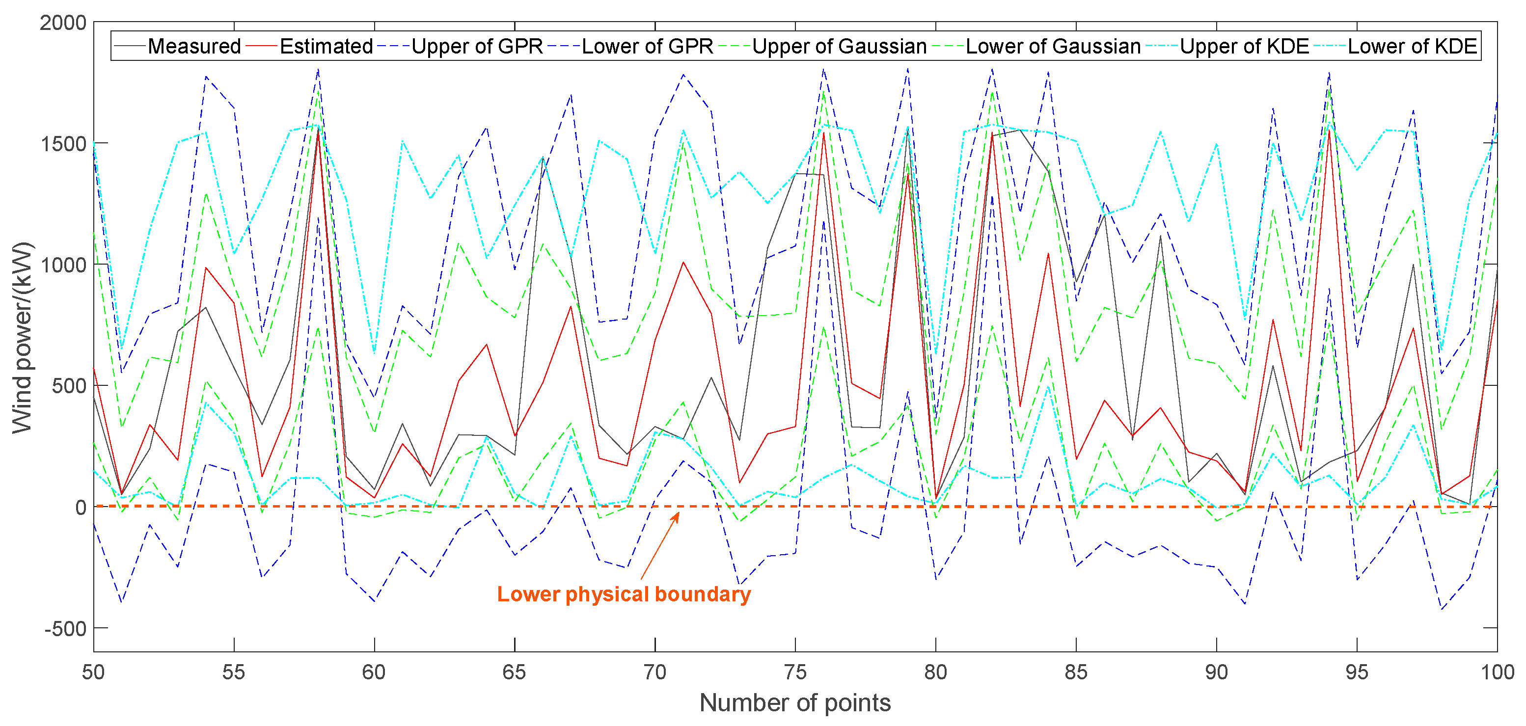
Considering the sequential uncertainties of wind speed prediction and WTPC modeling, the output of a single-step wind power prediction is shown in
Figure 12. Calculating the conditional probability distribution of the output error against the estimated power using the KDE and Gaussian methods, their confidence intervals under confidence 0.95 are also shown in
Figure 12. Gaussian is a parametric method for estimating confidence interval while KDE is a non-parametric method for that. Evaluation indexes for interval prediction performances, such as NMACE, NPIAW and WI, of them are shown in
Table 6. It can be found that the confidence interval of GPR is very similar with that of KDE and Gaussian. In
Figure 12, the upper and lower boundaries of these methods are directly shown from a statistical viewpoint to display the modeling effects while physical boundaries of wind power should be considered in actuality.
In summary, the above simulation results reflects a truth that the sequential uncertainties of wind speed prediction and WTPC modeling is perfectly validated. In the future, if a stepwise procedure is adopted for the wind power prediction of wind turbines, the accuracy of each step can be monitored and improved to guarantee a good final accuracy.
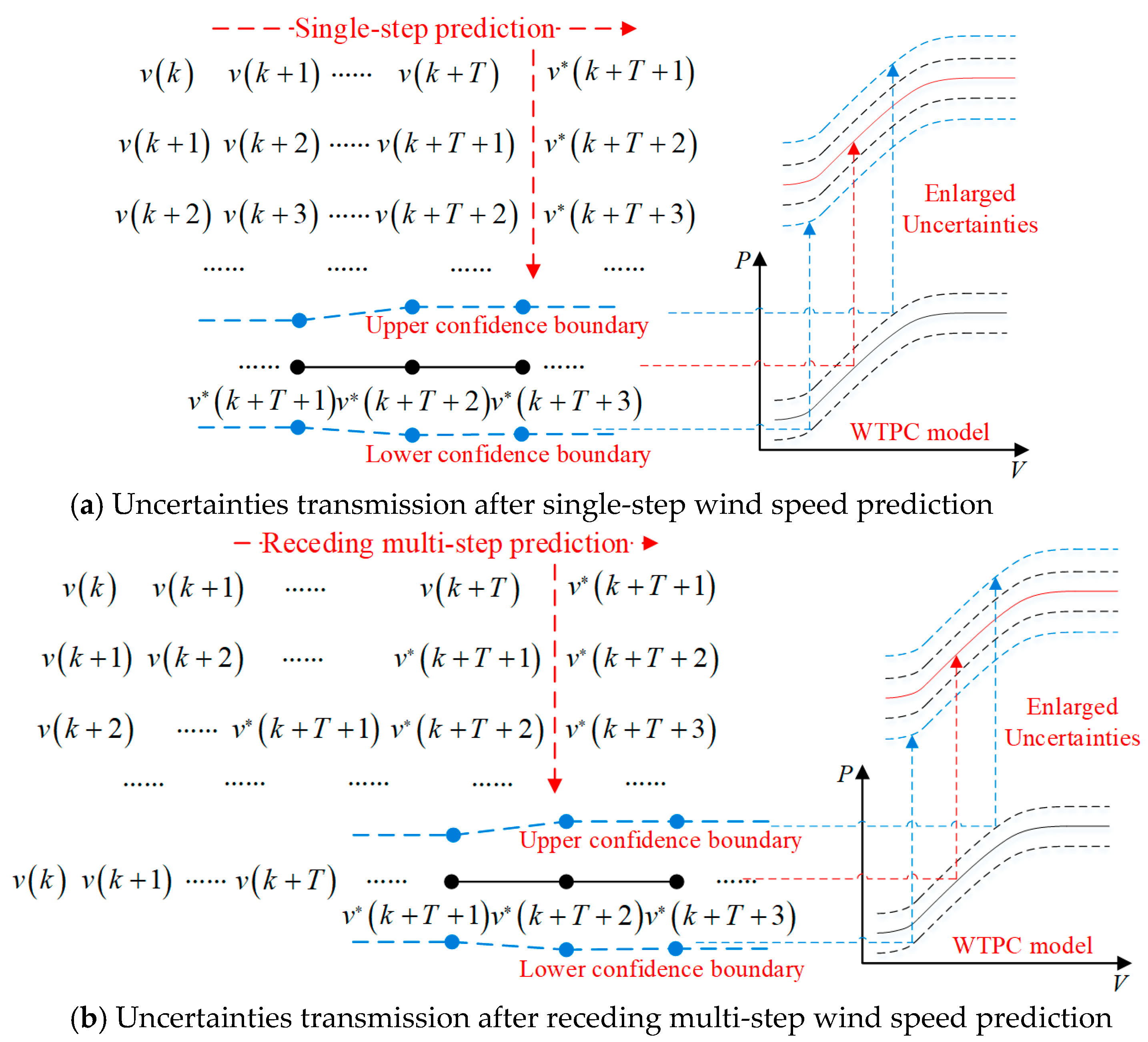
5.5. Wind Power Predcition Based on Multi-Step Wind Speed Prediction Considering Sequential Uncertainties
Different from the single-step prediction, multi-step wind speed prediction is discussed in this subsection. In this case, the uncertainties during multi-step prediction need to be considered. As introduced in
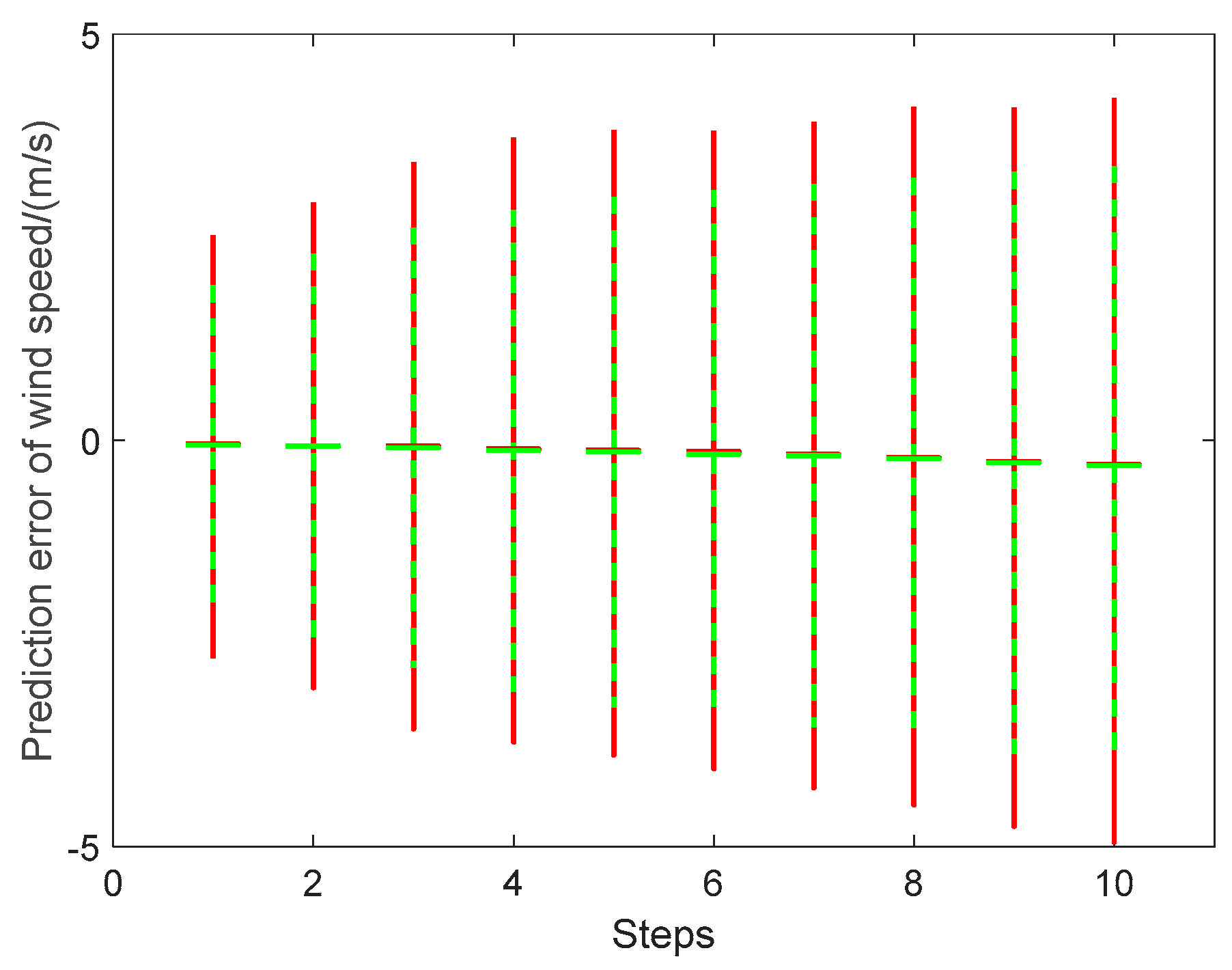
Section 3.3, only the statistics of the output error at each step are meaningful. Firstly, uncertainties transmission during ten-step wind speed prediction are shown in
Table 7 and
Figure 13, where the KDE and Gaussian methods are adopted to calculate the mean value and confidence intervals (with confidence 0.95) of the prediction error. All the statistical values of the KDE and Gaussian methods show the enlargement effects of receding steps during the ten-step wind speed prediction.
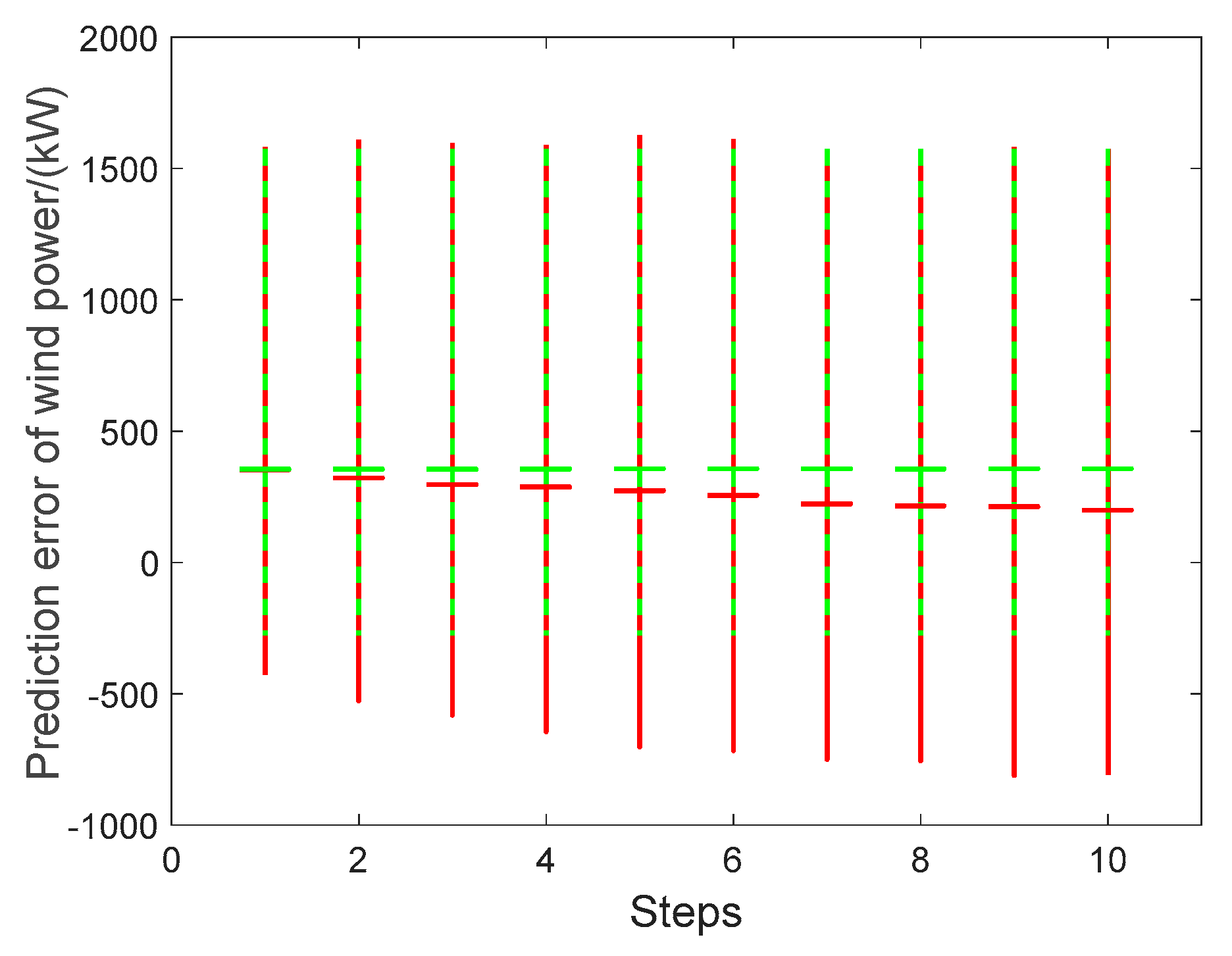
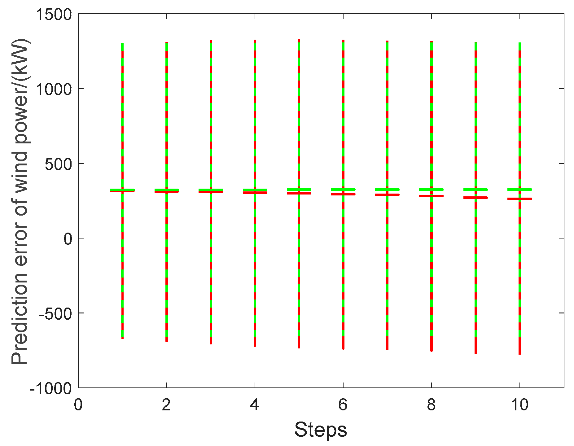
Using the actual wind speed or receding estimated wind speed as input, uncertainties transmission during ten-step wind power prediction are shown in
Table 8 and
Table 9,
Figure 14 and
Figure 15. For receding wind power using the actual wind speed as input, the input matrix is formed by one-step iteration. When it is input to the WTPC model, the outputs at different step are massively repetitive. As a result, when using the actual wind speed as input, the statistical values of the wind power error at each step remain relatively stable for both the KDE and Gaussian methods. In contrast, when using the receding estimated wind speed as input, the enlargement effects of receding steps during ten-step wind power prediction are significant. Especially, the upper and lower boundaries under confidence 0.95 show this enlargement effect. Mean values are calculated using positive and negative errors.
In summary, our simulation results clearly show the uncertainties transmission of receding ten-step wind power prediction from receding ten-step wind speed prediction, where the enlargement effects of receding steps also exist. In particular, wind power values of receding ten-step prediction using receding estimated wind speed as input have greater uncertainties than that using actual wind speed as input. Besides, a new uncertainty evaluation mechanism based on output error statistics is revealed here for receding multi-step predictions.
6. Conclusions
Wind speed and power prediction is a feasible and economic way to raise our knowledge of wind source and the controllability of wind power generation. Moreover, ultra-short-term wind power prediction is helpful to the refined operation of wind turbines and wind farms. Nowadays, this becomes more and more important. Considering the uncertainties of random factors, joint point-interval prediction of wind power via a Gaussian process regression (GPR) method is studied in this paper, where a stepwise procedure is adopted considering the sequential uncertainties of wind speed prediction and wind turbine power curve (WTPC) modeling. Testing via GPR, input-output matrix with five-dimensional input and one-dimensional output is determined for ultra-term wind speed prediction. On this basis, a principal component analysis (PCA)-adaptive affinity propagation (ADAP) scheme is validated to partition wind speed patterns with better silhouette coefficients and more uniform data clusters. Then, a multi-model structure for wind speed prediction can be built, but after validation it shows little improvement over single-model prediction via GPR. Subsequently, normalized evaluation indexes for joint point-interval estimation performance are defined. Through testing, a weighted-index (WI) must be used as objective for wind speed prediction by GPR while it is unnecessary for WTPC modeling by GPR, where a particle swarm optimization-differential evolution (PSO-DE) is adopted to guarantee optimization efficiency. Thereafter, the theoretical principle for the sequential uncertainties of wind speed prediction and WTPC modeling is deduced. Using kernel density estimation (KDE) and Gaussian methods to calculate confidence intervals of output error against estimated wind power, they are similar with that of GPR which perfectly validates the effectiveness of the uncertainties transmission principle. Besides, uncertainties transmission by stepwise procedure and uncertainties enlargement by receding steps are also revealed where a new evaluation mechanism based on statistics to output error is revealed using KDE and Gaussian methods. Overall, the above research should prove meaningful for uncertainty prediction of wind power in the ultra-short-term and is very helpful for the future development of wind power generation.


