Abstract
Low-field nuclear magnetic resonance (NMR) has been widely used in the petroleum industry for reservoir evaluation. Fluid properties and petrophysical parameters can be determined from NMR spectra, obtained from processing echo data measured from the NMR tool. The more accurate NMR spectra are, the higher the reliability of reservoir evaluation based on NMR logging is. The purpose of this paper is to obtain more precise T1–T2 spectra in heavy oil reservoirs, with focus on the T1–T2 data acquisition and inversion. To this end, four inversion algorithms were tested on synthetic T1–T2 data, their precision was evaluated and the optimal inversion algorithm was selected. Then, the sensitivity to various acquisition parameters (wait time and echo spacing) was evaluated with T1–T2 experiments using a disordered accumulation of glass beads with a diameter of 45 μm saturated with heavy oil and distilled water. Finally, the sensitivity to various inversion parameters (convergence tolerance, maximum number of iterations and regularization parameter) was evaluated using the optimal inversion algorithm. The results showed that the inverted T1–T2 spectra loss some relaxation information when the number of echo train is less than 7. The peak of the heavy oil signal gradually moves along the direction of increase in the T2 and the intensity of the heavy oil signal gradually decreases with increasing echo spacing. The echo spacing should be as small as possible for T1–T2 measurements in heavy oil reservoirs on the premise that the NMR instrument operates normally. A convergence tolerance that is too large or a maximum number of iterations that is too small may result in exiting the iteration prematurely during the inversion. A convergence tolerance of 1 × 10⁻⁷ and a maximum number of iterations of 30,000 are recommended for the inversion of the T1–T2 spectra. An appropriate regularization parameter is an important factor for obtaining accurate T1–T2 spectra from the optimal inversion algorithm.
1. Introduction
Heavy oil is characterized by a high viscosity of more than 100 cp and low American Petroleum Institute (API) gravity in the range of 10–20°. Worldwide heavy oil reserves are about 6 trillion barrels [1,2,3,4]. Due to the decrease in conventional oil and gas production, an increasing number of researchers have focused on the exploration and development of heavy oil reservoirs. The nuclear magnetic resonance (NMR) technique can be used to evaluate the viscosity and components of crude oil and provides an effective and economical method for evaluating wells; therefore, it has been widely used in reservoir exploration [5,6,7,8,9]. In recent years, several researchers have studied the NMR properties of heavy oil samples and the NMR responses of heavy oil reservoirs; these studies have advanced the application of NMR techniques in heavy oil reservoirs. Kleinberg and Vinegar (1996) used NMR experiments and discovered that heavy oil is characterized by a lower apparent hydrogen index at an API gravity <17° [10]. Freedman et al. (1997) determined that oil with a viscosity of less than 1000 cp varies inversely with the transverse relaxation time (T2) [11]. LaTorraca et al. (1999) studied the T2 spectra of heavy oil samples with different echo spacings and concluded that the amplitude of the T2 spectra gradually decreased and the peak moved in the direction of the T2 increase as the echo spacing increased [6]. Mirotchnik et al. (1999) identified bitumen in heavy oil based on one-dimensional (1D) NMR logging and believed that the signal of heavy oil might be partially lost during NMR measurements [12]. Wayne and Doug (1999) detected heavy oil on the North Slope Satellite Fields of Alaska based on NMR logging and found out that the NMR porosity was lower than the actual porosity in heavy oil reservoirs [13]. Galford and Marschall (2000) estimated the information of movable water in heavy oil reservoirs using an enhanced diffusion method and evaluated heavy oil reservoirs through conventional and NMR logging [1]. Sun et al. (2006) and Chen et al. (2006) proposed a Poroperm + Heavy Oil sequence for NMR diffusion–relaxation time (D–T2) measurements in heavy oil fields in Venezuela and Kazakhstan [14,15]; the movable water, bound water, heavy oil and effective porosity can be determined reliably based on the D–T2 spectra but unfortunately the authors did not report the measurement parameters. Liu et al. (2013) measured the three-dimensional (3D) NMR responses of three heavy oil samples at a magnetic field gradient of 23.55 T/m using a unilateral NMR instrument with a Larmor frequency of 20 MHz and analyzed the components and internal properties of the heavy oil samples [3]. Their findings showed that the ratio of the longitudinal relaxation time to the transverse relaxation time (T1/T2) was low for the light components and high for the heavy components of the heavy oil samples. Enninful et al. (2017) determined the flexible cut-off value between water and heavy oil based on the local minima of T2 spectra and then combined the determined flexible cut-off and a fixed cut-off of the T1/T2 ratio to evaluate heavy oil based on the T1–T2 spectra [16].
The irreducible water and heavy oil signals may overlap in the T2 spectra due to their similar transverse relaxation time, resulting in the unreliable of T2-based heavy oil reservoir evaluation. Two-dimensional (2D) NMR can measure simultaneously two kinds of relaxation information and it can be used for distinguishing the irreducible water and heavy oil due to their different diffusion coefficients and T1/T2. As a result, 2D NMR is very important in the evaluation of heavy oil reservoirs. Past publications on NMR-based heavy oils study also indicate that 2D NMR techniques have become increasingly popular for the evaluation of heavy oil reservoirs. There is a non-convergence phenomenon for the heavy oil signal in D–T2 spectra, thus a quantitative evaluation of heavy oil reservoirs is difficult based on D–T2 spectra. Fortunately, T1/T2 is higher for heavy oil than for water and the heavy oil signals are convergent in the T1–T2 spectra. Therefore, T1–T2 spectra are the mainstream method to evaluate heavy oil reservoirs. To date there are no publications that report the T1–T2 measurement parameters in the heavy oil reservoirs. Indeed, the precision of T1–T2 spectra is seriously affected by measurement parameters. To optimize T1–T2 spectra of heavy oil reservoirs, the determination of the acquisition parameters is very necessary.
The inversion of NMR T1–T2 spectra is a seriously ill-posed problem. Thus, employing an accurate and efficient inversion method is a precondition and a base for the investigation of the T1–T2 spectra of heavy oil reservoirs. To date, many inversion methods have been developed, including the truncated singular value decomposition (TSVD) method [17,18,19,20], the single-parameter regularization method [21,22,23,24,25,26,27,28], the double-parameter regularization method [29,30], the Monte Carlo method [31,32,33] and some other methods. Even if a robust inversion method is employed, the ideal T1–T2 spectra cannot be obtained if the inversion parameters are inappropriate. Therefore, the determination of the inversion parameters for the T1–T2 spectra of heavy oil reservoirs is also of great significance to obtain accurate T1–T2 spectra.
2. Basic Theory of T1–T2 Spectra
The pulse sequences used for NMR T1–T2 measurements mainly include: (1) inversion recovery-Carr–Purcell–Meiboom–Gill (IR-CPMG) and (2) saturation recovery-CPMG (SR-CPMG), diagrams of which are shown in Figure 1 [23,34]. A major difference between the two is the T1-editing phase. The dynamic range of the measured magnetization using the first pulse sequence is from −M0 to M0, whereas the dynamic range of the measured magnetization using the second pulse sequence is from 0 to M0. The first pulse sequence has the advantage of a wider measured magnetization range and a higher resolution for a shorter T1 component. Due to the shorter relaxation time of heavy oil, the IR-CPMG pulse sequence was chosen to study the influencing factors of the T1–T2 spectra in heavy oil reservoirs.
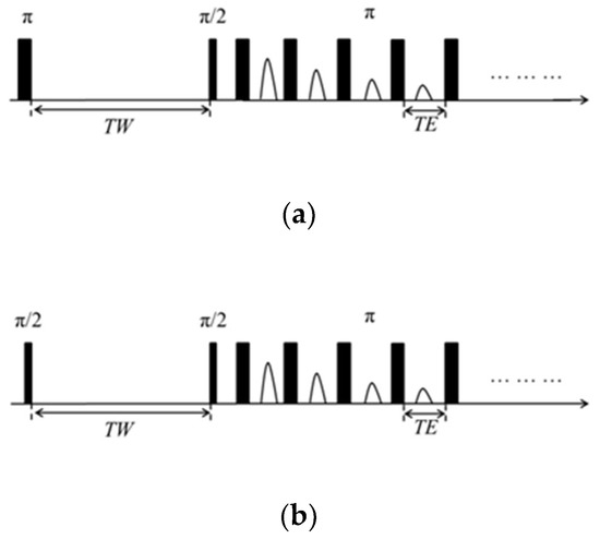
Figure 1.
Diagrams of the inversion recovery-Carr–Purcell–Meiboom–Gill (IR-CPMG) pulse sequence (a) and the saturation recovery Carr-Purcell-Meiboom-Gill (SR-CPMG) pulse sequence (b).
The measured echo data using the IR-CPMG pulse sequence can be written based on the Fredholm integral equation of the first kind:
where t is the measuring time; are the measured echo data with a wait time of TW at time t; is the unknown T1–T2 spectra to solve; is the noise.
The discrete form of Equation (1) can be expressed as:
where and are the measured echo data and noise with the mth (m = 1, 2, 3, … M) wait time at time ti (i = 1, 2, 3, … I); is the amplitude in the unknown T1–T2 spectra to solve.
The matrix form of Equation (2) is written as:
where Y and E with a size of K × I are the measured echo data and noise; the elements of K1 with a size of M × P are ; the elements of K2 with a size of I × J are ; S with a size of P × J is the unknown T1–T2 spectra to solve; superscript T represents the transpose of the matrix.
The 2D NMR spectra inversion problem can be described as a problem of how to solve S under the condition that the measured data Y and the kernel matrices K1 and K2 are known. In a 2D NMR spectra inversion problem, 2D problem is usually transformed to a 1D problem, which is then solved using an inversion algorithm; subsequently, the 1D solution is reallocated to a 2D space. Thus, we can obtain
where ; ; ; vect() denotes the operator creating a vector by stacking all the columns of a matrix; ; denotes the Kronecker product of two matrices.
Equation (4) can be replaced by the least squares fitting problem as:
Because the matrix K is ill-conditioned, the solution of Equation (5) is unsteady and affected seriously by noise. Usually, the regularization method is used to suppress the noise. The regularization method adds a penalty term to the Equation (5) and adjusts the regularization parameter to seek a trade-off between the solution accuracy and the noise sensitivity. The objective function for the regularization method can be written as:
where is the regularization parameter that controls the weight of the residual and the regularization term; is the penalty function. Different regularization methods have different penalty functions; for example, for an L2 regularization method, for an L1 regularization method and for a maximum entropy regularization method. The penalty function consists of two kinds of functions for a double-parameter regularization method. The different penalty functions constrain the different properties of the objective function’s solution. We summarized some inversion methods for the inversion problem in Appendix A, Appendix B and Appendix C.
3. Numerical Simulation and Inversion Algorithm Selection
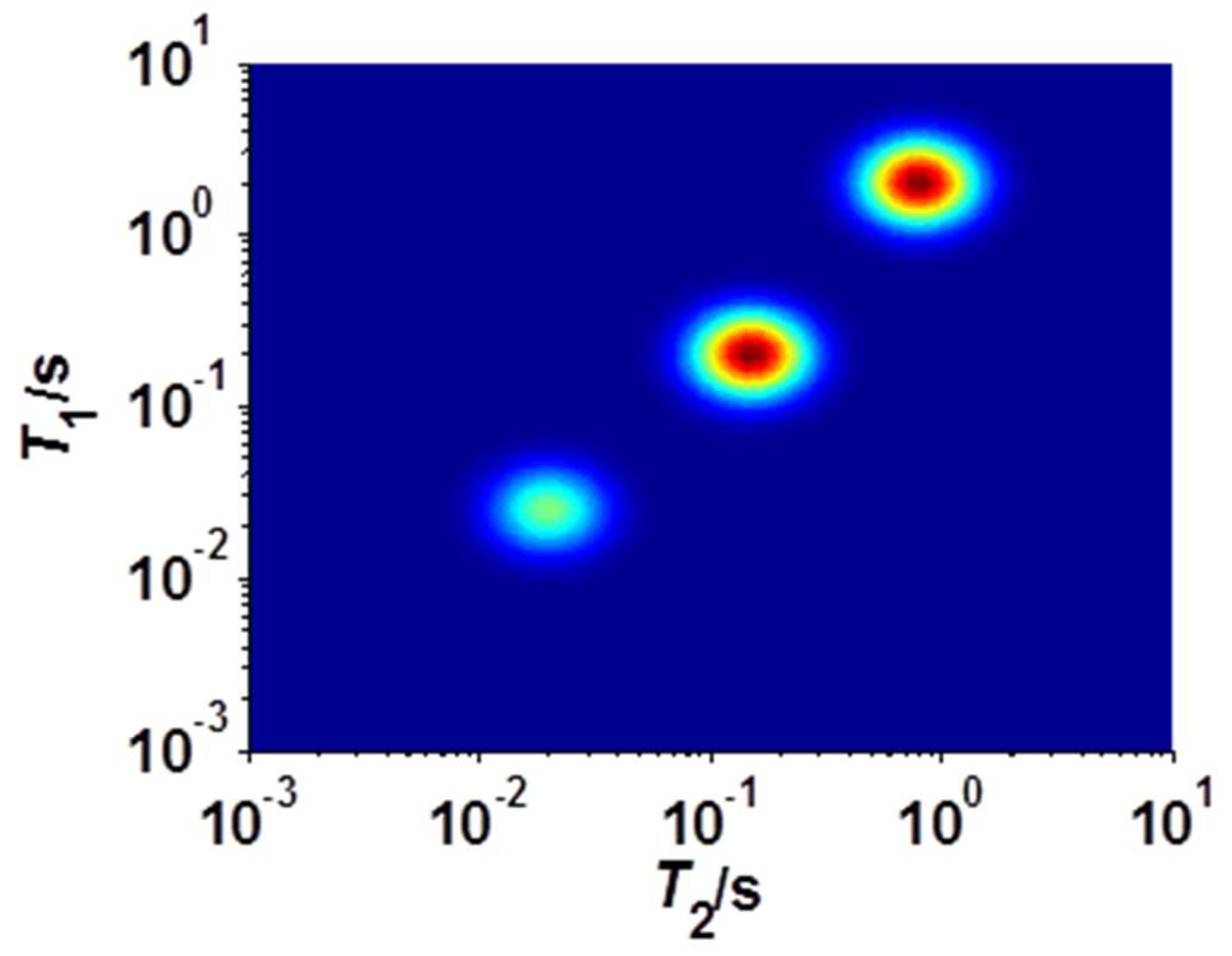
The effectiveness of the mentioned algorithms in the appendices for low signal-to-noise ratio (SNR) data was evaluated from numerical simulation. A T1–T2 spectra model (Figure 2) was constructed and it contains oil, free water and bound water, the porosities of which are 6 pu, 6 pu and 3 pu and the T1, T2 values of which are 2.0 s, 0.8 s and 0.2 s, 0.15 s and 0.025 s, 0.02 s. The following forward parameters were set: the echo spacing is 0.2 ms; echo number is 4000; the wait time group is [0.001 0.003 0.01 0.03 0.1 0.3 1.0 3.0 6.0 9.0 12.0 15.0 18.0 21.0 24.0] s. The echo data with different wait times according to Equation (2) were calculated and Gaussian noises with different SNRs (50, 20 and 10) were added to the calculated echo data. To improve the inversion speed, the calculated noisy echo data number was compressed to 200 using the fast SVD (FSVD) method [35,36]. Subsequently, the compressed echo data were inverted using the two-step iterative shrinkage/thresholding (TIST) algorithm, the TSVD algorithm, the Butler-Reeds-Dawson (BRD) algorithm and the Levenberg-Marquardt (LM) algorithm to obtain the corresponding T1–T2 spectra, as shown in Figure 3, Figure 4 and Figure 5.

Figure 2.
T1–T2 spectra model.

Figure 3.
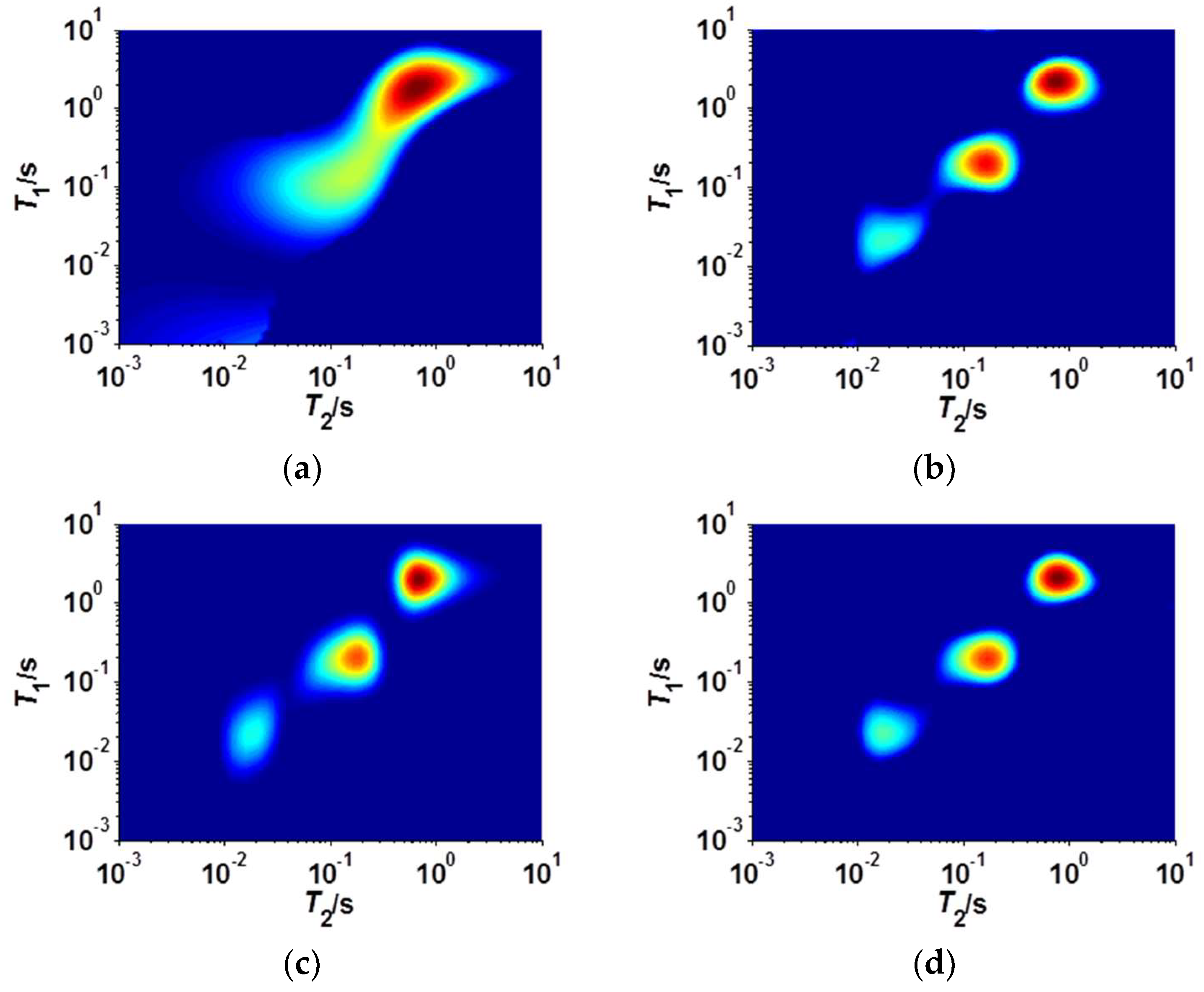
Comparison of the inverted T1–T2 spectra obtained from the four algorithms at SNR = 50. (a–d) represent the results of the truncated singular value decomposition (TSVD), Butler-Reeds-Dawson (BRD), Levenberg-Marquardt (LM) and two-step iterative shrinkage thresholding (TIST) algorithms, respectively.
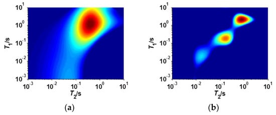
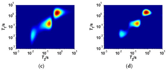
Figure 4.
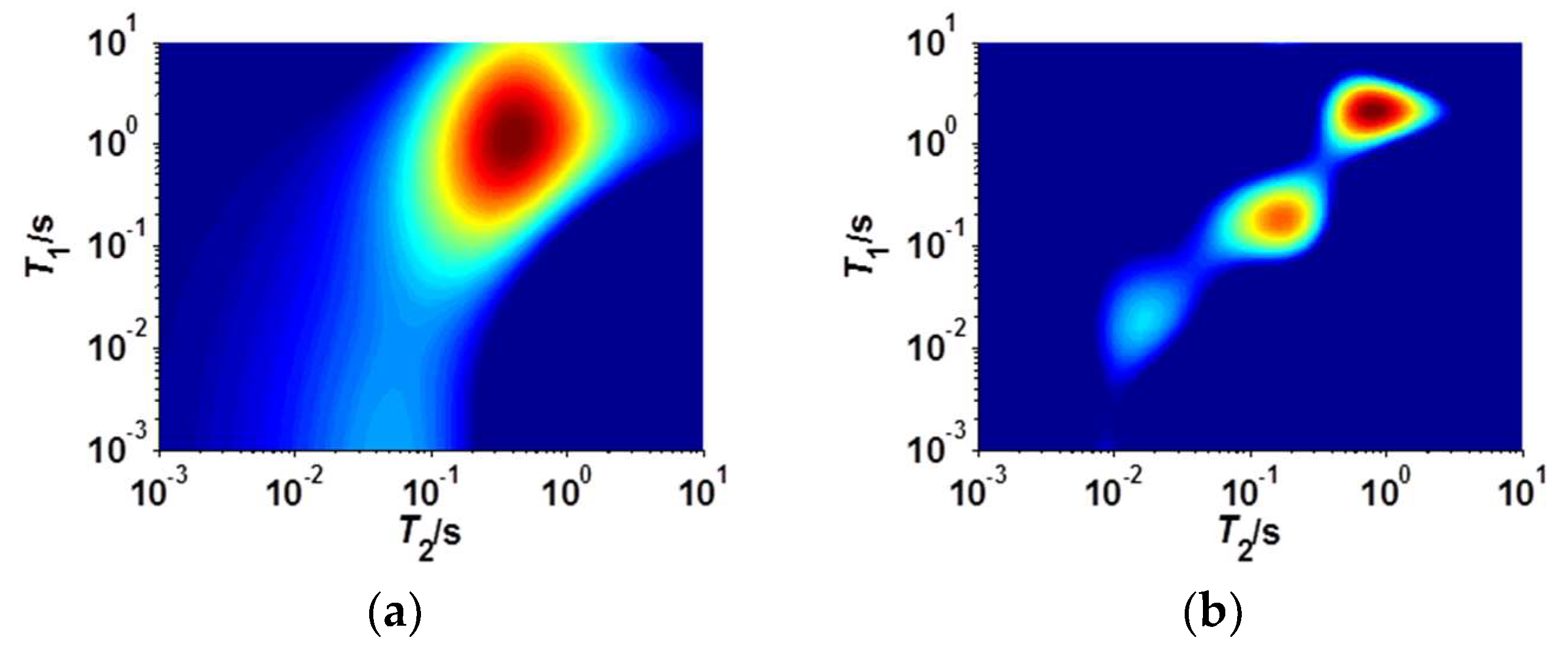
Comparison of the inverted T1–T2 spectra obtained from the four algorithms at SNR = 20. (a–d) represent the results of the TSVD, BRD, LM and TIST algorithms, respectively.

Figure 5.
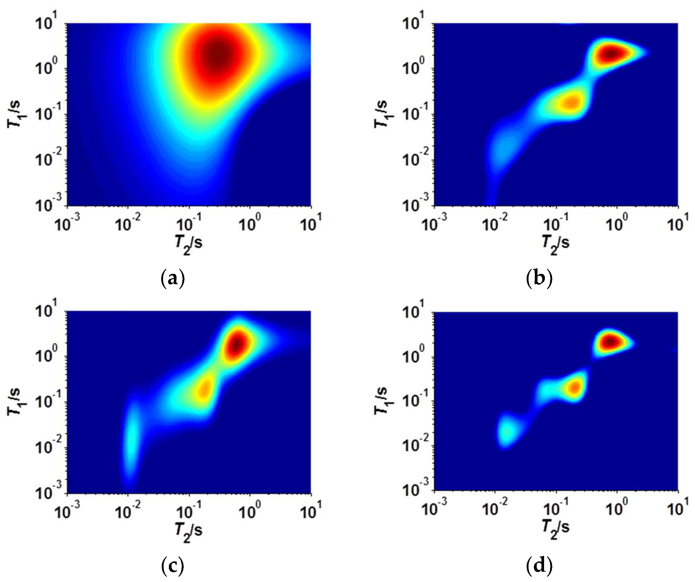
Comparison of the inverted T1–T2 spectra obtained from the four algorithms at SNR = 10. (a–d) represent the results of the TSVD, BRD, LM and TIST algorithms, respectively.
The inverted T1–T2 spectra obtained from the TSVD algorithm are different from the model at an SNR of less than 50 and the oil, free water and bound water signals overlap; moreover, the bound water signal may disappear in the inverted T1–T2 spectra. As the SNR decreases, the signals of the oil, free water and bound water gradually diverge in the inverted T1–T2 spectra obtained from the BRD algorithm and the LM algorithm and the ability to identify the fluids based on the inverted T1–T2 spectra gradually decreases. The inverted T1–T2 spectra obtained from the TIST algorithm clearly show the signals of oil, free water and bound water and the signal divergence degrees are lower than those of the BRD algorithm and the LM algorithm. Above all, the TIST algorithm possesses stronger robustness for the NMR T1–T2 data inversion than the other inversion algorithms. Moreover, we compared the detailed results of the four-inversion algorithm, as described in Table 1. It is evident that the calculated porosity of the inverted T1–T2 spectra from the TIST algorithm is closest to the model’s porosity and the relative error and residual of the TIST algorithm are lower than for the other inversion algorithms under the condition of the same SNR. With the decrease in the SNR, the relative error of the TIST algorithm gradually decreases but its rate of decrease is smaller than that of the others. Judging from these results, the TIST algorithm is superior to the TSVD algorithm, the BRD algorithm and the LM algorithm for inverting NMR T1–T2 data with a low SNR. Therefore, the TIST algorithm was recommended for NMR data inversion in heavy oil reservoirs.

Table 1.
Comparison of detailed results of the four algorithms with different SNRs.
4. Parameter Analysis of T1–T2 Spectra in Heavy Oil Reservoirs
After selecting the optimal inversion algorithm, NMR experiments were implemented to study the T1–T2 spectra characteristics of heavy oil with different acquisition and inversion parameters, whose aim is to obtain the optimal T1–T2 spectra of heavy oil reservoirs. Due to the production difficulty of heavy oil-saturated underground rock, a disordered accumulation of glass beads with a diameter of 45 μm saturated with about 1500 cp heavy oil and distilled water was selected as the experimental sample. Firstly, the glass beads were put in a glass vial and then 1.5 grams of distilled water and 3.0 grams of heavy oil from oilfields were added in the glass vial. Next, the glass vial was sealed up and heated in a water bath until the fluids were completely saturated in the pore. Finally, the glass vial was taken out and dropped to room temperature. When the experimental sample was prepared well, it would be put in the NMR instrument. Input the T1–T2 measurement parameters and start NMR experiments. All the NMR experiments were done using a 2 MHz NMR Rock Core Analyzer produced by Magritek under room temperature.
4.1. Acquisition Parameters
In this study, the IR-CPMG pulse sequence was chosen to study the T1–T2 spectra in NMR experiments. The acquisition parameters mainly include the wait time group and echo spacing during the T1–T2 measurements. Therefore, different wait time groups and echo spacings were set and used in NMR T1–T2 experiments for a disordered accumulation of glass beads and then the measured echo data were processed to obtain the corresponding T1–T2 spectra. The purpose was to find the optimal wait time group and echo spacing for the T1–T2 spectra of heavy oil reservoirs.
4.1.1. Wait Time Group
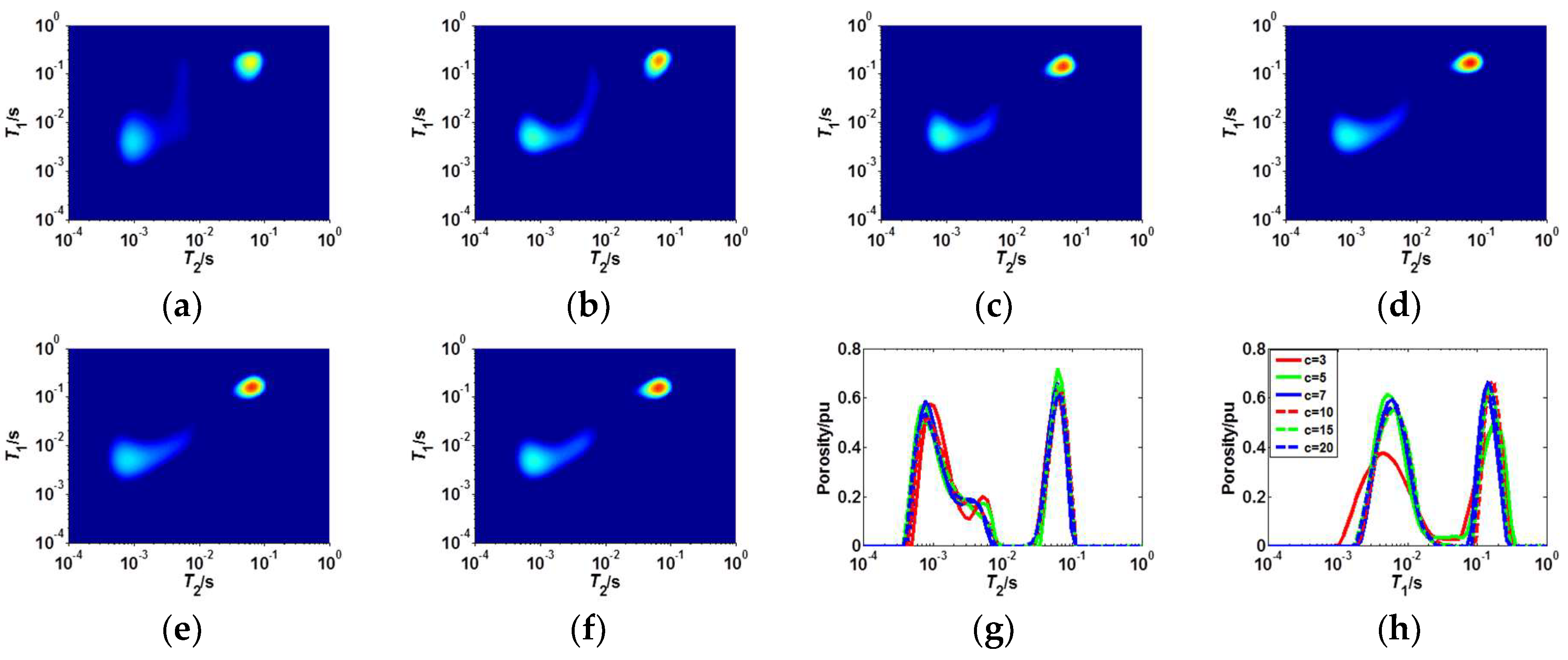
To find the optimal wait time group for the T1–T2 spectra of heavy oil reservoirs, the echo spacing and echo number were fixed and the only wait time group was changed in NMR T1–T2 experiments. The maximum and minimum wait time were set to 1 s and 0.0001 s based on the properties of heavy oil and water. Six wait time groups were set and listed in Table 2 and the echo spacing and echo number were set to 0.15 ms and 2000, respectively. A major difference among the six wait time groups is the number of echo train. After the experiments, the corresponding echo data with the six wait time groups were acquired. Subsequently, the corresponding T1–T2 spectra were obtained using the TIST algorithm after the number of echo data was compressed to 200 by the FSVD method, as shown in Figure 6a–f. Figure 6g,h show the T2 and T1 spectra from the T1–T2 spectra projections onto the T1 and T2 axes, respectively.

Table 2.
Wait time group.

Figure 6.
Inverted T1–T2 spectra, T1 spectra and T2 spectra in heavy oil reservoirs for different wait time groups. (a–f) represent the inverted T1–T2 spectra for the first to sixth wait time groups, respectively. (g,h) represent the T2 and T1 spectra from the T1–T2 spectra projections onto the T2 and T1 axes, respectively.
The water signal is partially lost when the number of echo train in the wait time group is no more than 5 and the heavy oil signal is partially lost when the number of echo train is 3, indicating that too few number of echo train in the wait time group are undesirable for T1–T2 measurements in heavy oil reservoirs. The inverted T1–T2 spectra are the same for the third to sixth wait time group, which indicates that increasing the number of echo train in the wait time group has no effect on the inverted T1–T2 spectra when the number of echo train is up to 7. It should be noted that increasing the number of echo train just increases the T1–T2 measurement time and the computation time of the inversion. Above all, the quality of the T1–T2 spectra in heavy oil reservoirs depends on the number of echo train when the maximum and minimum wait time were fixed and the number no less than 7 is appropriate. Considering all factors, the third wait time group is more suitable than the other five wait time groups for T1–T2 measurements in heavy oil reservoirs. It can be seen from Figure 7g,h that the inverted T1 spectra are strongly affected by the wait time group but the inverted T2 spectra with different wait time groups are the same. Therefore, in the event that an inappropriate wait time group is used for the T1–T2 measurement in heavy oil reservoirs, the projected T2 spectra can still be used for reservoir evaluation.

Figure 7.
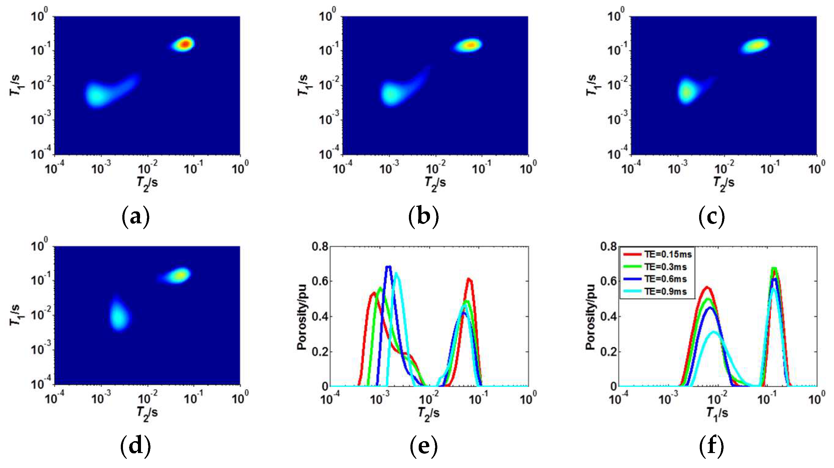
Inverted T1–T2 spectra, T1 spectra and T2 spectra in heavy oil reservoirs for different echo spacings. (a–d) represent the inverted T1–T2 spectra with echo spacings of 0.15 ms, 0.3 ms, 0.6 ms and 0.9 ms, respectively. (e,f) represent the T2 and T1 spectra from the T1–T2 spectra projections onto the T2 and T1 axes, respectively.
4.1.2. Echo Spacing TE
To find the optimal echo spacing for the T1–T2 spectra of heavy oil reservoirs, the wait time group was fixed and the echo spacing was changed, the values of which were 0.15 ms, 0.3 ms, 0.6 ms and 0.9 ms. The echo number was set to int (300 ms/TE) and the sixth wait time group in Table 2 was used. After the experiments, the corresponding echo data with different echo spacings were acquired. Subsequently, the corresponding T1–T2 spectra were obtained using the TIST algorithm after the number of echo data was compressed to 200 by the FSVD method, as shown in Figure 7a–d. Figure 7e,f represent the T2 and T1 spectra from the T1–T2 spectra projections onto the T2 and T1 axes, respectively.
Figure 7 showed that the peak of the heavy oil signal gradually moves along the direction of increase in T2 and the intensity of the heavy oil signal gradually decreases as the echo spacing increases in the inverted T1–T2 spectra. The water signal changed slightly in the inverted T1–T2 spectra when the echo spacing is in the range of 0.15 ms to 0.9 ms. This occurs because the T2 of the water is two order of magnitude longer than that of heavy oil and as the echo spacing increases, the heavy oil signal begins to disappear due to attenuation before acquiring the signal at the first time but the water signal does not disappear in the time of one echo spacing. Therefore, the echo spacing should be as small as possible for T1–T2 measurements in heavy oil reservoirs on the premise that the NMR instrument operates normally; this reduces the loss of the heavy oil signal and improves the accuracy of the reservoir evaluation.
4.2. Inversion Parameters
For echo data with a high SNR and appropriate acquisition parameters, the inverted T1–T2 spectra may be inaccurate if the inversion parameters are not chosen appropriately. In other words, the inversion result is sensitive to the inversion parameters. T1–T2 experimental data with fixed wait time group and echo spacing as an example to find the optimal inversion parameters on the T1–T2 spectra of heavy oil reservoirs. The acquisition parameters of the T1–T2 measurements were fixed as follows: the echo spacing was 0.15 ms; the echo number was 2000; the sixth wait time group in Table 2 was used. Subsequently, the number of measured echo data was compressed to 200 and the compressed echo data were inverted using the TIST algorithm with different inversion parameters to obtain the corresponding T1–T2 spectra. The inverted T1–T2 spectra with different inversion parameters, including the convergence tolerance tol, the maximum number of iterations itermax and the regularization parameter, were compared to choose the optimal inversion parameters.
4.2.1. Convergence Tolerance tol
An appropriate convergence tolerance tol is helpful not only to obtain accurate T1–T2 spectra but also to improve the inversion efficiency. A convergence tolerance that is too large may result in exiting the iteration prematurely during the inversion and the inversion results might be inaccurate. A convergence tolerance that is too small may result in redundant iterations during the inversion, resulting in time-consuming inversion process. Six different convergence tolerances were set: 1 × 10⁻⁹, 1 × 10⁻⁸, 1 × 10⁻⁷, 1 × 10⁻⁶, 1 × 10⁻⁵ and 1 × 10⁻⁴. Then, the compressed echo data were inverted using the TIST algorithm with different convergence tolerances to obtain the corresponding T1–T2 spectra, as shown in Figure 8a–f. Figure 8g,h show that the T2 and T1 spectra from the T1–T2 spectra projections onto the T2 and T1 axes, respectively. It can be observed from the inverted T1–T2 spectra that the heavy oil signal and the water signal have an obvious divergence when the convergence tolerance tol is no less than 1 × 10⁻⁶. It can be seen from the projected T1 spectra and T2 spectra that decreasing the convergence tolerance has no effect on the inversion results when the convergence tolerance is no more than 1 × 10⁻⁷; when the convergence tolerance tol is more than 1 × 10⁻⁷, the amplitudes of the heavy oil signal and the water signal decrease gradually with increase of convergence tolerance. The reason is that the iteration stops prematurely in the TIST algorithm and the solution has not absolute convergence when the convergence tolerance is larger. To sum up, a convergence tolerance tol of 1 × 10⁻⁷ was recommended for T1–T2 spectra inversion of heavy oil reservoirs.
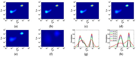
Figure 8.
Inverted T1–T2 spectra, T1 spectra and T2 spectra in heavy oil reservoirs with different convergence tolerances. (a–f) represent the inverted T1–T2 spectra with convergence tolerances of 1 × 10⁻⁹, 1 × 10⁻⁸, 1 × 10⁻⁷, 1 × 10⁻⁶, 1 × 10⁻⁵ and 1 × 10⁻⁴, respectively. (g,h) represent the T2 and T1 spectra from the T1–T2 spectra projections onto the T2 and T1 axes, respectively.
4.2.2. Maximum Number of Iterations itermax
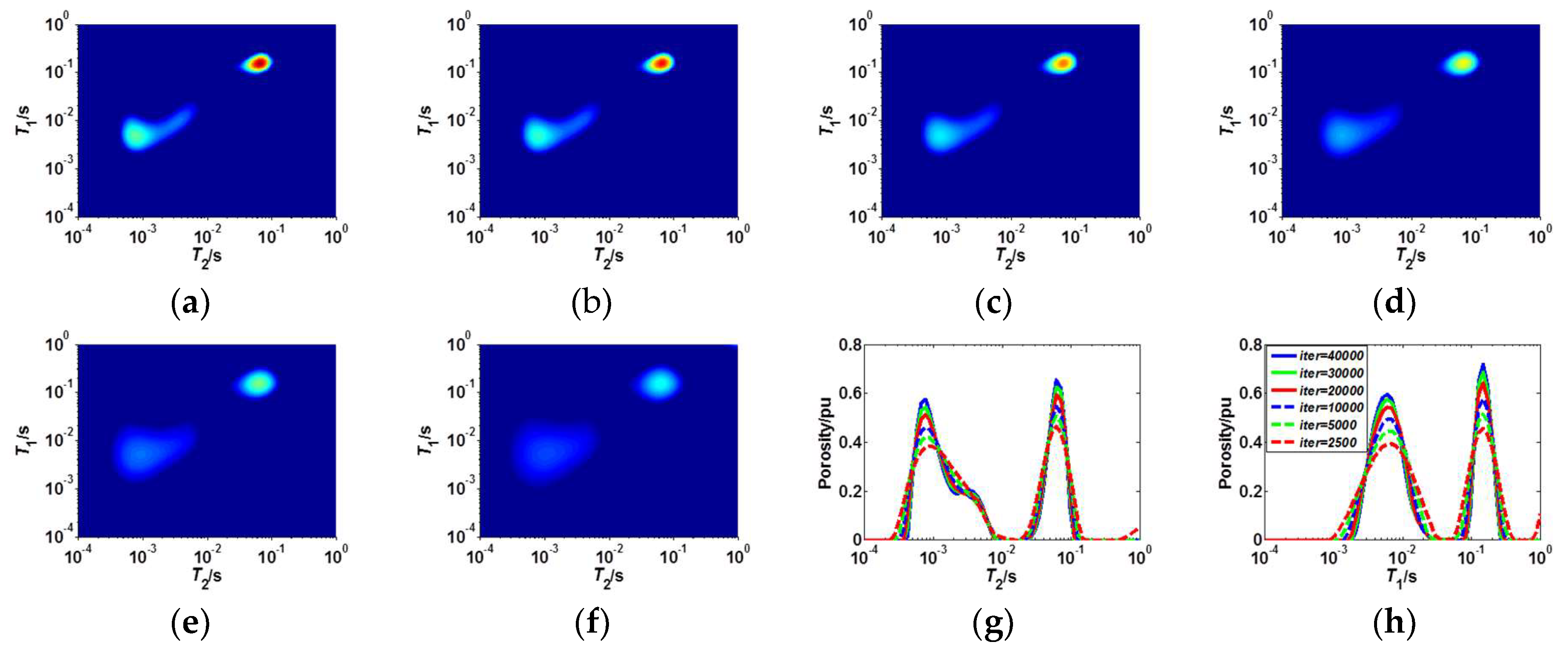
Similar to the convergence tolerance effect, the maximum number of iterations itermax also affects the inversion efficiency. A maximum number of iterations that is too large may result in redundant iterations during the inversion, resulting in time-consuming inversion process. Six different maximum numbers of iterations were set: 40,000, 30,000, 20,000, 10,000, 5000 and 2500. Then, the compressed echo data were inverted using the TIST algorithm with the six maximum numbers of iterations to obtain the corresponding T1–T2 spectra, as shown in Figure 9a–f. Figure 9g,h show the T2 and T1 spectra from T1–T2 spectra projections onto the T2 and T1 axes, respectively. It was evident that the heavy oil signal and the bound water signal gradually diverge in the inverted T1–T2 spectra and their amplitudes gradually decrease with a decrease in the maximum number of iterations. Increasing the maximum number of iterations has no obvious effect on the inversion results when the maximum number of iterations is up to 30,000; the amplitudes of the heavy oil signal and the water signal increase gradually with increase of convergence tolerance. This occurs because the accuracy of the solution is very low for the TIST algorithm when the maximum number of iterations is small. Thus, an itermax of 30,000 was recommended for T1–T2 spectra inversions of heavy oil reservoirs.

Figure 9.
Inverted T1–T2 spectra, T1 spectra and T2 spectra in heavy oil reservoirs with different maximum number of iterations. (a–f) represent the inverted T1–T2 spectra with maximum number of iterations of 40,000, 30,000, 20,000, 10,000, 5000 and 2500, respectively. (g,h) represent the T2 and T1 spectra from the T1–T2 spectra projections onto the T2 and T1 axes, respectively.
4.2.3. Regularization Parameter
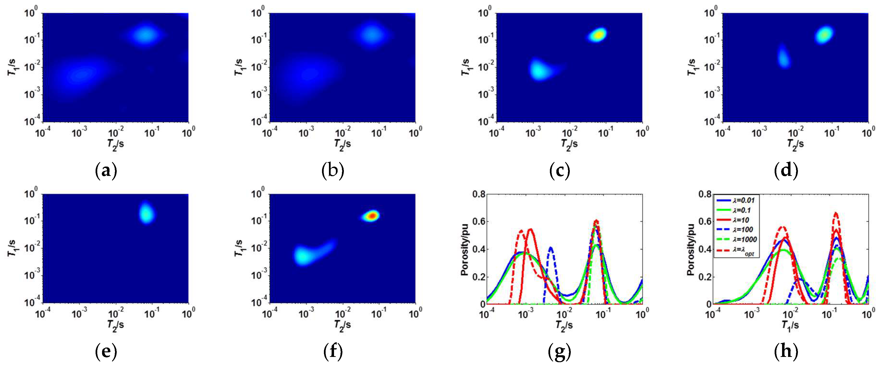
The regularization parameter determines the weight of the residual term and the penalty term in the objective function and plays an important role in T1–T2 spectra inversion. Thus, it is necessary to find the optimal regularization parameter during the T1–T2 spectra inversion. The residuals with different L1 regularization parameters for the compressed echo data were calculated and then the diagram of the logarithmic relationship between the residual and the L1 regularization parameter was plotted, as shown in Figure 10. The corresponding at the red point, where the residual is the minimum, represents the optimal L1 regularization parameter, where . Moreover, five other regularization parameters (0.01, 0.1, 10, 100 and 1000) were tested. The compressed echo data were inverted using the TIST algorithm with the six regularization parameters to obtain the corresponding T1–T2 spectra, as shown in Figure 11a–f. Figure 11g,h show the T2 and T1 spectra from the T1–T2 spectra projections onto the T2 and T1 axes, respectively.
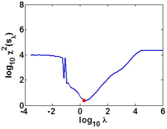
Figure 10.
Diagram of the logarithmic relationship between the residual and the L1 regularization parameter for the compressed echo data.
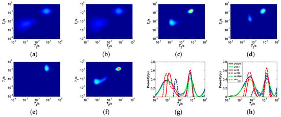
Figure 11.
Inverted T1–T2 spectra, T1 spectra and T2 spectra in heavy oil reservoirs with different regularization parameters. (a–f) represent the inverted T1–T2 spectra with regularization parameters of 0.01, 0.1, 10, 100, 1000 and 1.9156, respectively (g,h) represent the T2 and T1 spectra from the T1–T2 spectra projections onto the T2 and T1 axes, respectively.
Figure 11 indicated that the inverted T1–T2 spectra show some false peaks and the heavy oil signal and water signal exhibit divergences when is far lower than 1.9156. In contrast, the peak of the heavy oil signal gradually narrows and moves along the direction of increase in T1 and T2 and the intensity of the heavy oil signal decreases gradually until the signal disappears in the inverted T1–T2 spectra as the L1 regularization parameter increases when is larger than 1.9156. The inverted T1–T2 spectra with the optimal L1 regularization parameter () is superior to that with the other L1 regularization parameter. L1 regularization term is used to constrain the sparsity of the inverted T1–T2 spectra. When the regularization parameter is smaller, the solution of the objective function is mainly constrained by the residual term and is weakly affected by the penalty term, thus it exhibits the divergence of the fluid signal in the inverted T1–T2 spectra. When the regularization parameter is larger, the solution is mainly affected by the penalty term, which may exhibit excessively sparse fluid signal and also may miss the fluid signal. Comprehensively, an appropriate L1 regularization parameter is a major factor for obtaining accurate inverted T1–T2 spectra using the TIST algorithm.
5. Conclusions and Prospects
In this paper, some commonly used T1–T2 spectra inversion algorithms were compared by way of numerical simulations and the TIST algorithm was selected for NMR data inversion in heavy oil reservoirs. Subsequently, NMR T1–T2 experiments for a disordered accumulation of glass beads saturated with heavy oil and distilled water were implemented. The experimental data were processed and the inverted T1–T2 spectra with different acquisition parameters and inversion parameters employing the TIST algorithm were analyzed, whose aim is to determine the parameter conditions for the optimal T1–T2 spectra of heavy oil reservoirs. The following conclusions were drawn:
The selection of appropriate acquisition parameters is important for obtaining accurate T1–T2 spectra of heavy oil reservoirs. The quality of the T1–T2 spectra in heavy oil reservoirs depends on the number of echo train when the maximum and minimum wait times were fixed and a number no less than 7 is appropriate. If an inappropriate wait time group is used for the T1–T2 measurement, the projected T2 spectra from T1–T2 spectra can still be used for reservoir evaluations. The peak of the heavy oil signal gradually moves along the direction of increase in the T2 and the intensity of the heavy oil signal gradually decreases as the echo spacing increases. To obtain the optimal T1–T2 spectra, the echo spacing should be as small as possible for the T1–T2 measurements in heavy oil reservoirs on the premise that the NMR instrument operate normally.
The TIST algorithm is robust for NMR T1–T2 spectra inversion. However, the inverted T1–T2 spectra in heavy oil reservoirs may be inaccurate if the inversion parameters are inappropriate. A convergence tolerance that is too large or a maximum number of iterations that is too small may both result in exiting the iteration prematurely during the inversion and thus result in inaccurate inversion results. In contrast, a convergence tolerance that is too small or a maximum number of iterations that is too large may both result in redundant iterations and in a time-consuming inversion process. A convergence tolerance of 1 × 10⁻⁷ and a maximum number of iterations of 30,000 are recommended for T1–T2 spectra inversions of heavy oil reservoirs. An appropriate L1 regularization parameter is a major factor for obtaining accurate T1–T2 spectra of heavy oil reservoirs using the TIST algorithm. When a smaller L1 regularization parameter is used, the inverted T1–T2 spectra exhibit divergent signals and some false peaks. When a larger L1 regularization parameter is used, the heavy oil signal narrows, weakens and may be lost in the T1–T2 spectra.
The results and conclusions of this study were obtained using the TIST algorithm based on the NMR T1–T2 experiments of a disordered accumulation of glass beads saturated with heavy oil and distilled water. However, the viscosity of heavy oil is not uniform and dissolved gas can be presented in heavy oil reservoirs. The actual T1–T2 spectra in heavy oil reservoirs are far more complex than the experimental model used in this study. Therefore, future research on T1–T2 spectra in heavy oil reservoirs should focus on more complex models. Moreover, the relaxation time of heavy oil is very short and the development of other pulse sequences that can measure shorter relaxation times is required for in-depth studies of T1–T2 responses of heavy oil reservoirs.
Author Contributions
Conceptualization, R.X. and L.X.; Formal analysis, J.G., R.X. and L.X.; Methodology, J.G. and R.X.; Supervision, R.X. and L.X.; Validation, M.L. and L.G.; Writing—original draft, J.G. and R.X.; Writing—review & editing, J.G., R.X. and L.X.
Funding
This research received no external funding.
Acknowledgments
The work was supported by the National Natural Science Foundation of China under the grant number: 41674126.
Conflicts of Interest
The authors declare no conflict of interest.
Appendix A
This appendix describes TSVD implementation. TSVD algorithm is usually used to find a reasonable solution of the linear least squares problem by removing smaller singular values characterizing the measuring error [17,18,19,20]. The singular values of the kernel matrix K are obtained from SVD
In practice, the smaller singular values affect the stability of the solution and if they are removed, the ill-condition of the matrix would be reduced but the more singular values are removed, the more valuable information will be lost. Hence, choosing the truncated singular value is crucial for the TSVD algorithm. In this paper, we chose the truncated singular value based on data signal-to-noise ratio (SNR) and removed the singular value that is less than . Therefore, the solution of Equation (4) can be written as:
Appendix B
This appendix describes two algorithms for solving L2 regularization problem. Based on Equation (6), the objective function of the L2 regularization method for the NMR data inversion can be written as:
where F is the derivative operator. When F is the identity matrix, L2 regularization is also known as norm smoothing and when F is the second-order derivative operator, L2 regularization is also known as curvature smoothing.
BRD algorithm [37] is usually used to solve the objective function of norm smoothing and the problem can be transformed to search the minimum value of the following convex function
We updated s value by
where ; and are the first and second derivate of the function ; is the first value in the geometric sequence that satisfying
Usually, when the calculated value satisfies Equation (A7), we will terminate the search
where tol is a small fixed value.
LM algorithm [25,30,38] is usually used for solving the objective function of curvature smoothing. And we calculated the new value according to the following equation
where and are the gradient and Hessian matrix of the objective function Equation (A3) and is constantly updated at each iteration, as written
where ; ; and . In this paper, we used S-curve method to choose the regularization parameter of curvature smoothing.
Appendix C
This appendix describes solving algorithm for L1 regularization problem and chosen method for the optimal L1 regularization parameter. Based on Equation (6), the objective function of the L1 regularization method for the NMR data inversion can be written as:
To date, the L1 regularization problem Equation (A10) in NMR data inversion has been solved by a one-step iterative algorithm whose solution is only affected by the solution of the previous step at each iteration, such as the IST algorithm and the primal-dual hybrid gradient algorithm [26,27]. To improve the inversion speed, we used a TIST algorithm [28,39] to solve the objective function Equation (A10). The TIST algorithm employs the following iteration scheme:
where and are the iterative steps, is the tth iterative solution; is the soft thresholding function and .
Monotonicity is an important condition for guaranteeing convergence of the algorithm. Thus, we would implement the following iteration for ,
where is given by Equation (A11); and is the objective function value at iteration number t−1.
The detailed steps of the TIST algorithm are shown below: (1) Input the regularization parameter and the iterative steps and and set the maximum number of iterations itermax and the convergence tolerance tol. (2) Initialize and compute the initial value of the objective function . (3) Compute and the negative elements in are zeroed; subsequently, compute the value of the objective function and let the iteration number t = 2. (4) Compute vector and the nonzero elements in X are set to 1; then re-compute and . (5) Compute and ; the negative elements in are zeroed; if , we re-compute and . Subsequently, the accuracy and let the iteration number t = t + 1. (6) If or , stop the iteration and output , else go to step (4) and start a new iteration.
To choose the optimal L1 regularization parameter, we computed the residual for different regularization parameters, where is the solution of the objective function with the regularization parameter . The corresponding with the minimum residual is considered as the optimal solution of Equation (A10), thus the corresponding is the optimal L1 regularization parameter.
References
- Galford, J.E.; Marschall, D.M. Combining NMR and Conventional Logs to Determine Fluid Volumes and Oil Viscosity in Heavy-oil Reservoirs. In Proceedings of the SPE Annual Technical Conference and Exhibition, Dallas, TX, USA, 1–4 October 2000. [Google Scholar]
- Smith, C.K.; Wang, F.H.L. Sampling and Characterization of Rocks and Fluids for Heavy-oil Reservoir Management. In Proceedings of the SPE Annual Technical Conference and Exhibition, Denver, CO, USA, 21–24 September 2008. [Google Scholar]
- Liu, H.; Xiao, L.; Guo, B.; Zhang, Z.; Zong, F.; Deng, F.; Yu, H.; Anferov, V.; Anferova, V. Heavy Oil Component Characterization with Multi-dimensional Unilateral NMR. Petrol. Sci. 2013, 10, 402–407. [Google Scholar] [CrossRef]
- Xin, X.; Yu, G.; Chen, Z.; Wu, K.; Dong, X.; Zhu, Z. Effect of Non-Newtonian Flow on Polymer Flooding in Heavy Oil Reservoirs. Energies 2018, 10, 1225. [Google Scholar] [CrossRef] [PubMed]
- Coates, G.R.; Xiao, L.; Prammer, M.G. NMR Logging: Principles and Applications; Gulf Professional Publishing: Houston, TX, USA, 1999. [Google Scholar]
- LaTorraca, G.A.; Dunn, K.J.; Webber, P.R.; Carison, R.M.; Stonard, S.W. Heavy Oil Viscosity Determination Using NMR Logs. In Proceedings of the SPWLA 40th Annual Logging Symposium, Oslo, Norway, 30 May–3 June 1999. [Google Scholar]
- Bryan, J.; Kantzas, A.; Bellehumeur, C. Oil-viscosity Predictions from Low-field NMR Measurements. SPE Reserv. Eval. Eng. 2005, 8, 44–52. [Google Scholar] [CrossRef]
- Guo, J.; Xie, R. Numerical Simulation and Parameter Analysis of NMR T2–D Distributions of Tight Sandstone Saturated with a Gas–water Two-phase Fluid. J. Nat. Gas Sci. Eng. 2017, 37, 502–511. [Google Scholar] [CrossRef]
- Zhu, L.; Zhang, C.; Wei, Y.; Zhou, X.; Huang, Y.; Zhang, C. Inversion of the Permeability of a Tight Gas Reservoir with the Combination of a Deep Boltzmann Kernel Extreme Learning Machine and Nuclear Magnetic Resonance Logging Transverse Relaxation Time Spectrum Data. Interpretation 2017, 5, T341–T350. [Google Scholar] [CrossRef]
- Kleinberg, R.L.; Vinegar, H.J. NMR Properties of Reservoir Fluids. Log Anal. 1996, 37, 20–32. [Google Scholar]
- Freedman, R.; Johnston, M.; Morriss, C.E.; Straley, C.; Tutunjian, P.N.; Vinegar, H.J. Hydrocarbon Saturation and Viscosity Estimation from NMR Logging in the Belridge Diatomite. Log Anal. 1997, 38, 44–59. [Google Scholar]
- Mirotchnik, K.; Allsopp, K.; Kantzas, A. Low-field NMR Method for Bitumen Sands Characterization: A New Approach. SPE Reserv. Eval. Eng. 1999, 4, 88–96. [Google Scholar] [CrossRef]
- Wayne, C.; Doug, W. A Special Application of NMR Logging to Detect Heavy Oil on North Slope Satellite Fields, Alaska. In Proceedings of the SPE Western Regional Meeting, Anchorage, AK, USA, 26–27 May 1999. [Google Scholar]
- Sun, B.Q.; Olson, M.; Baranowski, J.; Chen, S.; Li, W. Direct Fluid Typing and Quantification of Onorico Belt Heavy Oil Reservoirs Using 2D NMR Logs. In Proceedings of the SPWLA 47th Annual Logging Symposium, Veracruz, Mexico, 4–7 June 2006. [Google Scholar]
- Chen, S.; Mette, M.; Jumagaziyev, D.; Shao, W.; Nina, A.B. Application of NMR Logging for Characterizing Movable and Immovable Fractions of Viscose Oils in Kazakhstan Heavy Oil Fields. In Proceedings of the SPWLA 47th Annual Logging Symposium, Veracruz, Mexico, 4–7 June 2006. [Google Scholar]
- Enninful, H.R.N.B.; Babak, P.; Kantzas, A.; Bryan, J. Fluid Quantification in Oil Sands Using a 2D NMR Spectroscopy. In Proceedings of the 13th Offshore Mediterranean Conference Exhibition, Ravenna, Italy, 29–31 March 2017. [Google Scholar]
- Prammer, M.G. NMR Pore Size Distributions and Permeability at the Well Site. In Proceedings of the SPE Annual Technical Confernce Exhibition, New Orleans, LO, USA, 25–28 September 1994. [Google Scholar]
- Zhou, X.; Nie, S.; Wang, Y.; Zhang, Y.; Yang, Y.; Yang, P. An Iterative Truncated Singular Value Decomposition (TSVD)-based Inversion Methods for 2D NMR. Chin. J. Magn. Reson. 2013, 30, 541–551. [Google Scholar]
- Ge, X.; Fan, Y.; Chen, H.; Deng, S.; Cao, Y.; Zahid, M.A. Probing the Influential Factors of NMR T1-T2 Spectra in the Characterization of the Kerogen by Numerical Simulation. J. Magn. Reson. 2015, 260, 54–66. [Google Scholar] [CrossRef]
- Ge, X.; Wang, H.; Fan, Y.; Cao, Y.; Chen, H.; Huang, R. Joint Inversion of T1-T2 Spectrum Combining the Iterative Truncated Singular Value Decomposition and the Parallel Particle Swarm Optimization Algorithms. Comput. Phys. Commun. 2016, 198, 59–70. [Google Scholar] [CrossRef]
- Song, Y.; Venkataramanan, L.; Hurlimann, M.; Flaum, M.; Frulla, P.; Straley, C. T1–T2 Correlation Spectra Obtained Using a fast two-dimensional Laplace Inversion. J. Magn. Reson. 2002, 154, 261–268. [Google Scholar] [CrossRef]
- Venkataramanan, L.; Song, Y.; Hurlimann, M.D. Solving Fredholm Integrals of the First Kind with Tensor Product Structure in 2 and 2.5 Dimensions. IEEE Trans. Signal Process. 2002, 50, 1017–1026. [Google Scholar] [CrossRef]
- Sun, B.; Dunn, K.J. A Global Inversion Method for Multi-dimensional NMR Logging. J. Magn. Reson. 2005, 172, 152–160. [Google Scholar] [CrossRef]
- Chouzenoux, É.; Moussaoui, S.; Idier, J.; Mariette, F. Efficient Maximum Entropy Reconstruction of Nuclear Magnetic Resonance T1-T2 Spectra. IEEE Trans. Signal Process. 2010, 58, 6040–6051. [Google Scholar] [CrossRef]
- Zou, Y.; Xie, R.; Ding, Y.; Arad, A. Inversion of Nuclear Magnetic Resonance Echo Data Based on Maximum Entropy. Geophysics 2016, 81, D1–D8. [Google Scholar] [CrossRef]
- Zhou, X.; Su, G.; Wang, L.; Nie, S.; Ge, X. The Inversion of 2D NMR Relaxometry Data Using L1 Regularization. J. Magn. Reson. 2017, 275, 46–54. [Google Scholar] [CrossRef]
- Reci, A.; Sederman, A.J.; Gladden, L.F. Obtaining Sparse Distributions in 2D Inverse Problems. J. Magn. Reson. 2017, 281, 188–198. [Google Scholar] [CrossRef]
- Guo, J.; Xie, R.; Liu, M. A Robust Algorithm for 2-D NMR Diffusion-relaxation Spectra Inversion. IEEE Geosci. Remote Sens. Lett. 2018, 15, 1545–1549. [Google Scholar] [CrossRef]
- Berman, P.; Levi, O.; Parmet, Y.; Saunders, M.; Wiesman, Z. Laplace Inversion of Low-resolution NMR Relaxometry Data Using Sparse Representation Methods. Concept. Magn. Reson. Part A 2013, 42, 72–88. [Google Scholar] [CrossRef]
- Guo, J.; Xie, R.; Zou, Y.; Jin, G.; Gao, L.; Xu, C. A New Method for NMR Data Inversion Based on Double-parameter Regularization. Geophysics 2018, 83, JM39–JM49. [Google Scholar] [CrossRef]
- Guillen, A.; Legchenko, A. Inversion of Surface Nuclear Magnetic Resonance Data by An Adapted Monte Carlo Method Applied to Water Resource Characterization. J. Appl. Geophys. 2002, 50, 193–205. [Google Scholar] [CrossRef]
- Prange, M.; Song, Y. Quantifying Uncertainty in NMR T2 Spectra Using Monte Carlo Inversion. J. Magn. Reson. 2009, 196, 54–60. [Google Scholar] [CrossRef]
- Salazar, R.; Sun, B. Monte Carlo Optimization-inversion Methods for NMR. Petrophysics 2010, 51, 208–218. [Google Scholar]
- Hürlimann, M.D.; Venkataramanan, L. Quantitative Measurement of Two-dimensional Distribution Functions of Diffusion and Relaxation in Grossly Inhomogeneous Fields. J. Magn. Reson. 2002, 157, 31–42. [Google Scholar] [CrossRef]
- Ailon, N.; Liberty, E. Fast Dimension Reduction Using Rademacher Series on Dual BCH Codes. Discret. Comput. Geom. 2009, 42, 615. [Google Scholar] [CrossRef]
- Guo, J.; Xie, R.; Jin, G. An Efficient Method for NMR Data Compression Based on Fast Singular Value Decomposition. IEEE Geosci. Remote Sens. Lett. 2019, 16, 301–305. [Google Scholar] [CrossRef]
- Butler, J.; Reeds, J.; Dawson, S. Estimating Solutions of First Kind Integral Equations with Nonnegative Constraints and Optimal Smoothing. SIAM J. Numer. Anal. 1981, 18, 381–397. [Google Scholar] [CrossRef]
- Press, W.H.; Teukolsky, S.A.W.; Vetterling, T.; Flannery, B.P. Numerical Recipes: The Art of Scientific Computing, 3rd ed.; Cambridge University Press: Cambridge, UK, 2007. [Google Scholar]
- Bioucas-Dias, J.M.; Figueiredo, M.A.T. A New TwIST: Two-step Iterative Shrinkage/Thresholding Algorithms for Image Restoration. IEEE Trans. Image Process. 2007, 16, 2992–3004. [Google Scholar] [CrossRef]
© 2019 by the authors. Licensee MDPI, Basel, Switzerland. This article is an open access article distributed under the terms and conditions of the Creative Commons Attribution (CC BY) license (http://creativecommons.org/licenses/by/4.0/).


