Article

Integrated Wind Farm Power Curve and Power Curve Distribution Function Considering the Wake Effect and Terrain Gradient

1
School of Electrical Engineering, Southeast University, Nanjing 210096, China
2
Departamento de Enxeñería Eléctrica, Universidade de Vigo, Campus de Lagoas, 36310 Vigo, Spain
3
Department of Electronic Engineering, Royal Holloway, University of London, Egham TW20 0EX, UK
4
Department of Electronics and Communication Engineering, Visvesvaraya National Institute of Technology, Nagpur 440010, India
*
Author to whom correspondence should be addressed.
Energies 2019, 12(13), 2482; https://doi.org/10.3390/en12132482
Submission received: 6 June 2019 / Revised: 22 June 2019 / Accepted: 26 June 2019 / Published: 27 June 2019
(This article belongs to the Special Issue Wind Farm Power Curves and Power Distributions)

Abstract

:
This work presents a computational method for the simulation of wind speeds and for the calculation of the statistical distributions of wind farm (WF) power curves, where the wake effects and terrain features are taken into consideration. A three-parameter (3-P) logistic function is used to represent the wind turbine (WT) power curve. Wake effects are simulated by means of the Jensen’s wake model. Wind shear effect is used to simulate the influence of the terrain on the WTs located at different altitudes. An analytical method is employed for deriving the probability density function (PDF) of the WF power output, based on the Weibull distribution for describing the cumulative wind speed behavior. The WF power curves for four types of terrain slopes are analyzed. Finally, simulations applying the Monte Carlo method on different sample sizes are provided to validate the proposed model. The simulation results indicate that this approximated formulation is a possible substitute for WF output power estimation, especially for the scenario where WTs are built on a terrain with gradient.

1. Introduction

To date, wind energy has become a promising alternative and renewable energy resource to handle the problem of energy crisis and environmental deterioration. Along with the rapid development and extensive exploitation of wind energy throughout the world, calculations of the output power of wind farm (WF)s is widely required not only for the WF layout optimization problem [1,2] but for the WF output monitoring [3,4,5], analysis [6], prediction [7,8], and control [9,10,11,12,13] problems. However, in most of the literature, the wind turbine (WT) power curves are mathematically expressed by means of a piecewise function. For a certain inflow wind speed, wind speeds experienced by different WTs on a WF differ for several reasons. One of the major influencing factors is the wake effect and another may be the altitude differences of the WTs’ positions. Therefore, representation of the WF power curves should not be simply acquired as the summation of power curves produced by the individual WTs.
First of all, the power curves of a WT not only indicate the performance of the WT, but also serve as a reference for prediction, if accurately modeled [14,15]. Therefore, in order to obtain WF power curves, accurate models for WT power curves must be dealt with first. The WT power curve models are commonly classified as parametric or nonparametric. In [4] it is proven that the parametric least squares model and the nonparametric k-nearest neighbor model present high accuracy. In [5] a parametric power curve was developed, that could be applied for control, monitoring, prediction, and optimization of WF performance. A comparison of several WT power curve modeling methods and a critical analysis of then is available in [16]. In [17] the estimation of the WT power curve was operated on the basis of cluster center fuzzy logic modelling. In 2016, Pelletier [18] used an artificial neural network to model WT power curves. In 2017, Ouyang [19] proposed a data partitioning and mining approach for WT power curve modeling. In 2018, Zhao et al. [20] developed a data-driven correction method for the refinement of a WF power curve under wind curtailment and the work in [20] presented the ability to be directly used in different cases without the need to tune any parameters, for WTs and also for WFs.
On the basis of the extensive research on WT power curves, many previous works have established WF power curve distributions taking wake effect into consideration. In 2014, Shi et al. [21] developed a solution based on a probability analysis for modeling WF power output. In the cited paper, wake effect was taken into consideration by using the Jensen’s model and the WF power probability density function (PDF) was deduced with the help of an analytical method. Feijóo et al. were inspired by [21] and combined this with [22] to deduce WF power curve models and power probability density models with three and four parameters in 2017, [23] and [24] respectively. One of the advantages of using these models is that they are not piecewise, which differs from other proposals, such as [21]. Moreover, the wake deficit of the whole WF is synthesized to be represented by one wake coefficient which avoids the computational complexity of calculating the wake deficit one by one. In addition, in [25], four major wind directions were taken into account for the approximation of the WF output power calculation which further refined this model.
As is pointed out in [23,24,25], it is advantageous to utilize these models in view of their simplicity as compared with other proposals and to preserve accuracy. In addition, wake effects are already synthesized in the expression of total power and WF power PDF. Nonetheless, the major deficiency of these models is that they can only be applied in the case where the WTs are installed on flat land. If the WF is located on a hilly area where the positions of the WTs form a gradient, then these models cannot be directly applied to calculate the total output power of the WF which results in an increase of the computation error. Thus, in this case, if these simplified models are to be used a modification needs to be added beforehand.
This work is based on the advantages of the aforementioned models and is organized as follows: First, Jensen’s wake model is introduced and then the analytical wake model is given which takes the height differences between WTs into consideration. Secondly, an integrated three parameter (3-P) power distribution function of a WF is established which is classified into four sub-models according to the value of the hill’s slope. Finally, this model is proven by simulations and comparison with the Monte Carlo simulation results.

2. Wake Analysis

2.1. Wake Model

On a WF with multiple rows of WTs, the presence of a WT affects the wind speed downstream. This aerodynamic fact is called wake effect. The wake effect of a WT is depicted by using the Jensen’s model [26,27] as shown in Figure 1.
{ ρ π R r 2 v 1 + ρ ( π R w 2 π R r 2 ) v 0 = ρ π R w 2 v x d R w d t = K d R w d x = d R w d t d t d x = K v x
where, Rr is the length of a WT blade and Rw is the radius of the wake area caused by WT1 at distance x, ρ is the air density, v0 is the ambient wind speed, and K is the wake decay constant as is shown in Figure 1.
The wind speed, vx, on WT2 is calculated according to Equation (2).
v x = v 0 ( 1 ξ )
ξ = ( 1 1 C t ) ( R r R r + K x ) 2
where, ξ is the wake coefficient and Ct are the thrust coefficients of the WT.

2.2. Shear Effect

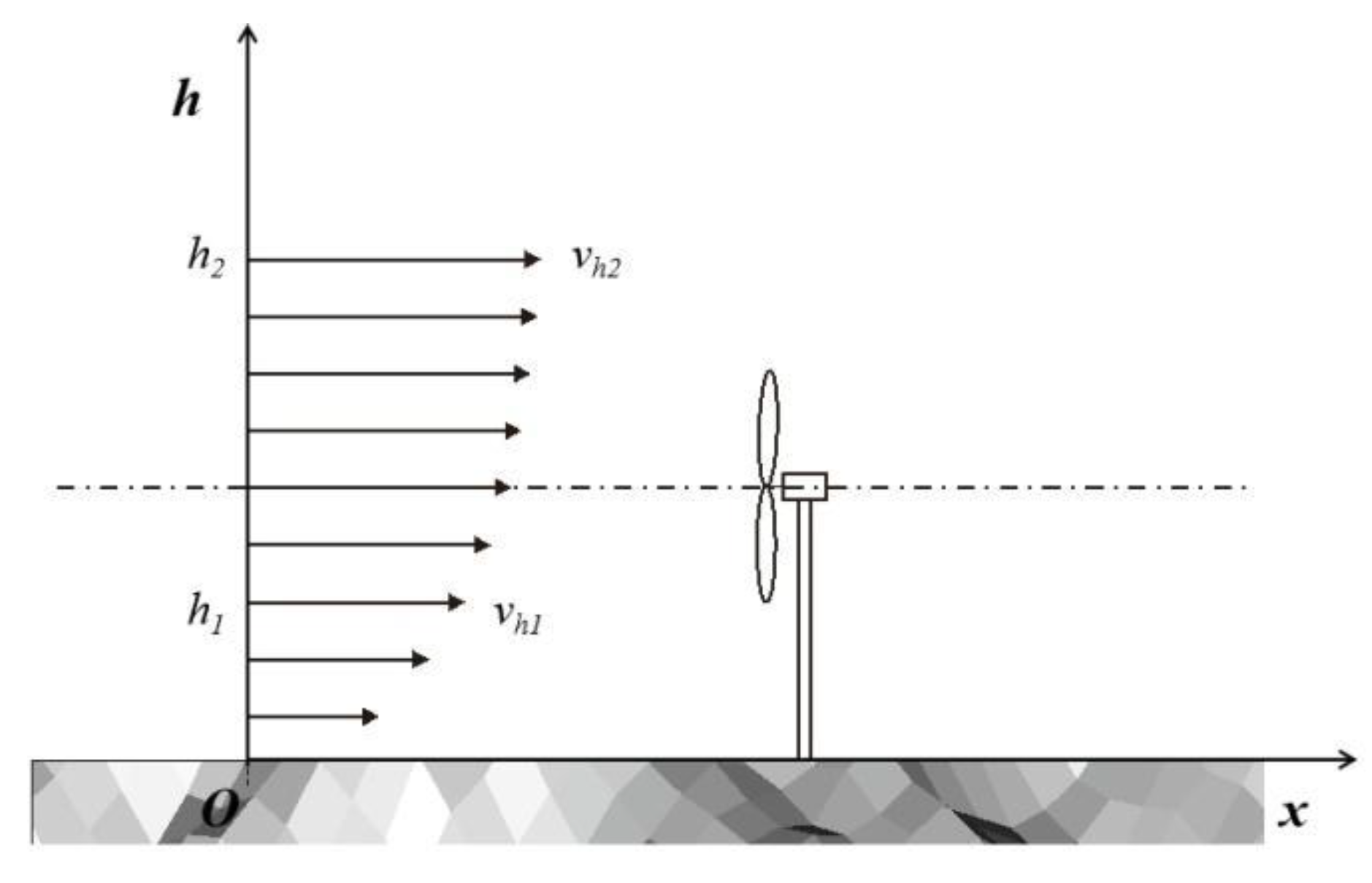
In real situations, wind speed depends on height, which is known as wind shear, according to the influence of the boundary layer fluid flow. As depicted and shown in Figure 2, the wind vertical distribution curve exhibits a certain pattern, such as a logarithmic curve or a cubic curve. Many factors influence the shape of this curve, majorly the roughness of ground. The rougher the ground is, the slower the wind close to the ground is.
The distribution of the obtained wind shear values is effectively approximated by the following expression [28]:
v ( z ) = v ( z r e f ) ( z z r e f ) α h
where, v(z) is the wind speed at height z, v(zref) is the wind speed at the height zref where it is measured, and α h is the approximation coefficient and is obtained according to Equation (5)
α h = 0.24 + 0.096 log ( z 0 ) + 0.016 [ log ( z 0 ) ] 2
for 0.001 m < z0 < 10 m.

2.3. Wake Analysis and Terrain Gradient

First, let us suppose that the WF with a by b WTs is located at a terrain with a gradient of s. The distance between two adjacent rows is drow. There are four scenarios in total with different gradient values:
Scenario 1 WF on a flat area.
The WF is considered to be located on a flat area (Figure 3), if the slope of the terrain, s, is equal to zero. This scenario was already analyzed in [21] and the conclusion of [21] is directly applied.
In this case, the WTs share the same height. Thus, vx is directly calculated using Equation (2) and the wake coefficient of the ith WT is:
ξ i = [ 1 ( 1 1 C t ) ( R r R r + K d r o w ) 2 ] i 1 ( i = 1 , 2 , , a )
The wind speed at the ith WT is:
v i = v 0 ξ i i = 1 , 2 , , a
The mean value ξ w 0 for all the a rows of the WTs’ wake coefficients 1 , ξ , ξ 2 , , ξ a 1 is calculated as:
ξ w 0 = 1 ξ a a ( 1 ξ )
Scenario 2 WF over a hill with gentle gradient.
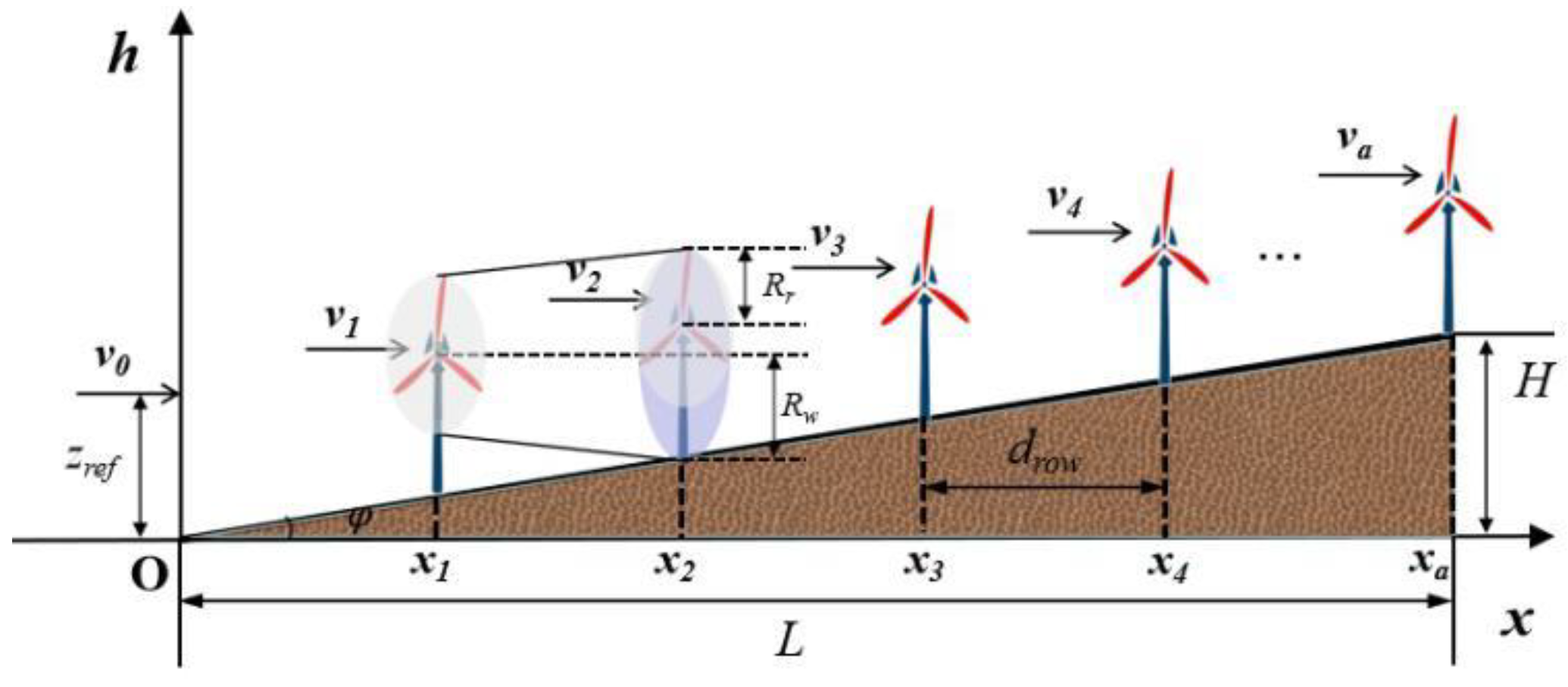
When the slope of the terrain is gentle, the WTs located at downstream positions are totally affected by the wake of upstream WTs (Figure 4).
In other words, the slope must meet the following condition:
d h R w R r
Namely,
s = H L K
That is to say, if the slope of the hill, s, is lower or equal to the wake decay constant, K, then the wind speed of the downstream WT is calculated as in Equation (11).
v x = v 0 [ 1 ( 1 1 C t ) ( R r ( R r + K x ) ) 2 ] ( z z r e f ) α h
where, x = d r o w and z = d r o w s i ( i = 1 , 2 , , a ) .
The wake coefficient of the ith WT is:
ξ d i = [ 1 ( 1 1 C t ) ( R r R r + K d r o w ) 2 ] ( d r o w s i z r e f ) α h ( i = 1 , 2 , , a )
Thus, the wind speed of the ith WT is:
v i = v 0 j = 1 i ξ d j     i = 1 , , a
For simplicity, let
ξ d i = C 1 i α h ( i = 1 , 2 , , a )
where, C 1 = [ 1 ( 1 1 C t ) ( R r R r + K d r o w ) 2 ] ( d r o w s z r e f ) α h .
Scenario 3 WF over a hill with moderate gradient.
When the slope of the terrain is moderate, the WTs located at downstream positions are partially affected by the wake of upstream WTs (Figure 5).
This means the slope must meet the following condition:
R w R r < d h R w + R r
Namely,
K < s 2 R r d r o w + K
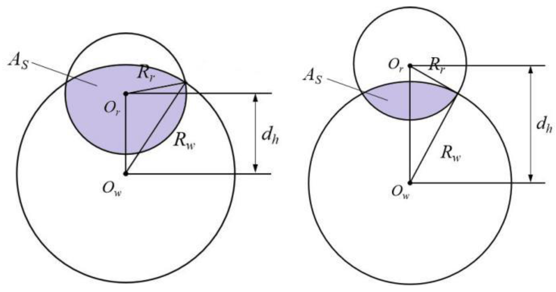
In this scenario, the downstream WT2 vertically deviates the upstream WT1 due to the shape of the terrain. WT2 may be incompletely covered by WT1′s wake. The area of the shadow on WT2 covered by WT1′s wake is shown in Figure 5 when considering terrain gradient.
The area of the shadow in Figure 6 is calculated as in [29]:
A S = arccos ( R w 2 + d h 2 R r 2 2 R w d h ) R w 2 + arccos ( R r 2 + d h 2 R w 2 2 R r d h ) R r 2 sin [ arccos ( R w 2 + d h 2 R r 2 2 R w d h ) ] R w d h
The height difference of two WTs is calculated as follows:
d h = d r o w s
The wind speed of the downstream WT is calculated as follows:
v x = v 0 [ 1 ( 1 1 C t ) ( R r ( R r + K x ) ) 2 ( A S π R r 2 ) ] ( z z r e f ) α h
where, x = d r o w and z = d r o w s i ( i = 1 , 2 , , a ) .
Thus, the wind speed of the ith WT is:
v i = v 0 j = 1 i ξ d j i = 1 , , a
The wake coefficient of the ith WT is:
ξ d i = [ 1 ( 1 1 C t ) ( R r R r + K d r o w ) 2 ( A S π R r 2 ) ] ( z z r e f ) α h ( i = 1 , 2 , , a )
For simplicity, let
ξ d i = C 2 i α h ( i = 1 , 2 , , a )
where, C 2 = [ 1 ( 1 1 C t ) ( R r R r + K d r o w ) 2 ( A S π R r 2 ) ] ( d r o w s z r e f ) α h .
Scenario 4 WF over a hill with steep gradient.
When the slope of the terrain is steep, wakes do not affect the WTs located at downstream positions (Figure 7).
This means the slope must meet the following condition:
d h > R w + R r
Namely,
s > 2 R r d r o w + K
In this case, there is no wake influence between any two WTs. Thus, the only factor influencing the wind speed is shear effect.
The wind speed of the ith WT is calculated as follows:
v i = v 0 ( z z r e f ) α h = v 0 ( d r o w s i z r e f ) α h     i = 1 , 2 , , a
It should be noted that this scenario excludes the case where the gradient is extremely steep and the mountain itself blocks airflow while wake effect between WTs at different heights does not occur.
According to the Betz limit [30], if the WT extracts 100% of the wind energy, the air behind the WT does not move, which creates a “wall” and stops further wind from passing through the WT. At a fixed free wind speed, the distance of the WT’s blade to the “wall” determines the inflow wind speed on the WT blades which is reduced by a restrained path of outflow.

3. WF PDF

3.1. 3-P WT PDF Model

Three models for WT power curves and WT PDFs were proposed in [22], on the basis of the logistic function, which is continuous. The one called 3-P-DP is mathematically expressed by means of Equation (26).
P ( v ) = P r ( 1 + exp ( 4 s v ( v i p v ) P r ) ) 1
where, Pr is the rated power of the WT, s v = d P d v | v = v i p , vip the value of the wind speed at the inflection point of the power curve, and v is the inflow wind speed of the WT.
If the inflow wind speed is regarded as a random variable which follows a Weibull distribution with a scale parameter C and a shape parameter k, i.e., f v ( v ) = k C ( v C ) k 1 e ( v C ) k , then the PDF of the WF output power is obtained using the change of variable technique [31]:
f P ( P ) = k C ( v i p P r 4 s v ln ( P r P 1 ) C ) k 1 | P r 2 4 s v P ( P r P ) |
The advantage of utilizing Equations (26) and (27) is that they are continuous functions, unlike the piecewise function which has been proposed in other papers.

3.2. 3-P WF PDF Model

Consider a WF with a row, b column layout for a WF, and let drow be the space existing between two different WTs. In this case, an equivalent model for the WF power is proposed by assuming all the WTs of one column are located in a row. The proposal supposes a unidirectional wind speed.
Scenario 1 WF on a flat area (s = 0).
When the WF is built on a flat area, the total output power of the whole WF is calculated as follows:
P W F 0 ( v 0 ) = a b P r ( 1 + exp ( 4 s v ( v i p ξ w 0 v 0 ) P r ) ) 1
where, ξ w 0 is calculated using Equation (8).
Scenario 2 WF over a hill with gentle gradient ( 0 < s K ).
The total output power of the WF is calculated as:
P W F 1 ( v 0 ) = a b P r ( 1 + exp ( 4 s v ( v i p ξ w 1 v 0 ) P r ) ) 1
where, ξ w 1 is the equivalent wake effect coefficient of the WF with gentle gradient, which is calculated as follows:
ξ w 1 = 1 a ( j = 1 a 1 i = 1 j ξ d i ) = 1 a ( 1 + j = 1 a 1 i = 1 j C 1 i α h ) = 1 a ( 1 + C 1 1 α h + C 1 2 ( 1 2 ) α h + + C 1 a 1 ( 1 2 ( a 1 ) ) α h ) = 1 a ( i = 0 a 1 C 1 i ( i ! ) α h )
where, C1 is the same parameter in Equation (14).
Scenario 3 WF over a hill with medium gradient ( K < s 2 R r d r o w + K ).
Similar to Scenario 2, the total output power of the WF is calculated as:
P W F 2 ( v 0 ) = a b P r ( 1 + exp ( 4 s v ( v i p ξ w 2 v 0 ) P r ) ) 1
where, ξ w 2 is the equivalent wake effect coefficient of the WF over a hill with medium gradient, which is calculated as follows:
ξ w 2 = 1 a ( j = 1 a 1 i = 1 j ξ d i ) = 1 a ( 1 + j = 1 a 1 i = 1 j C 2 i α h ) = 1 a ( 1 + C 2 1 α h + C 2 2 ( 1 2 ) α h + + C 2 a 1 ( 1 2 ( a 1 ) ) α h ) = 1 a ( i = 0 a 1 C 2 i ( i ! ) α h )
where, C2 is the same parameter in Equation (22).
Scenario 4 WF over a hill with steep gradient ( s > 2 R r d r o w + K ).
The power function is different from the above scenarios since there is no wake effect in this scenario. The total output power of the WF is calculated as:
P W F 3 ( v 0 ) = b P r i = 1 a ( 1 + exp ( 4 s v ( v i p v 0 ( d r o w s i z r e f ) α h ) P r ) ) 1

3.3. WF Power PDF

The PDF of the WF output power, now considering wake effect and terrain gradient, for Scenario 1 to Scenario 3 is expressed in Equation (34), by applying the change of variable technique [31]. The PDF of the total WF output power for Scenario 4 is difficult to deduce. Thus, it is not displayed here.
f P W F i ( P W F i ) = k C ( v i p P r 4 s v ln ( a b P r P W F i 1 ) C ξ w i ) k 1 exp ( ( v i p P r 4 s v ln ( a b P r P W F i 1 ) C ξ w i ) k ) | a b P r 2 4 s v ξ w i P W F i ( a b P r P W F i ) | i = 0 , 1 , 2

3.4. Implementation of the WF Output Power Calculation Function

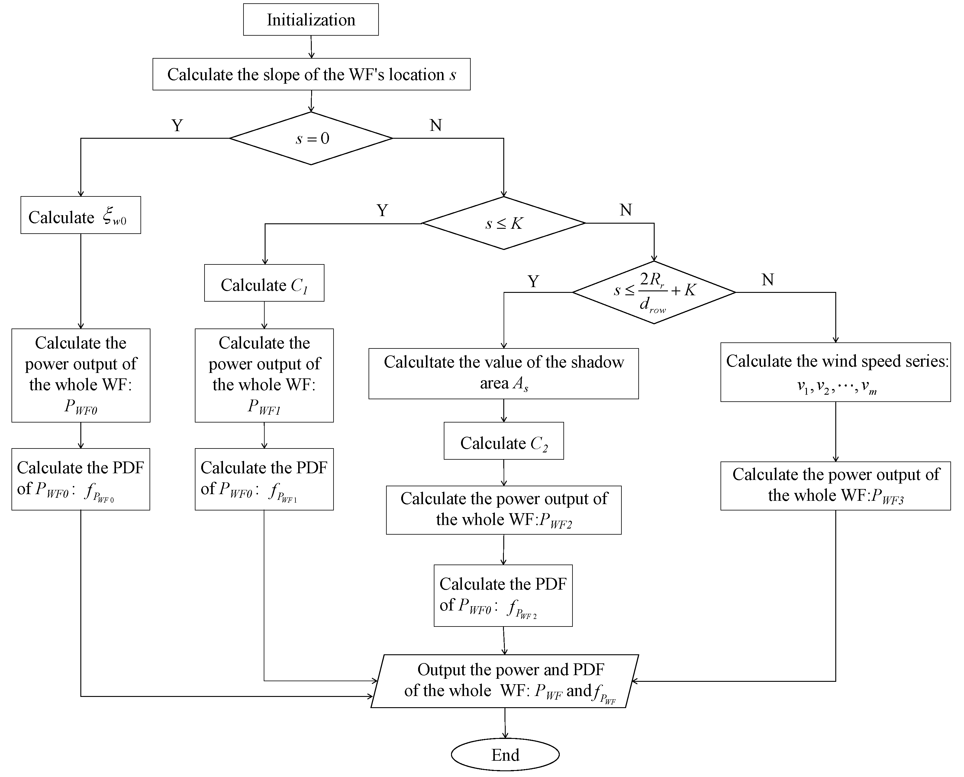
The implementation of this integrated power distribution function is illustrated by the flow chart in Figure 8. There are five main steps in total:
Step 1 
Initialization of the program and input of all the parameters.
Step 2 
Calculation of the terrain’s slope to determine the scenario.
Step 3 
Calculation of the whole WF’s output power using the model for the scenario.
Step 4 
Calculation of the WF output power’s PDF.
Step 5 
Output of the calculated power and PDF of the whole WF.

4. Case Study

Simulations of a 50 MW WF with 25 two MW WTs, in a five by five layout, are presented in this section. The constants are given in Table 1:
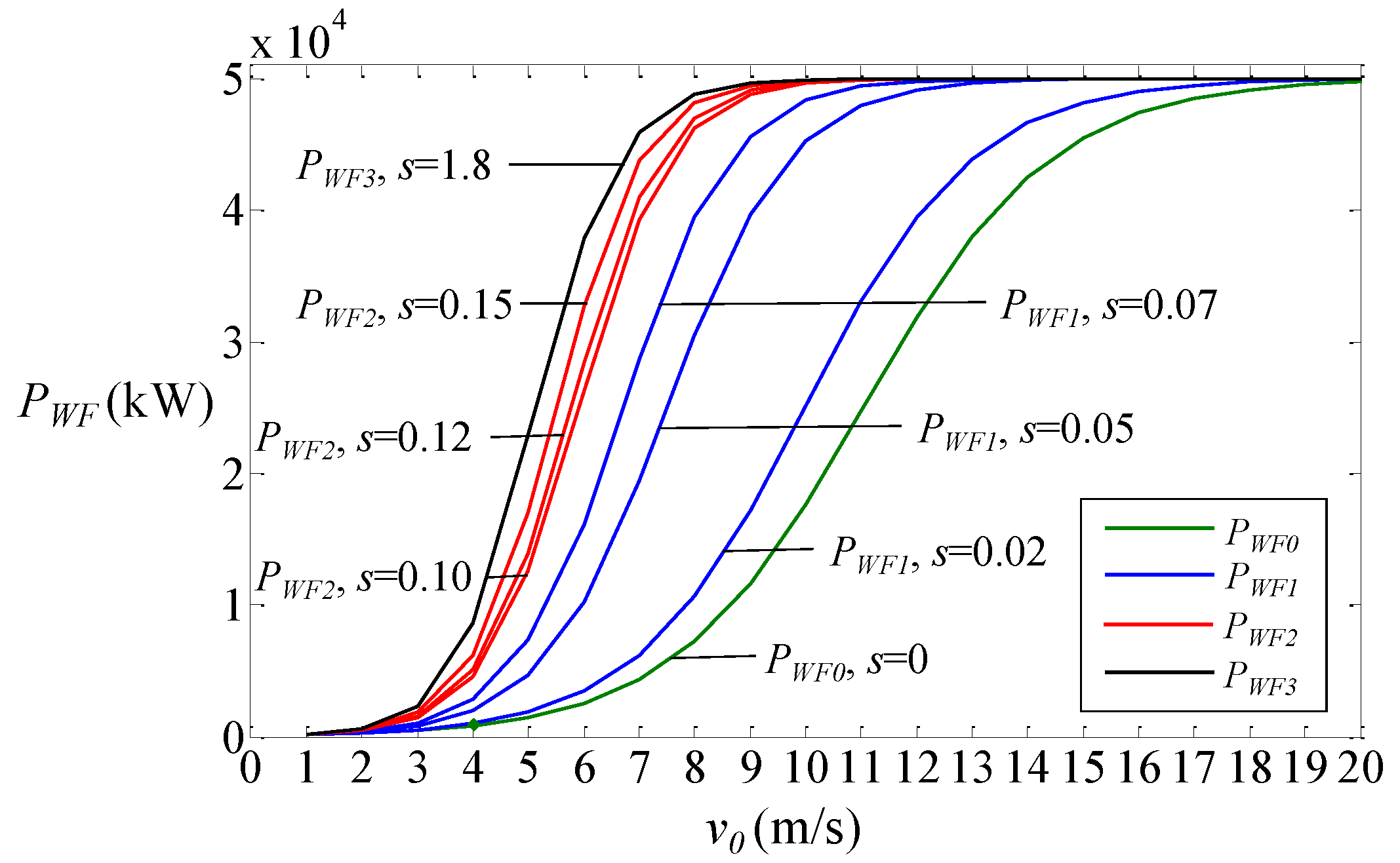
The slope of the hill, s, changes from s = 0 for Scenario 1; s = 0.02, s = 0.05, and s = 0.07 for Scenario 2; s = 0.10, s = 0.12, and s = 0.15 for Scenario 3; and s = 1.8 for Scenario 4.

4.1. Simulation of the WF Power Curve Functions

The simulation results are given below:
It is clearly seen from Figure 9 that, generally, when the gradient of the WF’s location changes, at the same inflow wind speed, the WF with the same layout and same WT type will produce different output power, that is to say, when s grows, PWF also increases in accordance. This phenomenon is explained from two aspects. First, with an increase of the gradient, the coverage areas of wake gradually decrease which gives rise to the reduction of wake loss. Secondly, with the rise of s, an increase of the WTs’ elevation brings about higher wind speed. These two factors synthetically lead to an increase of the WF power output. Another phenomenon is that when s changes from 0 to 0.07, the curves of PWF0 and PWF1 vary dramatically. Nevertheless, when s changes from 0.10 to 1.8, the curves of PWF2 and PWF3 vary to a much lower degree. This implies that the power curve of the WF has a higher sensitivity to the terrain’s gradient if s is small. When the wake is partially covered or not covered, the power curve of the WF is altered much less through a change in s.

4.2. Validation by Means of Monte Carlo Simulations

The Monte Carlo simulation method [32] is utilized for comparisons of precision and computation time. The parameters of the Weilbull distribution function are set to be C = 8m/s and k = 2. The cumulative distribution function (CDF) is chosen instead of the PDF in Equation (34), because it facilitates the comparison.
The basic steps of the Monte Carlo simulation [32] are as follows:
Step 1 Formulation of the probabilistic model according to the problem. The constructed model should be consistent with the actual problem or system in terms of the main characteristic parameters. This must generate a probability distribution function, and this distribution is described by its PDF or CDF. The formulation requires knowing the CDF.
Then, repeat the following process, as many times as needed to have a representative result.
Step 2 Generation of a random number in the interval (0,1) according to a uniform distribution.
Step 3 Use of the inverse of CDF to obtain the value in the desired distribution.
Figure 10 illustrates the results of the cumulative distribution of output power of the whole WF on different slopes (0 for a and b, 0.05 for c and d, and 0.12 for e and f) using the proposed analytical method under different sample sizes (100 for a, c and e; and 50,000 for b, d, and f). The curves in Figure 10 correspond to “calculated power including wake effects”.
From Figure 10, it is revealed that with the growth of sample size, particularly when the sample size is set to be 50,000, the results from the analytical model and the Monte Carlo simulation are almost identical.

5. Conclusions

This paper presents a non-piecewise expression for representing WF power curves considering different terrain gradients. It is based on the previous work by Shi et al. [21] which is based on the Jensen’s wake model [26,27]. The WT power curve is represented by the continuous logistic function [22,23,24,25]. The Monte Carlo simulations are presented to justify the accuracy of the proposed model.
The main improvement and novelty of this study with respect to other works of the same authors is that it includes a much better approach to complex terrain analysis. In previous works [23,24,25] plain terrains were assumed, which can be used in a wide set of cases, but not always. Therefore, this study is considered to be a much more complete work.
The main advantage of using this model is that the wake effect and terrain gradient are already included in the expression of the total power. The only necessary thing is to determine the value of the terrain’s slope and then an integrated power distribution function is selected. Another advantage of using this approach is that this model is simpler than other proposals, and without any loss of accuracy. This helps users reduce the computational complexity of the WF output power calculation, especially when the WF size is large. The proposed analytical WF output power model is easily integrated into WF monitoring, control, and optimization problems.
Future work should focus on the following aspects:
(i)
The scenario where the gradient is extremely steep needs to be studied. The condition of inflow air and outflow air requires detailed analyses, especially when the WTs’ blades are quite close to the mountain “wall”. The corresponding PDF in scenario 4 should be derived.
(ii)
This approximate computation model can only be applied to WFs with a certain orderly arrangement (identical drow for all rows). Improvements and also a challenge for future work is to consider not only more irregular WF layouts but more complex terrains as well.
(iii)
Wind from all directions was not taken into account in this model. Since the level of symmetry assumed is not always consistent with the real scenario, it should be combined with the contribution proposed in [25] and a more accurate model developed accordingly.
(iv)
A more accurate wake model could be used, instead of Jensen’s wake model, for obtaining the WF power curve such as the Gaussian wake model proposed in [2].
(v)
Real measurements on WFs using light detection and ranging (LiDAR) technique should be used, in the future, to test the proposed model instead of only simulations.
(vi)
Wind speed correlations between different locations of WTs inside a WF [33] should be considered for wind dynamics analysis instead of only one-point statistics.

Author Contributions

Conceptualization, S.T.; methodology, S.T. and A.F.; software, S.T.; validation, S.T.; formal analysis, A.F. and S.K.; writing—original draft preparation, S.T.; writing—review and editing, S.T., A.F., N.B. and S.K.; supervision, Q.X.; project administration, Q.X.; funding acquisition, Q.X.

Funding

This research was funded by the Science and Technology Project of China Southern Power Grid, grant number ZBKJXM20180015.

Acknowledgments

We wish to acknowledge the assistance of the Electric Power Research Institute of China Southern Power Grid.

Conflicts of Interest

The authors declare no conflict of interest.

Nomenclature

Abbreviation
WFwind farm
3-Pthree-parameter
WTwind turbine
PDFprobability density function
CDFcumulative distribution function
LiDARlight detection and ranging
Notation
RrWT blade lengthdrowthe distance between two adjacent rows
Rwthe radius of the wake area ξ w 0 wake coefficient when WF is on a flat area
ρair densitydhheight difference of two WTs
v0ambient wind speedHhill’s height
Kwake decay constantLhill’s length
ξ wake coefficientASwake overlap area
CtWT thrust coefficientPrWT rated power
v(z)wind speed at height zsvthe slope at the inflection point of the WT power curve
zrefwind speed measured heightvipwind speed at the inflection point of the WT power curve
α h approximation coefficient of wind shearCscale parameter of Weibull distribution
atotal number of rows of the WFkshape parameter of Weibull distribution
bTotal number of columns of the WF ξ w 1 equivalent wake effect coefficient of the WF over a hill with gentle gradient
sterrain gradient ξ w 2 equivalent wake effect coefficient of the WF over a hill with medium gradient

References

  1. Yang, H.J.; Xie, K.G.; Tai, H.M.; Chai, Y. Wind farm layout optimization and its application to power system reliability analysis. IEEE Trans. Power Syst. 2016, 31, 2135–2143. [Google Scholar] [CrossRef]
  2. Tao, S.Y.; Kuenzel, S.; Xu, Q.S.; Chen, Z. Optimal micro-siting of wind turbines in an offshore wind farm using Frandsen-Gaussian wake model. IEEE Trans. Power Syst. 2019. [CrossRef]
  3. Papatheou, E.; Dervilis, N.; Maguire, A.E.; Antoniadou, I.; Worden, K. A performance monitoring approach for the novel Lillgrund offshore wind farm. IEEE Trans. Ind. Electron. 2015, 62, 6636–6644. [Google Scholar] [CrossRef]
  4. Kusiak, A.; Zheng, H.; Song, Z. On-line monitoring of power curves. Renew. Energy 2009, 34, 1487–1493. [Google Scholar] [CrossRef]
  5. Kusiak, A.; Zheng, H.; Song, Z. Models for monitoring wind farm power. Renew. Energy 2009, 34, 583–590. [Google Scholar] [CrossRef]
  6. Xu, J.; Yi, X.K.; Sun, Y.Z.; Lan, T.K.; Sun, H. Stochastic optimal scheduling based on scenario analysis for wind farms. IEEE Trans. Sustain. Energy 2017, 8, 1548–1559. [Google Scholar] [CrossRef]
  7. Khalid, M.; Savkin, A.V. A method for short-term wind power prediction with multiple observation points. IEEE Trans. Power Syst. 2012, 27, 579–586. [Google Scholar] [CrossRef]
  8. Zhao, Y.N.; Ye, L.; Pinson, P.; Tang, Y.; Lu, P. Correlation-constrained and sparsity-controlled vector autoregressive model for spatio-temporal wind power forecasting. IEEE Trans. Power Syst. 2018, 33, 5029–5040. [Google Scholar] [CrossRef]
  9. Baros, S.; Ilić, M.D. Distributed torque control of deloaded wind DFIGs for wind farm power output regulation. IEEE Trans. Power Syst. 2017, 32, 4590–4599. [Google Scholar] [CrossRef]
  10. Ahmad, T.; Coupiac, O.; Petit, A.; Guignard, S.; Girard, N.; Kazemtabrizi, B.; Matthews, P.C. Field Implementation and trial of coordinated control of wind farms. IEEE Trans. Sustain. Energy 2018, 9, 1169–1176. [Google Scholar] [CrossRef]
  11. Li, D.Y.; Li, P.; Cai, W.C.; Song, Y.D.; Chen, H.J. Adaptive fault-tolerant control of wind turbines with guaranteed transient performance considering active power control of wind farms. IEEE Trans. Ind. Electron. 2018, 65, 3275–3285. [Google Scholar] [CrossRef]
  12. Guo, Y.; Kabamba, P.T.; Meerkov, S.M. Quasilinear control of wind farm power output. IEEE Trans. Control Syst. Technol. 2015, 23, 1555–1562. [Google Scholar] [CrossRef]
  13. Tian, J.; Zhou, D.; Su, C.; Soltani, M.; Chen, Z.; Blaabjerg, F. Wind turbine power curve design for optimal power generation in wind farms considering wake effect. Energies 2017, 10, 395. [Google Scholar] [CrossRef]
  14. Lydia, M.; Selvakumar, A.I.; Kumar, S.S. Advanced algorithms for wind turbine power curve modeling. IEEE Trans. Sustain. Energy 2013, 4, 827–835. [Google Scholar] [CrossRef]
  15. Sim, S.K.; Maass, P.; Lind, P.G. Wind speed modeling by nested ARIMA processes. Energies 2019, 12, 69. [Google Scholar] [CrossRef]
  16. Thapar, V.; Agnihotri, G.; Sethi, V.K. Critical analysis of methods for mathematical modeling of wind turbines. Renew. Energy 2011, 36, 3166–3177. [Google Scholar] [CrossRef]
  17. Ustuntas, T.; Sahin, A.D. Wind turbine power curve estimation based on cluster center fuzzy logic modeling. J. Wind Eng. Ind. Aerodyn. 2008, 96, 611–620. [Google Scholar] [CrossRef]
  18. Pelletier, F.; Masson, C.; Tahan, A. Wind turbine power curve modelling using artificial neural network. Renew. Energy 2016, 89, 207–214. [Google Scholar] [CrossRef]
  19. Ouyang, T.H.; Kusiak, A.; He, Y.S. Modeling wind-turbine power curve: A data partitioning and mining approach. Renew. Energy 2017, 102, 1–8. [Google Scholar] [CrossRef]
  20. Zhao, Y.N.; Ye, L.; Wang, W.S.; Sun, H.D.; Ju, Y.T.; Tang, Y. Data-driven correction approach to refine power curve of wind farm under wind curtailment. IEEE Trans. Sustain. Energy 2018, 9, 95–105. [Google Scholar] [CrossRef]
  21. Shi, L.B.; Weng, Z.X.; Yao, L.Z.; Ni, Y.X. An analytical solution for wind farm power output. IEEE Trans. Power Syst. 2014, 29, 3122–3123. [Google Scholar] [CrossRef]
  22. Villanueva, D.; Feijóo, A. Reformulation of parameters of the logistic function applied to power curves of wind turbines. Electr. Power Syst. Res. 2016, 28, 51–58. [Google Scholar] [CrossRef]
  23. Feijóo, A.; Villanueva, D. Wind farm power distribution function considering wake effects. IEEE Trans. Power Syst. 2017, 32, 3313–3314. [Google Scholar] [CrossRef]
  24. Feijóo, A.; Villanueva, D. Four parameter models for wind farm power curves and power probability density functions. IEEE Trans. Sustain. Energy 2017, 8, 1783–1784. [Google Scholar] [CrossRef]
  25. Feijóo, A.; Villanueva, D. Contributions to wind farm power estimation considering wind direction-dependent wake effects. Wind Energy 2017, 20, 221–231. [Google Scholar] [CrossRef]
  26. Jensen, N.O. A Note on Wind Generator Interaction, RisØ M-2411; Risø National Laboratory: Roskilde, Denmark, 1983. [Google Scholar]
  27. Katić, I.; Højstrupm, J.; Jensen, N.O. A simple model for cluster efficiency. In Proceedings of the European Wind Energy Association Conference and Exhibition, Rome, Italy, 7–9 October 1986. [Google Scholar]
  28. Schallenberg-Rodriguez, J. A methodological review to estimate techno-economical wind energy production. Renew. Sustain. Energy Rev. 2013, 21, 272–287. [Google Scholar] [CrossRef]
  29. Han, X.Q.; Qu, Y.; Wang, P.; Yang, J.H. Four-dimensional wind speed model for adequacy assessment of power systems with wind farms. IEEE Trans. Power Syst. 2013, 28, 2978–2985. [Google Scholar] [CrossRef]
  30. Betz, A. Das maximum der theoretisch möglichen ausnutzung des windes durch windmotoren. Gesamte Turbinenwesen 1920, 20, 307–315. [Google Scholar]
  31. Stuart, A.; Ord, K. Kendall’s Advanced Theory of Statistics, 6th ed.; Oxford University Press: Oxford, UK, 1994; Volume I. [Google Scholar]
  32. Fishman, G.S. Monte Carlo: Concepts, Algorithms, Applications; Springer: New York, NY, USA, 1995. [Google Scholar]
  33. Raischel, F.; Scholz, T.; Lopes, V.V.; Lind, P.G. Uncovering wind turbine properties through two-dimensional stochastic modeling of wind dynamics. Phys. Rev. E 2013, 88, 042146. [Google Scholar] [CrossRef] [Green Version]
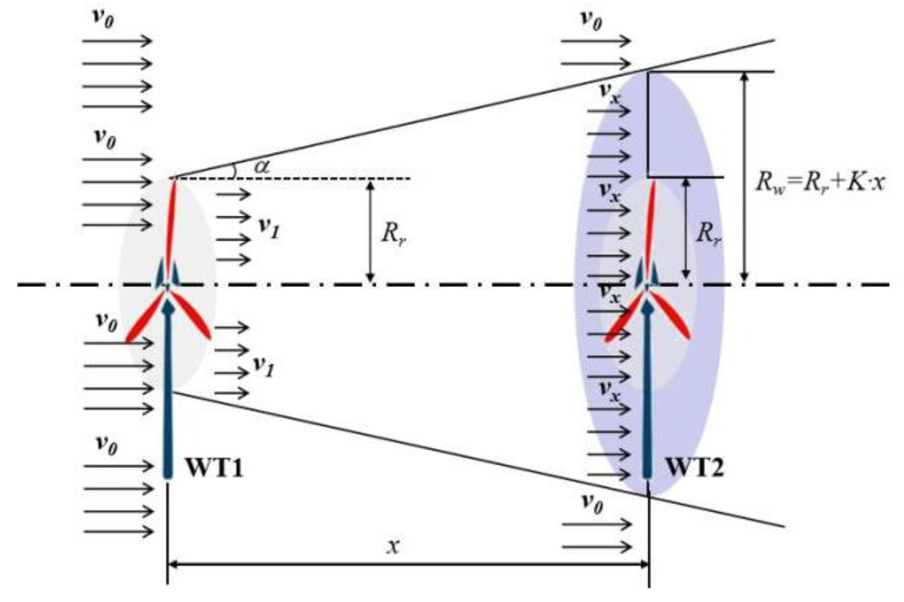
Figure 1. Schematic of Jensen’s wake model [26].
Energies 12 02482 g001
Figure 2. Wind shear.
Energies 12 02482 g002
Figure 3. Illustration of WTs’ wake on a flat area.
Energies 12 02482 g003
Figure 4. Illustration of WTs’ wake over a hill with gentle gradient.
Energies 12 02482 g004
Figure 5. Illustration of WTs’ wake over a hill with moderate gradient.
Energies 12 02482 g005
Figure 6. Two scenarios of wake overlap for a hilly WF.
Energies 12 02482 g006
Figure 7. Illustration of WTs’ wake over a hill with steep gradient.
Energies 12 02482 g007
Figure 8. Flowchart of the implementation of the power calculation function.
Energies 12 02482 g008
Figure 9. Simulation results of the WF power curve functions with different slopes.
Energies 12 02482 g009
Figure 10. Comparisons of the proposed model and Monte Carlo method with different slopes. (a) sample size = 100, s = 0; (b) sample size = 50,000, s = 0; (c) sample size = 100, s = 0.05; (d) sample size = 50,000, s = 0.05; (e) sample size = 100, s = 0.12; (f) sample size = 50,000, s = 0.12.
Energies 12 02482 g010
Table 1. Parameters of the simulation cases.
CtKRr [m]drow [m]Pr [kW]Pip [kW]vip [m/s]sv [kW·s·m−1]z0 [m]zref [m]
0.20.0754040020001091.29.37313.75140.310