Abstract
Train operation strategy optimization is a multi-objective optimization problem affected by multiple conditions and parameters, and it is difficult to solve it by using general optimization methods. In this paper, the parallel structure and double-population strategy are used to improve the general optimization algorithm. One population evolves by genetic algorithm (GA), and the other population evolves by particle swarm optimization (PSO). In order to make these two populations complement each other, an immigrant strategy is proposed, which can give full play to the overall advantages of parallel structure. In addition, GA and PSO is also improved, respectively. For GA, its convergence speed is improved by adjusting the selection pressure adaptively based on the current iteration number. Elite retention strategy (ERS) is introduced into GA, so that the best individual in each iteration can be saved and enter the next iteration process. In addition, the opposition-based learning (OBL) can produce the opposition population to maintain the diversity of the population and avoid the algorithm falling into local convergence as much as possible. For PSO, linear decreasing inertia weight (LDIW) is presented to better balance the global search ability and local search ability. Both MATLAB simulation results and hardware-in-the-loop (HIL) simulation results show that the proposed double-population genetic particle swarm optimization (DP-GAPSO) algorithm can solve the train operation strategy optimization problem quickly and effectively.
1. Introduction
The train operation system is a complex multi-objective nonlinear system, which needs to take into account multiple performance indicators such as safety, punctuality, energy saving, accurate parking and comfort [1,2,3]. At the same time, the train is restricted by a variety of constraints in the operating process, and it has a lot of uncertainty [4,5,6]. Therefore, how to use optimization methods to solve the train operation strategy is a hot issue in train research. At present, many intelligent optimization algorithms and their improved algorithms have been applied in train operation strategy optimization, such as genetic algorithm (GA), particle swarm optimization (PSO), simulated annealing (SA) algorithm, differential evolution (DE) algorithm, hybrid evolutionary algorithm and so on. Wang et al. [7] use GA with global search to optimize the speed curve of automatic train operation (ATO) to obtain an accurate train control sequence, which satisfies the speed protection index, punctuality index, accurate parking index, comfort index and energy saving index. The authors in [8], aiming at the ATO system, adopt the multi-objective optimization strategy of GA to optimize from five aspects: safety, accurate parking, punctuality, energy saving and comfort. In addition, the penalty function is added to the fitness function to improve the convergence speed of GA. Rong et al. [9] use PSO to solve the multi-objective optimization model of train operating process. Meanwhile, to solve the problem that the basic PSO are easily trapped into the local optimum in the late evolution period, the acceleration coefficient of PSO is improved. Shangguan et al. [10] propose a hybrid evolutionary algorithm based on DE and SA to solve the multi-objective optimization model for the speed trajectory to obtain an optimal velocity trajectory searching strategy.
The authors in [7,8,9,10] have achieved good results in the multi-objective optimization of train operation strategy through some common optimization algorithms, and one common feature of these algorithms is that the single population search method is used for the optimal solution. If the single population search strategy is extended to the multi-population search strategy, better optimization effect may be obtained. Therefore, many researchers have begun to study multi-population optimization algorithms in depth. Youneng et al. [11] propose a multi-population genetic algorithm (MPGA) to reduce the traction energy by optimizing the train operation for multiple interstations, and this method can get a better energy-efficient driving strategy. Zhou et al. [12] use the multi-objective multi-population ant colony optimization algorithm for continuous domain to solve the economic emission dispatch problem, and the pheromone structure of ant colony is reconstructed, which extends the original single-target method to the multi-target region. To overcome the premature convergence problem, the multi-population ant colony with different search range and speed is also proposed. Aiming at the problem of constrained optimization, Xu et al. [13] introduce a new method combining adaptive DE with multi-population mutation operators. In the process of mutation, the external population is combined with the main population to produce the evolutionary direction towards the optimal region. In addition, the new method can adaptively adjust DE’s control parameters according to the previous statistical information. Wang et al. [14] propose an adaptive multi-population optimization method for multi-objective optimization problem. In addition, this method combines PSO with DE to guide the exploitation of Pareto optimal solutions.
Based on the research results of literature [11,12,13,14], in this paper, a DP-GAPSO algorithm is proposed for the multi-objective optimization of train operation strategy, which can make up for the lack of a single population, a single method [15,16]. One population evolves by using GA, and the other population evolves by using PSO. In addition, the two branched populations adopt parallel structure to participate in evolution simultaneously [17,18]. Parallel structure refers to the fact that multiple tasks are not prioritized and can be carried out simultaneously to reduce the waiting time of the single task [19]. On the one hand, it can reduce the evolution time of the whole population, and, on the other hand, it simultaneously makes the two populations produce new individuals for further operation. To make the two populations complement each other, an immigrant strategy is proposed to exchange some good individuals between two populations, which can give full play to the overall advantages of parallel structure. In addition, GA and PSO are improved, respectively called IGA and IPSO, to achieve better optimization effect. For GA, individuals are selected by adjusting the selection pressure adaptively based on the current iteration number to improve the convergence speed. In order to prevent the destruction of the best individual in each iteration, elite retention strategy (ERS) is introduced into GA, which makes an important contribution to the convergence of the algorithm. The concept of opposition-based learning (OBL) was proposed by Tizhoosh in 2005 [20], who pointed out that the opposition solution was nearly 50% more likely to approach the optimal solution than the current solution. Therefore, GA uses the general dynamic OBL (which is a type of OBL) to generate opposition population. Then, the good individuals are selected from the current population and opposition population to form a temporary population to participate in next generation evolution, which expands the search area of the population. For PSO, the inertia weight determines the ability of the particle to inherit its previous velocity. Shi [21] first introduced the inertia weight into PSO. He also pointed out that a larger inertia weight was beneficial to global search, while a smaller inertia weight was more beneficial to local search. Thus, linear decreasing inertia weight (LDIW) is adopted to balance the global search ability and local search ability of PSO, which can improve the convergence speed of PSO.
In addition, the train operation strategy optimization should also take into account the eco-driving design in railways. Fernández-Rodríguez et al. [22] propose a real-time multi-objective optimization algorithm by means of fuzzy numbers to model the uncertainty of manual driving, considering the interference of delay. When a delay occurs, the system recalculates an optimal driving to reduce energy consumption. Aiming at the optimal energy-saving driving strategy of the train, Albrecht et al. [23] adopted a fast and effective numerical algorithm to solve the problem of the local energy minimization, so as to find the best switching point. The authors in [24] propose a robust and efficient method for designing velocity profile in the ATO equipment of the metro is proposed, which involves two objectives: running time and energy consumption. In addition, PSO is used to optimize the multi-objective model to minimize the total energy consumption. Bocharnikov et al. [25] design a fitness function with variable weight, and find the qualitative and quantitative effects of acceleration and braking rates on train energy saving by using genetic search method. The optimal train track is determined by using the fitness function. Lu et al. [26] propose a distance-based train track search model, which is optimized by various optimization algorithms. The results show that the ant colony algorithm achieves a good balance between stability and energy saving effect.
In order to verify that DP-GAPSO has better optimization performance for the multi-objective optimization of train operation strategy, three intervals of Rail transit line 12 and Jinpu line 1 in Dalian, China are selected for simulation test. Both MATLAB simulation and hardware-in-the-loop (HIL) simulation results show that, compared with IGA and IPSO, the multiple performance indexes obtained by DP-GAPSO have been improved to a considerable extent. Therefore, DP-GAPSO has better optimization performance.
2. Problem Description of Train Operation
Classic setup of discrete actions of train operation includes the full traction condition, constant speed condition, coasting condition and full braking condition as follows:
where the constant speed condition includes partial traction and partial braking, and the coasting condition means that the train exerts neither traction nor braking force.
A scientific research team at Beijing Jiaotong university in China has also proposed another setup of discrete actions of train operation according to the handle position of the train. Different handle positions correspond to different traction or braking forces. For example, the handle position of the train can be divided as follows:
where the maximum handle position is 4. The ratio of the current handle position to the maximum handle position is multiplied by the maximum traction or braking force to obtain the current traction or braking force.
Finally, we choose the classic setup of discrete actions of train operation () to study the train operation strategy. When the train runs in the same interval, the results obtained by using different combinations of operating conditions are also different. In this paper, we take the switching positions of the operating conditions and the corresponding operating conditions of the train as decision variables.
2.1. Safety Protection Curve
There are multiple speed limit sub-intervals in the train operating interval, and the speed of the train must be kept below the speed limit. The speed limit sub-intervals are divided into three cases: the speed constant limit sub-interval, the speed limit falling sub-interval and the speed limit rising sub-interval. These three cases are dealt with as follows:
- Speed constant limit sub-intervalAs shown in Figure 1a, in the constant speed limit sub-interval, when the actual running speed of the train is greater than or equal to the speed limit, the switching point of constant speed condition is inserted into the train control sequence to make the train maintain a constant running speed under the speed limit. In addition, this constant running speed curve is the safety protection curve.
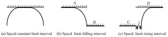 Figure 1. The processing of three speed limit sub-intervals: (a) Speed constant limit interval; (b) Speed limit falling interval; (c) Speed limit rising interval.
 - Speed limit falling sub-intervalIn the speed limit falling sub-interval, it is necessary to ensure that the train enters the low speed limit area at a speed which is less than the speed limit, so the train needs to brake and slow down in advance. As shown in Figure 1b, from the beginning point of the speed limiting section B, the reverse calculation is carried out under the full braking condition until the speed of the train equals the speed limit of the section A. By this reverse calculation method, the braking curve from the speed limiting section A to the speed limiting section B can be obtained, which is also called the safety protection curve.
- Speed limit rising sub-intervalAs shown in Figure 1c, l represents the length of the train. When the train enters the speed limit section D from the speed limit section C, it is necessary to ensure that the speed of the back for the train is below the speed limit of the section C. Therefore, the train cannot be accelerated immediately when its head leaves the speed limit section C. When the rear part of the train leaves the speed limit section C, the train accelerates under the full traction condition until the speed of the train equals the speed limit of the section D. By this method, the traction curve from the speed limiting section C to the speed limiting section D can be obtained, which is also called the safety protection curve.
The multi-segment safety protection curves can be obtained by preprocessing the whole operating interval according to the above three cases. These safety protection curves can be connected to obtain the safety protection curve of the whole operating interval. In the simulation operation, when the running speed of the train is greater than or equal to the speed of the safety protection curve, it is switched to the protection curve condition. Then, the train runs in accordance with the safety protection’s curve until the operating speed is lower than the protection curve, and the original condition of the train is restored. As shown in Figure 2, when the train reaches point A and point C, it switches to the condition of the safety protection curve. When the train reaches point B and point D, it will return to the original operating condition.
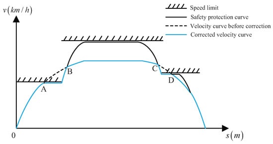
Figure 2.
The safety protection curve of the whole operating interval.
2.2. Initialization Settings for Operating Conditions
When the intelligent optimization algorithm is used to solve the optimal control sequence of train, there will be a lot of infeasible solutions if the train operating conditions are randomly generated within the entire running interval. In order to improve the efficiency of the algorithm, the ramps in entire running interval can be divided into the following three cases according to the forced condition of the train on the ramp.
- Case1:When the train is in the coasting condition (the train exerts neither traction nor braking force), the ramp in which the train still gets the same acceleration as the driving direction is called the big downhill.
- Case2:When the train is in the full traction condition, the ramp in which the train still slows down is called the big uphill.
- Case3:The remaining ramps except for case 1 and case 2 are continuous ramps.
According to these three cases, the entire interval can be divided into multiple sub-intervals. As you can see in Figure 3, for each sub-interval, its starting point is the beginning position of the big uphill or the continuous ramp, its middle point is the beginning position of the big downhill, and its end point is the end position of the big downhill. In Figure 3, the operating conditions within a sub-interval is set as . The switching point of the full traction condition (1) is the starting point of the sub-interval, as shown in Figure 3. The setting range of the switching point for the constant speed condition (0.5) is from the switching point of the previous full traction condition (1) to the middle point of the sub-interval, as shown 1 () in Figure 3. The setting range of the switching point for the coasting condition (0) is from the switching point of the previous constant speed condition (0.5) to the end point of the sub-interval, as shown 2 () in Figure 3. The full braking condition (−1) is inserted when the train running curve hits the safety protection curve. The train control sequence of the entire interval is the combination of the operating conditions of all the sub-intervals.
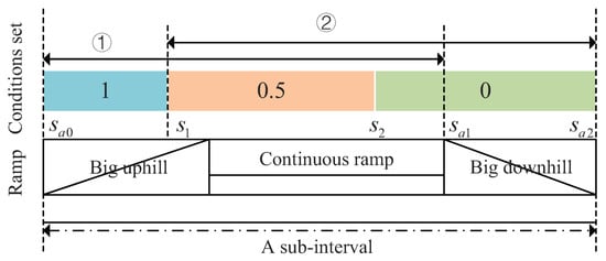
Figure 3.
Initialization settings of the operating conditions for the sub-interval.
3. Multi-Objective Optimization Model for the Train Operating Strategy
The train operating strategy optimization is a complex optimization problem that needs to meet multiple performance indexes such as energy saving, comfort level and punctuality at the same time [27,28]. The model for each performance index is as follows.
- The model of energy consumption for train operation strategy optimization iswhere is the energy consumed by the urban rail train; f and b are the traction force and braking force; A is the auxiliary power of the urban rail train; is the actual running time of the urban rail train between stations; is the conversion factor that converts electrical energy into mechanical energy during the urban rail train pulling; and is the conversion factor that converts mechanical energy into electrical energy during the urban rail train braking.
- The model of comfort index for train operation strategy optimization iswhere is passengers’ comfort level, which is generally reflected by the variation of acceleration of the train; is the rate of change of acceleration, also called . When is smaller, the passenger feels more comfortable. Research shows that the value of should be kept below 1.5 m/s. In order to simplify the calculation, the above model is improved as follows:where is expressed by the sum of the absolute value of the difference in acceleration of the two adjacent time steps; and are the two accelerations at the ith and th time steps, respectively.
- The model of punctuality index for train operation strategy optimization iswhere is the absolute value of the difference between the actual running time and the prescribed running time; is the speed of the train at the th time step; T is the prescribed time and is the actual running time between two stations.
Combined with the established performance indexes and multi-objective optimization theory, the multi-objective optimization model for train operating strategy is built as follows:
where Z is the multi-objective optimization model for train operating strategy; M is the mass of the train; u is the control sequence of the train; is the actual traction of the urban rail train, which is determined by u and the actual running speed v of the urban rail train; is the braking force of the urban rail train, which is determined by u and v; S is the distance between two given stations; is the speed limit of train operation; and is the actual running distance of the train between the two given stations. In general, the error between and S cannot exceed 30 cm, which can make passengers get on the train. is the running resistance of train, including basic resistance (frictional resistance and air resistance), additional resistance of ramp, additional resistance of curve and additional resistance of tunnel, as follows:
where is the running resistance of train; is the basic resistance of train; are empirical constants related to the train; v is the speed of the train; is additional resistance of ramp per unit weight; i is the slope, and its unit is ‰; Re3 is the additional resistance of curve; R is the radius of the track curve; L is the length of the train; Lr is the length at which the train overlaps the track curve; Re4 is additional resistance of tunnel; Ls is the length of the tunnel.
In addition, the multi-objective optimization problem for the train operating strategy can be transformed into the single-objective problem by the linear weighting method [29] as follows:
where f is the target function; , and are the weight coefficients of the three optimization indexes ().
To obtain the weight of each index more accurately, linear combination weights based on entropy (LCWBE) is used, which is both subjectivity and objectivity [30,31]. The steps of LCWBE is as follows.
For n given evaluation objects and m evaluation indexes, the evaluation matrix can be constructed as
Then, Equation (12) is normalized to obtain
In addition, the best evaluation object is an m-dimensional vector whose components are all 1. The experienced persons give l weight vectors () of evaluation indexes. The kth weight vector is , and it satisfies
is the weight vector obtained by the linear combination of (), and is
where is the linear combination coefficient and it satisfies
The generalized distance between the ith evaluation object and the best evaluation object is
Since the combination coefficient has uncertainty, the uncertainty can be expressed by Shannon information entropy [32] as follows:
Before solving the linear combination weight vector , it is necessary to determine the appropriate combination coefficient . On the one hand, the sum of the generalized distances between all evaluation objects and the best evaluation object should be minimized as follows:
On the other hand, the uncertainty of the combination coefficient should be eliminated as far as possible. According to Jaynes maximum entropy principle [33], the weight coefficient should make Shannon entropy maximum that is
Since it is a multi-objective optimization problem to solve the linear combination weight vector , it is converted to the single objective optimization as follows:
where is the balance coefficient between the two objectives, and it is set to 0.8.
It is verified that the above single-objective optimization problem has a unique solution, and the solution is
where .
Train operation strategy optimization has three optimization indexes (). In this paper, we select 10 objects () and three weight vectors of optimization indexes given by the experienced persons (). After the calculation of LCWBE, the weights of the three optimization indexes are 0.5124, 0.2854, 0.2022, respectively.
4. Train Operation Strategy Optimization Based on DM-GAPSO
Aiming at the problem of the train operation strategy optimization, DM-GAPSO which combines IGA with IPSO is proposed. This method makes up the deficiency of single population, and has obvious improvement in search speed and optimization effect.
4.1. IGA
The variables involved in the train operation strategy optimization is large, so it is difficult to find the optimal solution. GA is a kind of random search algorithm, including coding, crossover, selection, mutation operations [34], and it is good at solving such problem. Therefore, one population of DM-GAPSO evolves by GA, and GA is further improved. The detailed design of IGA is given below.
4.1.1. Code Design
By coding, the solution space of train operating strategy is transformed into the search space which can be processed by GA. The solution of train operation strategy optimization is the train control sequence, including the operating conditions and the switching positions of operating conditions. For the optimization of train operation strategy, the real number code is more effective than binary code and Gray code, which can directly use variables to code and facilitate the processing of large space search. In addition, real number coding eliminates the individual decoding process, which avoids data type conversion and improves the accuracy of solution. Therefore, real number coding is adopted in this paper. The chromosome in GA is the train control sequence u. To describe the train control sequence u more clearly, take Figure 4 for example.
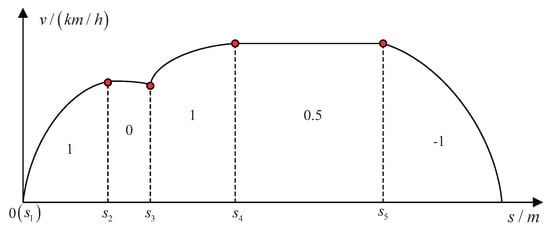
Figure 4.
Schematic diagram of the train control sequence.
As shown in Figure 4, the train control sequence u is coded as that is, a chromosome. represents a gene in the chromosome. For a given interval, the number of its genes cannot be changed once a chromosome is determined.
4.1.2. Fitness Function
Fitness function is the only basis of natural evolutionary selection, and the target function can be converted into a fitness function according to certain conversion rules. The greater the fitness value, the better the individual. The train operation strategy optimization is a problem of finding the minimum value, so the reciprocal of the target function can be used as the fitness function as follows:
where is the fitness function; is the target function; u is the train control sequence.
4.1.3. Select Operation
The linear sorting method based on adaptive change of selection pressure is used for a selection operator [34]. Firstly, all chromosomes in the population are sorted from largest to smallest according to their fitness function values, and the sorted chromosomes are shown in Equation (24). Then, each chromosome in the population is assigned a selected expected value p as follows:
where U is a population; n is the population size; is the jth chromosome (); is a parameter associated with selection pressure; when , the selection pressure is maximum, and the probability that the worst individual survives is 0. When , the selection pressure is the minimum, and all the individuals of parent population are randomly selected.
According to the number of iterations, the selection pressure can be adjusted adaptively to select the offspring individuals. At the early stage of the iteration, the individual differences in the population are large, so the selection pressure is lower to avoid the loss of population diversity. At the later stage of the iteration, the individual differences in the population become smaller, so the selection pressure is higher to find the optimal solution. The selection pressure increases as the number of the iterations increases as follows:
where k represents the current iterative number; is the maximum iterative number. The selection pressure is inversely proportional to .
After the linear sorting, the chromosomes in the parent population need to be selected in the offspring population by roulette wheel selection, as shown in Figure 5.
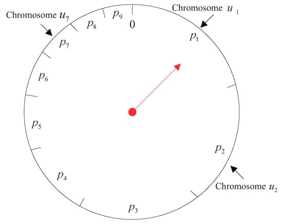
Figure 5.
The diagram of the roulette selection.
In Figure 5, taking nine chromosomes for example, the pointer on the wheel turns randomly to generate a random number a between 0 and 1. If , the chromosome is selected. The wheel needs to be turned nine times to get nine chromosomes.
4.1.4. Crossover Operation
The three-point crossover method is adopted for the crossover operation [35]. Two chromosomes are selected from the current population, and a number is randomly generated between 0 and 1. If the random number is less than the crossover probability , the selected two chromosomes performs the crossover operation. When performing the crossover operation, three crossover points are randomly generated. At this time, for the selected two chromosomes, the train operating conditions at these three crossover points are exchanged with each other, and the switching positions of operating conditions adopts the arithmetic crossover method to improve the diversity of the population as follows:
where ; ; and are the switching positions of the train operating conditions at the ith crossover point for the selected two chromosomes before performing the crossover operation; and are the switching positions of the train operating conditions at the ith crossover point for the selected two chromosomes after performing the crossover operation.
4.1.5. Mutation Operation
The crossover operation of chromosomes determines the global search ability of GA, and it can make local adjustment to the crossed chromosomes. In this paper, we adopt the probability mutation method [36]. First, a number is randomly generated between 0 and 1. If the random number is less than the mutation probability , the chromosome performs mutation operation. At the time, two mutation points are randomly generated, and the operating condition of each mutation point is randomly replaced by one of except the condition of the mutation point itself.
4.1.6. ERS
ERS: the individual with the highest fitness value in the current population does not participate in selection, crossover and mutation operation, and it is used to replace the individual with the lowest fitness value in the population produced by selection, crossover and mutation operations. GA adopts ERS, so that the best individual in each iteration can be saved and enter the next process.
is the optimal individual in the population of the ith generation, and is the new population of the th generation. If there is no better individual in than , then is added to as the th individual in , where n is the population size. In order to keep the population size unchanged, if the optimal individual is added to the new generation population, the individual with the smallest fitness value in the new generation population will be eliminated. Therefore, ERS can help excellent individuals avoid the damage caused by unnecessary crossover and mutation operations, which makes an important contribution to the convergence of the algorithm.
4.1.7. OBL
The concept of OBL was proposed by Tizhoosh in 2005, who pointed out that the opposition solution was nearly 50% more likely to approach the optimal solution than the current solution [20]. OBL is an effective method to improve the searching ability of random search algorithm. GA adopts general dynamic OBL (which is a type of OBL), which is defined as follows.
Let a feasible solution in M-dimensional search space be , which is defined as
The opposition solution of the feasible solution is
where ; and are the minimum and maximum values in the j dimension for the search space of the current population as follows:
where is the set of all values in the jth dimension for all individuals of the current population.
As shown in Figure 6, the general dynamic OBL is used to generate opposition population, and good individuals are selected from the current population and opposition population to form a temporary population, whose size is the same as the current population size. General dynamic OBL not only expands the search scope of the population, but also avoids invalid search. Therefore, OBL can drive the solutions obtained by GA as close to the global optima as possible.
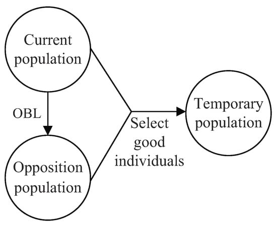
Figure 6.
General dynamic opposition-based learning (OBL).
The flow chart of IGA is shown in Figure 7.
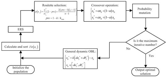
Figure 7.
The flow chart of improved genetic algorithm (IGA).
4.2. IPSO
PSO was proposed in 1995 by Eberhart and Kennedy, and it is a random search algorithm based on group cooperation developed by simulating the foraging behavior of birds [37]. Compared with GA, the optimization rules of PSO are simpler, without crossover and mutation operations of GA, and it seeks the global optimal solution by following the currently searched optimal value. PSO has attracted academic attention because of its advantages such as easy implementation and fast convergence. Therefore, another population of DM-GAPSO evolves by PSO, and PSO is further improved. The detailed design of IPSO is given below.
In a D-dimensional search space, n particles form a population X as follows:
where the ith particle in X represents a D-dimensional vector , and it also is a position in the D-dimensional search space.
The velocity of the ith particle is
The individual extreme value of the ith particle is
The global extreme value of the population is
In each iteration, each particle updates its speed and position through and , as shown in Equation (35):
where is the inertia weight; ; ; k is the current iterative number; is the velocity in the dth dimension of the ith particle; and are nonnegative constants (acceleration factors); and are random numbers between 0 and 1. To prevent particles from searching blindly, their position and velocity should be limited to a certain area ().
The inertia weight determines the ability of the particle to inherit its previous velocity. Shi first introduced the inertia weight into PSO, who also pointed out that a larger inertia weight is beneficial to global search, while a smaller inertia weight is more beneficial to local search [21]. Thus, LDIW is proposed to better balance the global search ability and local search ability of PSO as follows:
where is the initial inertia weight; is the inertia weight at the maximum iterative number; k is the current iteration number; is the maximum iterative number. It has been verified by many experiments that PSO has better optimization performance when and .
In the iterative process, the inertia weight decreases from 0.9 to 0.4. At the beginning of iteration, the larger inertia weight keeps PSO strong global search capability. At the end of the iteration, the smaller inertia weight is beneficial to the local search more accurately. The inertial weight is a dynamically changing value.
In addition, IPSO also adopts OBL strategy which is similar to IGA. In addition, the flow chart of IPSO is shown in Figure 8.
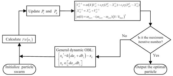
Figure 8.
The flow chart of improved particle swarm optimization (IPSO).
4.3. DM-GAPSO Based on IGA and IPSO
4.3.1. DM-GAPSO
Aiming at the problem of the train operation strategy optimization, the parallel structure and double-population strategy are adopted to construct DM-GAPSO based on IGA and IPSO [38,39,40]. As shown in Figure 9, after calculating the fitness values of all chromosomes in the initial population, DM-GAPSO distributes all chromosomes in the initial population equally to two parallel populations according to the size of their fitness values.
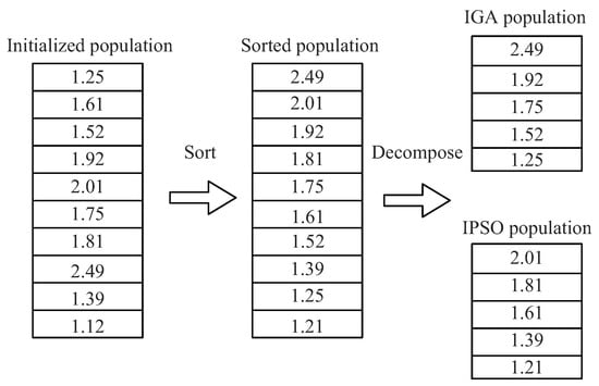
Figure 9.
Parallel decomposition of the initial population.
For DM-GAPSO, one branch population adopts IGA to evolve, the other adopts IPSO to evolve. Two branch populations exchange good individuals through the immigrant strategy, which will be explained in detail later. These exchanged individuals as excellent exotic species can effectively improve the individual diversity of the population. The basic flow of DM-GAPSO is as follows:
- Step 1: Initialize the population.
- Step 2: The fitness value of each chromosome in the initial population is calculated, and all individuals are evenly distributed into two parallel populations after sequencing.
- Step 3: The two parallel populations evolve according to IGA and IPSO, respectively.
- Step 4: The immigrant strategy is used to judge the two parallel populations. If the judgment result meets the immigration conditions, the immigration operation shall be carried out.
- Step 5: Judge whether the current process meets the termination condition. If so, terminate the process; if not, switch to step 3.
The flow chart of DM-GAPSO is shown in Figure 10.
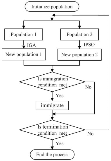
Figure 10.
The flow chart of DM-GAPSO.
4.3.2. Immigrant Strategy
In order to make the two populations complement each other, an immigrant strategy is proposed, which can take advantage of the whole parallel architecture. As shown in Figure 11, the immigrant strategy is that some good individuals are exchanged between two parallel branch populations after a certain iterative number that is the immigrant frequency f. The exchanged individuals, as exotic good individuals, can make up for the lack of population diversity in the late evolutionary period. The implementation of immigration strategy needs to design two important parameters, namely, f and immigrant number N. If f is too small, when one branch population falls into local optimum, the other branch population is also prone to fall into local optimality, which cannot effectively play the mutual promotion between the two branch populations. N is the number of good individuals to be exchanged in each immigrant process. If N is too large, the chromosomes of the two branch populations will tend to be the same, which also makes the algorithm trap in the local optimum.
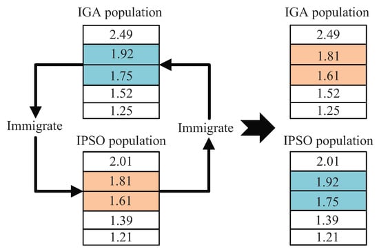
Figure 11.
The immigrant process of two parallel branch populations.
Aiming at the problem of the train operation strategy optimization, the different f and N are used for experimental analysis, and the fitness function values of the optimal solutions are obtained as shown in Table 1. In addition, the population size is 100 and the branch population size is 50. Since only a small number of good individuals are immigrated, the range of N is set as 1–6, and the range of f is set as 1–9.

Table 1.
The fitness values of the optimal solutions obtained by using different immigrant strategies.
As can be seen from the data in Table 1, when and , the fitness value (2.49) of the optimal solution is the highest. It indicates that, when and , DM-GAPSO has better optimization effect. Therefore, in this paper, we set f and N as 4 and 2.
5. Results and Discussion
5.1. Experimental Relevant Data
In order to verify that DP-GAPSO has better optimization performance for the multi-objective optimization of train operation strategy, two trains of Rail transit line 12 and Jinpu line 1 in Dalian, China are selected as research objects. For the train of Rail transit line 12, the interval from New Port in Lvshun to Tieshan town is selected for simulation, with the length of 2.94 km. For the train of Jinpu line 1, the two intervals from Dalian North Station to Houyan and from Houyan to Qianguan are selected for simulation, with the length of 3.21 km and the length of 2.91 km. The basic attributes of the two trains are shown in Table 2 and Table 3. The ramp parameters and speed limit for the three intervals are shown in Table 4, Table 5, Table 6, Table 7, Table 8 and Table 9.
Table 2.
The attributes for the train of Rail transit line 12.
Table 3.
The attributes for the train of Jinpu line 1.
Table 4.
The ramp parameters from New Port in Lvshun to Tieshan town.
Table 5.
The speed limit from New Port in Lvshun to Tieshan town.
Table 6.
The ramp parameters from Dalian North Station to Houyan.
Table 7.
The speed limit from Dalian North Station to Houyan.
Table 8.
The ramp parameters from Houyan to Qianguan.
Table 9.
The speed limit from Houyan to Qianguan.
5.2. MATLAB Simulation Results and Analysis
In the MATLAB (2016a, MathWorks, Natick, MA, US) simulation environment, based on two intervals for Rail transit line 12 and Jinpu line 1 in Dalian, China, DP-GAPSO, IGA and IPSO are used to solve the multi-objective optimization model of train operation strategy. For the interval from New Port in Lvshun to Tieshan town in Rail transit line 12, its preset time is 180 s. The speed distance curve of the train, the operating condition distance curve of the train (which is also the train control sequence), and the iterative convergence curve of three optimization indexes (which are energy consumption, comfort and punctuality) are shown in Figure 12, Figure 13 and Figure 14. The computation times for three optimization algorithms are shown in Table 10, and the optimization results obtained by three different optimization algorithms are shown in Table 11.
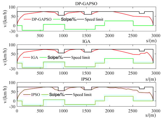
Figure 12.
The speed distance curve of the train from New Port in Lvshun to Tieshan town.
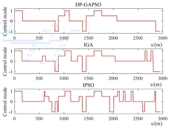
Figure 13.
The operating condition distance curve of the train from New Port in Lvshun to Tieshan town.
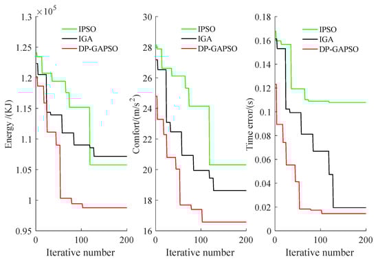
Figure 14.
The iterative convergence curve of three optimization indexes from New Port in Lvshun to Tieshan town.
Table 10.
The computation times for three optimization algorithms.
Table 11.
The optimization results obtained by the three optimization algorithms from New Port in Lvshun to Tieshan town.
In Figure 12, the speed distance curve obtained by DP-GAPSO is smoother, and DP-GAPSO makes the train maintain the appropriate speed more steadily, which can make passengers feel more comfortable. In Figure 13, for the train control sequence obtained by DP-GAPSO, it has a lower number of switching operation conditions, and the time taken in coasting condition and constant speed condition is relatively large. This train operating strategy helps avoid bumps and saves energy consumption. In Figure 14, compared with IGA and IPSO, the three optimization indexes obtained by DP-GAPSO have been improved to a considerable extent not only in the convergence speed but also in the optimization effect. In Table 10, the computation time for DP-GAPSO is the least. It indicates that DP-GAPSO improves the convergence speed. In Table 11, compared with IGA and IPSO, three optimization indexes of DP-GAPSO are all the best. Especially for energy consumption and comfort indexes, the energy consumption obtained by DP-GAPSO is 8.94% and 7.66% lower than that of IGA and IPSO, and the comfort level obtained by DP-GAPSO is 9.33% and 19.43% higher than that of IGA and IPSO.
For the interval from Dalian North Station to Houyan in Jinpu line 1, its preset time is 210 s. The speed distance curve of the train and the operating condition distance curve of the train are shown in Figure 15 and Figure 16. The optimization results obtained by three different optimization algorithms are shown in Table 12.
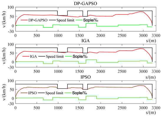
Figure 15.
The speed distance curve of the train from Dalian North Station to Houyan.
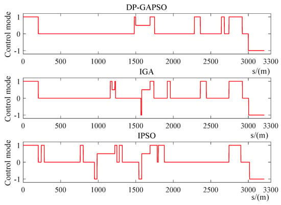
Figure 16.
The operating condition distance curve of the train from Dalian North Station to Houyan.
Table 12.
The optimization results obtained by three different optimization algorithms from Dalian North Station to Houyan.
In Figure 15 and Figure 16, DP-GAPSO enables the train to remain in coasting condition (0) for a long distance (202–1480 m), which can greatly reduce the energy consumption of the train. In addition, the number of switching operating conditions for the train control sequence obtained by DP-GAPSO are 12, which is a lot less than 16 of IGA and 20 of IPSO. This train control sequence greatly improves passengers’ comfort. In Table 12, compared with IGA and IPSO, the three optimization indexes obtained by DP-GAPSO are obviously improved.
Therefore, the simulation results verify that DP-GAPSO has better optimization performance for the multi-objective optimization of train operation strategy.
5.3. HIL Simulation Results and Analysis
MATLAB simulation is a pure simulation technology separated from the actual operation environment. To more effectively verify that DP-GAPSO has better optimization performance for the multi-objective optimization of train operation strategy, we also use dSPACE HIL simulation technology. In HIL simulation based on the half-physical environment of the train, dSPACE is the controlled object of ATO, namely the train model. Then, the train model that has been designed in Simulink is downloaded to dSPACE and connected with the real vehicle on-board controller (VOBC) through the real physical interface. In addition, PC is used to import the actual train line data into dSPACE, and the optimizer produces the ATO target speed curve according to the line information. The function of VOBC is to track the target speed curve of ATO as much as possible. In addition, the data of train operation can be directly observed by Control Desk (7.0, dSPACE, Paderborn, Germany), the software of dSPACE. When the control effect is not ideal, the control parameters can be modified online and in real time in the Control Desk to improve the control effect. HIL simulation has real on-board equipment, including sensors, optimizer, controller, conditioning circuit, signal processing unit and so on, as shown in Figure 17.
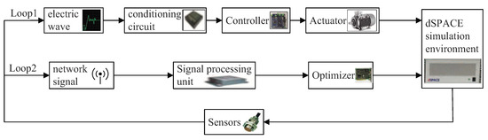
Figure 17.
Hardware-in-the-loop (HIL) simulation structure.
In Figure 17, the loop1 is “low-level control behavior loop”, and the loop2 is “high-level optimization strategy loop”. “Conditioning circuit” can regulate electrical signals accordingly; “Signal processing unit” can adjust the network signals accordingly; “Controller” can apply real-time instruction control of ATO according to the actual situation; “Optimizer” can produce ATO target speed curve; “Sensors” can feed some information such as speed, position and current back to the control system in real time. According to HIL simulation platform of the interval from Houyan to Qianguan in Jinpu line 1, these three optimization algorithms including DP-GAPSO, IGA and IPSO are written into the optimizer respectively to produce the target speed curves of ATO, and the model predictive control (MPC) algorithm is written into the controller to track the target speed curve. The preset time of the interval is 190 s. In HIL simulation, the optimization results obtained by three different algorithms are shown in Figure 18 and Figure 19 and Table 13. In Figure 18 and Figure 19, the regional options show that HIL is online, and the optimizer and controller are in working state. When “Profiles” is selected, the speed distance curve of the train is displayed, as shown in Figure 18. When the multi-option button is “(u, s)sequence”, the train control sequence can be displayed, as shown in Figure 19.
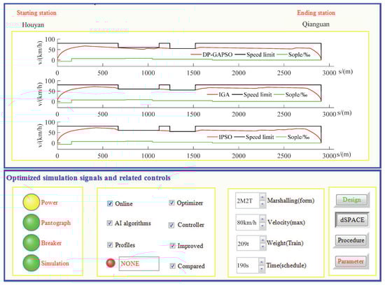
Figure 18.
The speed distance curve of the train from Houyan to Qianguan.
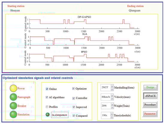
Figure 19.
The operating condition distance curve of the train from Houyan to Qianguan.
Table 13.
The simulation results obtained by three different algorithms from Houyan to Qianguan.
In Figure 18 and Figure 19, DP-GAPSO enables the train to reduce unnecessary braking conditions and to keep as much in coasting condition (0) as possible, which can significantly reduce energy consumption. The number of switching operating conditions for the train control sequence obtained by DP-GAPSO is also relatively small, which helps improve the comfort index. In Table 13, compared with IGA and IPSO, the energy consumption obtained by DP-GAPSO is 10.39% and 11.96% lower than that of IGA and IPSO, and the comfort level obtained by DP-GAPSO is 15.80% and 23.95% higher than that of IGA and IPSO. Thus, the two optimization indexes (energy consumption and comfort level) obtained by DP-GAPSO are obviously improved. However, the punctuality index obtained by DP-GAPSO is 0.0389 s, which is worse than IGA and IPSO. Because 0.0389 s is too small for the actual operation process of the train, its effect on the punctual arrival of trains can be ignored.
Therefore, HIL simulation results also verify that DP-GAPSO has better optimization performance for the multi-objective optimization of train operation strategy.
6. Conclusions
In this paper, taking energy saving, comfort and punctuality as optimization indexes, the multi-objective optimization model of train operation strategy is established, and the multi-objective optimization problem is transformed into the single-objective optimization problem by using a linear weighting method. In addition, LCWBE that takes account of both subjectivity and objectivity is used to obtain the weight of each index more accurately. Aiming at the multi-objective optimization of the train operation strategy, a DP-GAPSO algorithm is proposed to obtain the optimal operation strategy, which adopts a parallel structure and double-population optimization strategy. One population evolves by using GA, and the other population evolves by using PSO. To make these two populations complement each other, an immigrant strategy is proposed to exchange some good individuals between two populations, which can give full play to the overall advantages of parallel structure.
In addition, GA and PSO are improved, respectively. For GA, its convergence rate and optimization effect are improved by adjusting the selection pressure adaptively based on the current iteration number. ERS is introduced into the GA to avoid destroying the best individual in each iteration. In order to avoid the algorithm falling into local optimum as far as possible, OBL is used to generate the opposition population. In addition, the opposite population participates in evolution along with the current population. For PSO, LDIW is proposed to better balance the global search ability and local search ability, so that better optimization effect can be obtained. Simulation results show that DP-GAPSO has achieved good results for train operation strategy optimization.
However, the individual exchange strategy such as immigrant strategy between two parallel populations is not perfect, and this strategy is the focus of the double-population algorithm. Through the analysis and summary of a large number of experimental results, a more reasonable immigrant strategy may be obtained. Therefore, the further improvement of this strategy in the future can achieve better optimization results.
Author Contributions
Conceptualization, methodology and formal analysis were made by K.L. and X.W.; Data curation, writing—original draft preparation and writing—review and editing was made by K.L.; Resources, supervision and project administration were made by X.W. and Z.Q.
Funding
This research was supported by the National Natural Science Foundation of China (60574018).
Conflicts of Interest
The authors declare no conflict of interest.
References
- Gu, Q.; Tang, T.; Cao, F. Energy-Efficient Train Operation in Urban Rail Transit Using Real-Time Traffic Information. IEEE Trans. Intell. Transp. Syst. 2014, 15, 1216–1233. [Google Scholar] [CrossRef]
- Meng, J.; Xu, R.; Li, D. Combining the Matter-Element Model With the Associated Function of Performance Indices for Automatic Train Operation Algorithm. IEEE Trans. Intell. Transp. Syst. 2018, 99, 1–11. [Google Scholar] [CrossRef]
- Li, W.J.; Lei, N. An improved cellular automata model for train operation simulation with dynamic acceleration. Mod. Phys. Lett. B 2018, 32, 1850087. [Google Scholar] [CrossRef]
- Kunimatsu, T.; Hirai, C.; Tomii, N. Train timetable evaluation from the viewpoint of passengers by microsimulation of train operation and passenger flow. Electr. Eng. Jpn. 2012, 181, 51–62. [Google Scholar] [CrossRef]
- Wang, Z.; Ceder, A. Efficient design of freight train operation with double-hump yards. J. Oper. Res. Soc. 2017, 68, 1–20. [Google Scholar] [CrossRef]
- Gao, S.; Dong, H.; Ning, B. Adaptive fault-tolerant automatic train operation using RBF neural networks. Neural Comput. Appl. 2015, 26, 141–149. [Google Scholar] [CrossRef]
- Wang, G.; Xiao, S.; Chen, X. Application of Genetic Algorithm in Automatic Train Operation. Wirel. Pers. Commun. 2018, 102, 1695–1704. [Google Scholar] [CrossRef]
- Liang, Y.; Liu, H.; Qian, C. A Modified Genetic Algorithm for Multi-Objective Optimization on Running Curve of Automatic Train Operation System Using Penalty Function Method. Int. J. Intell. Transp. Syst. Res. 2019, 17, 74–87. [Google Scholar] [CrossRef]
- Rong, H.; Yu, C.Z. Multiple Objective of Train Operation Process Based on Modified Particle Swarm Optimization. Appl. Mech. Mater. 2014, 513–517, 2927–2930. [Google Scholar] [CrossRef]
- Shangguan, W.; Yan, X.H.; Cai, B.G. Multiobjective Optimization for Train Speed Trajectory in CTCS High-Speed Railway With Hybrid Evolutionary Algorithm. IEEE Trans. Intell. Transp. Syst. 2015, 16, 2215–2225. [Google Scholar] [CrossRef]
- Youneng, H.; Xiao, M.; Shuai, S. Optimization of Train Operation in Multiple Interstations with Multi-Population Genetic Algorithm. Energies 2015, 8, 14311–14329. [Google Scholar]
- Zhou, J.; Wang, C.; Li, Y. A multi-objective multi-population ant colony optimization for economic emission dispatch considering power system security. Appl. Math. Model. 2017, 45, 684–704. [Google Scholar] [CrossRef]
- Xu, B.; Tao, L.; Chen, X. Adaptive differential evolution with multi-population-based mutation operators for constrained optimization. Soft Comput. 2019, 23, 3423–3447. [Google Scholar] [CrossRef]
- Wang, H.; Fu, Y.; Huang, M. A hybrid evolutionary algorithm with adaptive multi-population strategy for multi-objective optimization problems. Soft Comput. 2017, 21, 5975–5987. [Google Scholar] [CrossRef]
- Ming, Z.; Ji, Z.; Yan, W. Artificial bee colony algorithm with dynamic multi-population. Mod. Phys. Lett. B 2017, 31, 1740087. [Google Scholar]
- Zhang, L.; Qin, Y.; Meng, X. MPSO-Based Model of Train Operation Adjustment. Procedia Eng. 2016, 137, 114–123. [Google Scholar] [CrossRef]
- Caraffini, F.; Neri, F.; Iacca, G.; Mol, A. Parallel memetic structures. Inf. Sci. 2013, 227, 60–82. [Google Scholar] [CrossRef]
- Habershon, S.; Harris, K.D.M.; Johnston, R.L. Development of a multipopulation parallel genetic algorithm for structure solution from powder diffraction data. J. Comput. Chem. 2010, 24, 1766–1774. [Google Scholar] [CrossRef]
- St-Gelais, R.; Zhu, L.; Fan, S. Near-field radiative heat transfer between parallel structures in the deep subwavelength regime. Nat. Nanotechnol. 2016, 11, 515–519. [Google Scholar] [CrossRef]
- Tizhoosh, H.R. Opposition-Based Learning: A New Scheme for Machine Intelligence. In Proceedings of the International Conference on Computational Intelligence for Modelling, Control & Automation, & International Conference on Intelligent Agents, Web Technologies & Internet Commerce, Vienna, Austria, 28–30 November 2005. [Google Scholar]
- Shi, Y. A Modified Particle Swarm Optimizer. In Proceedings of the 1998 IEEE International Conference on Evolutionary Computation Proceedings, Anchorage, AK, USA, 4–9 May 1998. [Google Scholar]
- Fernández-Rodríguez, A.; Fernandez-Cardador, A.; Cucala, A.P. Balancing energy consumption and risk of delay in high speed trains: A three-objective real-time eco-driving algorithm with fuzzy parameters. Transp. Res. Part C Emerg. Technol. 2018, 95, 652–678. [Google Scholar] [CrossRef]
- Albrecht, A.; Howlett, P.; Pudney, P.; Vu, X. Optimal train control: Analysis of a new local optimization principle. In Proceedings of the 2011 American Control Conference, San Francisco, CA, USA, 29 June–1 July 2011; pp. 1928–1933. [Google Scholar]
- Fernández-Rodríguez, A.; Fernandez-Cardador, A.; Cucala, A.P.; Dominguez, M.; Gonsalves, T. Design of Robust and Energy-Efficient ATO Speed Profiles of Metropolitan Lines Considering Train Load Variations and Delays. IEEE Trans. Intell. Transp. Syst. 2015, 16, 2061–2071. [Google Scholar] [CrossRef]
- Bocharnikov, Y.V.; Tobias, A.M.; Roberts, C.; Hillmansen, S.; Goodman, C.J. Optimal driving strategy for traction energy saving on DC suburban railways. IET Electr. Power Appl. 2007, 1, 675–682. [Google Scholar] [CrossRef]
- Lu, S.; Hillmansen, S.; Ho, T.K.; Roberts, C. Single-Train Trajectory Optimization. IEEE Trans. Intell. Transp. Syst. 2013, 14, 743–750. [Google Scholar] [CrossRef]
- Gu, Q.; Tao, T.; Fei, M. Energy-Efficient Train Tracking Operation Based on Multiple Optimization Models. IEEE Trans. Intell. Transp. Syst. 2016, 17, 882–892. [Google Scholar] [CrossRef]
- Miao, Z.; Wang, Y.; Shuai, S. A Short Turning Strategy for Train Scheduling Optimization in an Urban Rail Transit Line: The Case of Beijing Subway Line 4. J. Adv. Transp. 2018, 2018, 1–19. [Google Scholar]
- Ramanathan, R. ABC inventory classification with multiple-criteria using weighted linear optimization. Neural Comput. Appl. 2006, 33, 695–700. [Google Scholar] [CrossRef]
- Wang, S.L. A Novel Multi-Attribute Allocation Method Based on Entropy Principle. J. Softw. Eng. 2012, 6, 16–20. [Google Scholar] [CrossRef][Green Version]
- Rocha, L.C.S.; Paiva, A.P.D.; Balestrassi, P.P.; Severino, G.; Junior, P.R. Entropy-Based Weighting for Multiobjective Optimization: An Application on Vertical Turning. Math. Probl. Eng. 2015, 2015, 1–11. [Google Scholar] [CrossRef]
- Strait, B.J.; Dewey, T.G. The Shannon information entropy of protein sequences. Biophys. J. 1996, 71, 148–155. [Google Scholar] [CrossRef]
- Kaniadakis, G. Maximum entropy principle and power-law tailed distributions. Eur. Phys. J. B 2009, 70, 3–13. [Google Scholar] [CrossRef]
- AL-Madi, N.A.; Maria, K.A.; Maria, E.A.; AL-Madi, M.A. A structured-population human community based genetic algorithm (HCBGA) in a comparison with both the standard genetic algorithm (SGA) and the cellular genetic algorithm (CGA). ICIC Express Lett. 2018, 12, 1267–1275. [Google Scholar]
- Shigei, N.; Miyajima, H.; Ozono, H. Acceleration of Genetic Algorithm for Peak Power Reduction of OFDM Signal. IAENG Int. J. Comput. Sci. 2011, 38, 294–297. [Google Scholar]
- Serpell, M.; Smith, J.E. Self-Adaptation of Mutation Operator and Probability for Permutation Representations in Genetic Algorithms. Evolut. Comput. 2010, 18, 491–514. [Google Scholar] [CrossRef]
- Kennedy, J.; Eberhart, R. Particle swarm optimization. IEEE Int. Conf. Neural Netw. 2011, 4, 1942–1948. [Google Scholar]
- Hao, W.; Cai, W.; Wang, Y. Optimization of a hybrid ejector air conditioning system with PSOGA. Appl. Therm. Eng. 2017, 112, 1474–1486. [Google Scholar]
- Zhai, Z.; Martínez, J.O.; Lucas, N.M. A Mission Planning Approach for Precision Farming Systems Based on Multi-Objective Optimization. Sensors 2018, 18, 1795. [Google Scholar] [CrossRef]
- Agarwal, M.; Srivastava, G.M.S. Genetic Algorithm-Enabled Particle Swarm Optimization (PSOGA)-Based Task Scheduling in Cloud Computing Environment. Int. J. Inf. Technol. Decis. Mak. 2018, 17, 1237–1267. [Google Scholar] [CrossRef]


© 2019 by the authors. Licensee MDPI, Basel, Switzerland. This article is an open access article distributed under the terms and conditions of the Creative Commons Attribution (CC BY) license (http://creativecommons.org/licenses/by/4.0/).