Water Hammer Control Analysis of an Intelligent Surge Tank with Spring Self-Adaptive Auxiliary Control System

Abstract

The water hammer can cause great risks in water supply pipe systems. A surge tank is a kind of general water hammer control device. In order to improve the behavior of the surge tank, a self-adaptive auxiliary control (SAC) system was proposed in this paper. The system can optimize the response of the surge tank according to the transient pressure. The numerical model and the matched boundary conditions were established to simulate the improved surge tank and optimize the SAC system. Then, various transient responses were simulated by the proposed model with different parameters set. The proposed system is validated by comparing the water hammer process in a river-pipe-valve (RLV) system with and without SAC. The results show that the SAC can greatly improve the water hammer control of the pipeline and the water level oscillation of the surge tank. With the SAC system, the required vertical size of the surge tank can be significantly reduced with the desired water hammer control function.

1. Introduction

In pressured piping systems, the water hammer is an undesired hydraulic phenomenon with a rapid change in flow velocity and pressure [1]. It usually occurs with a valve shutdown and opening, a pump accident and start-up, or even a sudden depressurization of a pipeline system. The water hammer is common in pump rise systems [2,3,4,5], hydroelectric station systems [6,7,8], hydraulic conveying systems [9,10,11,12], and even in oil conveying fields [13,14] and so on. Unfortunately, water hammers can cause severe pressure and flow oscillations, along with cavitation, noise, and other hazards. In particular, the instantaneous positive and negative pressure generated by the water hammer is much greater than the normal operating pressure of the pipeline. The positive pressure can lead to valve damage and pipe burst, while the negative pressure can crush the pipe. In addition, the pressure and flow oscillations can also make the pump and water turbine unit out of control.

In order to eliminate and mitigate the hazards of water hammers, the prediction and prevention of water hammers has always been a common concern of engineers and researchers. Especially, the focus of attention is how to reduce the peak pressure and the trough pressure caused by water hammers. The main purpose is to reduce the amplitude and duration of the pressure oscillation of the water hammer. In other words, how to reduce the extreme high pressure and increase the extreme low pressure is very significant for water hammer protection. At present, the methods of reducing the water hammer mainly include optimizing operation mode and installing water hammer control equipment. The improvement of the valve closing rule and the coordinated operation of the system are common optimized operation methods [15,16,17,18]. However, optimized operations cannot always meet the requirements of water hammer control and sometimes protective devices are necessary to better control the water hammer. At present, there is various water hammer control equipment, including surge tanks, relief valves, air pressure vessels, and so on. In addition, with the development of related research, some new types of equipment have been proposed and applied [19,20,21,22]. Nevertheless, surge tanks are one of the most widely used water hammer protection devices. It is very popular in water conveyance systems, pump systems, and power station systems. There is a lot of research on surge tanks, but they are still being developed and improved. However, it is worth mentioning that the surge tank may experience large fluctuations in the water level in order to control the water hammer by absorbing and storing water. Therefore, it is necessary to have a sufficient section size and a vertical height. Consequently, surge tanks are often constrained by site and elevation, which severely limits the practical application of the surge tank. In particular, in a long-distance pipeline, the pressure peak may be higher than the ground elevation and the pressure trough may be lower than the pipeline elevation. When the section area of the surge tank is constrained, the water level fluctuation in the surge tank may be higher than the ground and lower than the installation elevation of pipeline. In this case, regular surge tanks are no longer applicable.

In order to solve this problem, this paper proposes a self-adaptive auxiliary control system. The system can reduce the water level fluctuation by setting the initial threshold and the elastic opening coefficient of the orifice. In fact, this kind of surge tank only takes effective work in the specific extreme conditions. Therefore, the improvement can be accessed by adjusting the work zone by setting the response threshold value. In the research, we proposed a self-adaptive auxiliary control (SAC) method to improve the surge tank. The improved surge tank doesn’t need to work when the pressure is in the tolerable zone. In other words, it only needs to work when the pressure exceeds the set range. For the same cross-sectional area, the maximum elevation required for the surge tank decreases while the minimum elevation required increases, as well as smaller surge tank heights that are applicative. In addition, in order to select the appropriate initial threshold and orifice elasticity coefficient, a multifactor optimization method is established. Fortunately, the proposed self-adaptive auxiliary control system can greatly improve the behavior of the surge tank. The results show that the optimized SAC can greatly reduce the amplitude and the height of water mass oscillation in the surge tank, as well as the extreme transient pressure and the duration of large amplitude oscillation in the pipeline.

2. Intelligent Surge Tank with Self-Adaptive Auxiliary Control (SAC)

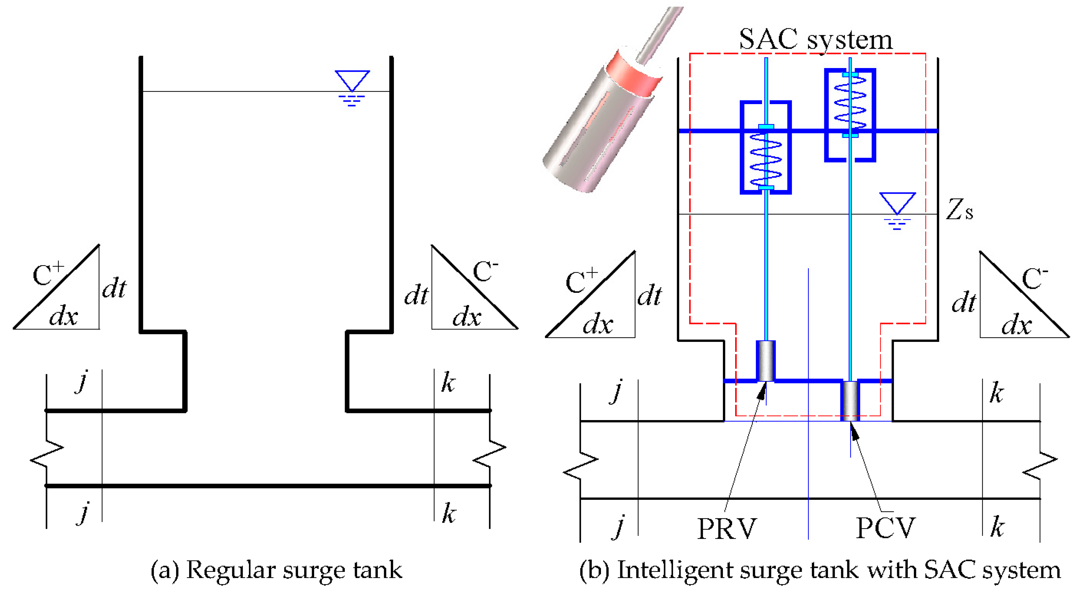
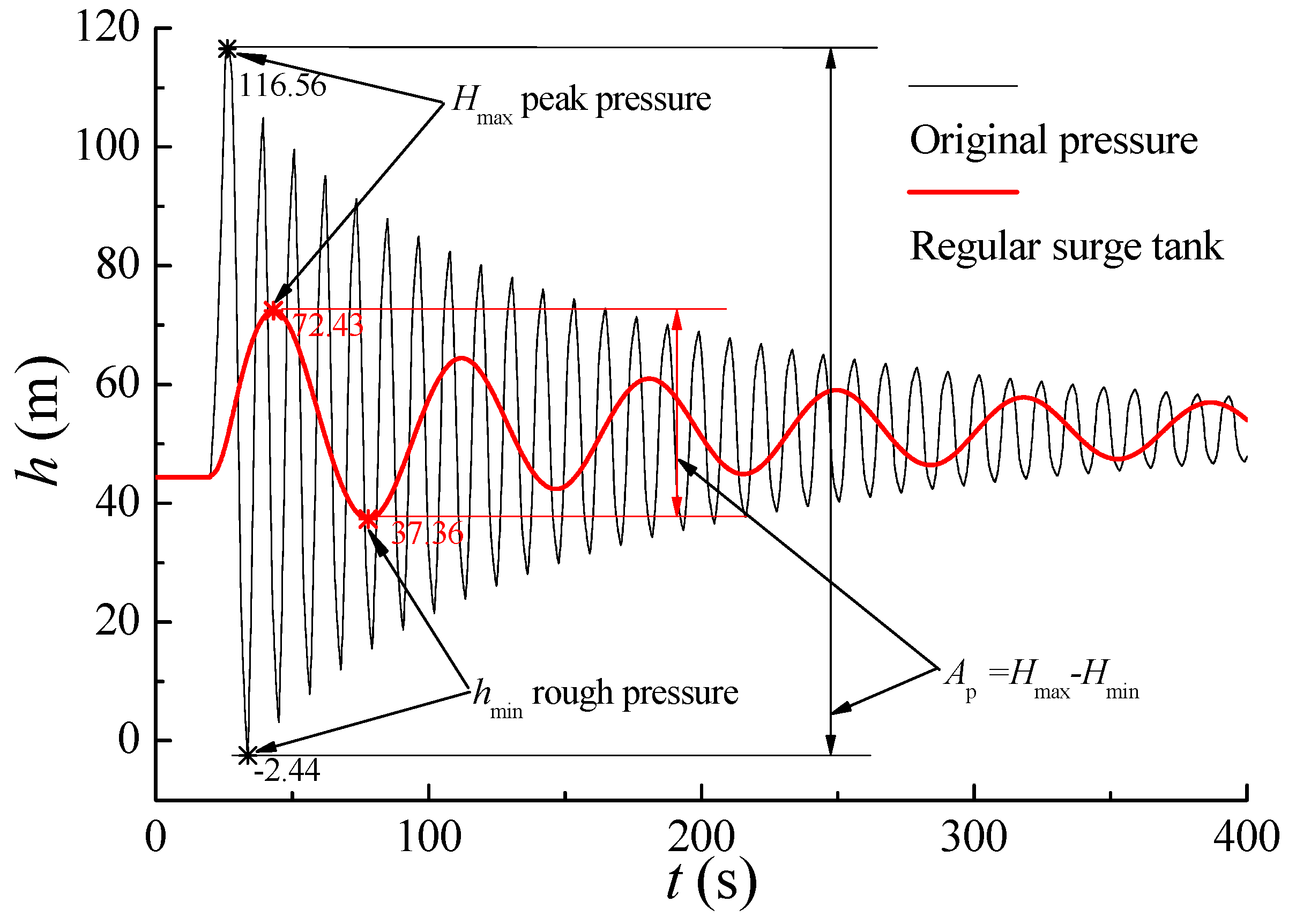
2.1. Basic Properties of a Regular Surge Tank

In order to illustrate the SAC proposed in this paper, the structure and function of the regular pressure surge tank are briefly described as the reference, and then the SAC is introduced and analyzed for comparison. Commonly, a surge tank is fixed in closed pipes to reduce the oscillations of transient pressure. Figure 1a shows a regular surge tank in a reservoir-pipe-valve (RPV) system. The water hammer occurs in the water supply pipe system when the valve is closed suddenly. During the transient process, the surge tank will absorb water from the main pipe to restrain the raising of the pressure. On the contrary, the surge tank will compensate water to the main pipe to restrain the decreasing of the pressure. The mass oscillations will cause the water level to fluctuate in the surge tank. Hence, the surge tank needs to cover the oscillation of the water level, which means a large scale is necessary for the regular surge tank to store enough water.

2.2. Self-Adaptive Auxiliary Control (SAC) Systems

For a regular surge tank, the water level always oscillates simultaneously with the main pressure, whether it exceeds the tolerable range or not. Actually, a surge tank can play an important role in reducing the oscillations of transient pressure when a valve closes suddenly in a RPV system. However, it may not work with full efficiency, since the surge tank always responds to the pressure fluctuation and consumes the available capacity without considering the time effect. In order to improve the performance of the surge tank, a self-adaptive auxiliary control (SAC) system is proposed, as shown in Figure 1b. The system consists of a spring-sleeve pressure release valve (PRV) and a spring-sleeve pressure compensator valve (PCV). The basic operation principle is listed as follows: (1) Standby mode (SM): The surge tank will be inactive when the main pressure is within the safe range, which means both the spring-sleeve control valve and the PCV are inactivated. (2) Pressure release mode (PRM): The PRV is activated when the main pressure exceeds the upper threshold value (UTV). (3) Pressure compensate mode (PCM): The PCV is activated when the main pressure head breaks the lower threshold value (LTV). By dividing the three kinds of operation states, fortunately, the SAC can greatly improve the behavior of the surge tank in pressure pipeline systems.

3. Model for Intelligent Surge Tank with SAC System

3.1. Basic Control Equation and Solving Model for Closed Pipe Flow

For a pipeline system of pressurized flow, the controlling equations include a continuity equation and a momentum equation. For the transient flow in the pipe, the simplified equations can be written as [23]:

$$\left\{\begin{array}{l}\frac{\partial h}{\partial t}+v\frac{\partial h}{\partial x}+\frac{a^2}{g}\frac{\partial v}{\partial x}-v\sin \theta =0\\ \frac{\partial v}{\partial t}+g\frac{\partial h}{\partial x}+v\frac{\partial v}{\partial x}+f\frac{v\left|v\right|}{2D}=0\end{array}\right\}$$

(1)

where, h is the hydraulic head, t is the time, v is the velocity, x is the location, $a$ is the wave speed of the water hammer, g is the acceleration of gravity, $\theta$ is the pipe slope, f is the friction factor, and D is the pipe diameter.

Equation (1) establishes the foundation of the water hammer numerical simulation in closed piping systems. In a closed pipe, the unsteady friction factor $f$ can be approximately evaluated as follows [24,25]:

$$f=f_{\mathrm{q}}+\frac{2k_{\mathrm{b}}D}{v\left|v\right|}\left(\frac{\partial v}{\partial t}+\mathrm{sgn}(v)a\left|\frac{\partial v}{\partial x}\right|\right)$$

(2)

where, $f_{\mathrm{q}}$ is quasi-steady friction factor, which represents the steady friction of the pipe wall. $k_{\mathrm{b}}$ is the Brunone friction coefficient, which can be approximated as [26,27,28]:

$$k_{\mathrm{b}}=\frac{\sqrt{C^{\ast }}}{2}\{\begin{array}{ll}{C}^{\ast }=0.00476& \text{For laminar flow}\\ C^{\ast }=7.41/{\mathrm{Re}}^{\log (14.3/{\mathrm{Re}}^{0.05})}& \text{For turbulent flow}\end{array}$$

(3)

where, $C^{*}$ is the Vardy’s shear decay coefficient.

Various methods can be used to solve the set of equations. In the research, the MacCormack time marching scheme (MTMS) is used to solve the water hammer equations. The method has been validated by comparing the numerical result with existing experiments. Here, the method is simplified, the detailed version can be found in reference [29]. In the time marching scheme, the water hammer equations can be written as:

$$\left[\begin{array}{c}\frac{\partial h}{\partial t}\\ \frac{\partial v}{\partial t}\end{array}\right]=\left[\begin{array}{c}-v\frac{\partial h}{\partial x}-\frac{a^2}{g}\frac{\partial v}{\partial x}+v\sin \theta \\ \left(-g\frac{\partial h}{\partial x}-v\frac{\partial v}{\partial x}-\mathrm{sign}(v)ka\left|\frac{\partial v}{\partial x}\right|-\frac{f_{\mathrm{q}}v\left|v\right|}{2D}\right){\left(1+k\right)}^{-1}\end{array}\right]$$

(4)

After discretization according to Figure 2, the numerical solution of the system of equations can be established as:

$${\left[\begin{array}{cc}{h}_i& v_i\end{array}\right]|}_{t+\Delta t}={\left[\begin{array}{cc}{h}_i& v_i\end{array}\right]|}_t+\Delta t\left[\begin{array}{cc}{\left(\overline{\frac{\partial h}{\partial t}}\right)}_i^{t+\Delta t/2}& {\left(\overline{\frac{\partial v}{\partial t}}\right)}_i^{t+\Delta t/2}\end{array}\right]$$

(5)

where, $\Delta t$ is the time interval step, and $i$ is the serial number of the nodes.

Based on Equation (4), the MacCormack numerical representation of the partial derivative terms of Equation (5) can be calculated by the following finite differences:

$$\left[\begin{array}{cc}{\left(\overline{\frac{\partial h}{\partial t}}\right)}_i^{t+\Delta t/2}& {\left(\overline{\frac{\partial v}{\partial t}}\right)}_i^{t+\Delta t/2}\end{array}\right]=\frac{1}{2}\left[\begin{array}{cc}{\left(\frac{\partial h}{\partial t}\right)}_i^t+{\left(\widetilde{\frac{\partial h}{\partial t}}\right)}_i^{t+\Delta t}& {\left(\frac{\partial v}{\partial t}\right)}_i^t+{\left(\widetilde{\frac{\partial v}{\partial t}}\right)}_i^{t+\Delta t}\end{array}\right]$$

(6)

$$\left[\begin{array}{c}{\left(\frac{\partial h}{\partial t}\right)}_i^t\\ {\left(\frac{\partial v}{\partial t}\right)}_i^t\end{array}\right]=\left[\begin{array}{c}-v_i^t\frac{h_{i+1}^t-h_i^t}{\Delta x}-\frac{a^2}{g}\frac{v_{i+1}^t-v_i^t}{\Delta x}+v_i^t\sin \theta \\ \left(-g\frac{h_{i+1}^t-h_i^t}{\Delta x}-v_i^t\frac{v_{i+1}^t-v_i^t}{\Delta x}-\mathrm{sgn}(v_i^t)ka\left|\frac{v_{i+1}^t-v_i^t}{\Delta x}\right|-\frac{f_{\mathrm{q}}{v}_i^t\left|v_i^t\right|}{2D}\right){\left(1+k\right)}^{-1}\end{array}\right]$$

(7)

where, $\Delta x$ is the length of element, space interval step.

$$\left[\begin{array}{c}{\tilde{h}}_i^{t+\Delta t}\\ {\tilde{v}}_i^{t+\Delta t}\end{array}\right]=\left[\begin{array}{c}{h}_i^t\\ v_i^t\end{array}\right]+\Delta t{\left[\begin{array}{cc}{\left(\frac{\partial h}{\partial t}\right)}_i^t& {\left(\frac{\partial v}{\partial t}\right)}_i^t\end{array}\right]}^{\mathrm{T}}$$

(8)

Similarly,

$$\left[\begin{array}{c}{\tilde{h}}_{i-1}^{t+\Delta t}\\ {\tilde{v}}_{i-1}^{t+\Delta t}\end{array}\right]=\left[\begin{array}{c}{h}_{i-1}^t\\ v_{i-1}^t\end{array}\right]+\Delta t{\left[\begin{array}{cc}{\left(\frac{\partial h}{\partial t}\right)}_{i-1}^t& {\left(\frac{\partial v}{\partial t}\right)}_{i-1}^t\end{array}\right]}^{\mathrm{T}}$$

(9)

$$\left[\begin{array}{c}{\left(\widetilde{\frac{\partial h}{\partial t}}\right)}_i^{t+\Delta t}\\ {\left(\widetilde{\frac{\partial v}{\partial t}}\right)}_i^{t+\Delta t}\end{array}\right]=\left[\begin{array}{c}-{\tilde{v}}_i^{t+\Delta t}\frac{{\tilde{h}}_i^{t+\Delta t}-{\tilde{h}}_{i-1}^{t+\Delta t}}{\Delta x}-\frac{a^2}{g}\frac{{\tilde{v}}_i^{t+\Delta t}-{\tilde{v}}_{i-1}^{t+\Delta t}}{\Delta x}+{\tilde{v}}_i^{t+\Delta t}\sin \theta \\ \left(-g\frac{{\tilde{h}}_i^{t+\Delta t}-{\tilde{h}}_{i-1}^{t+\Delta t}}{\Delta x}-{\tilde{v}}_i^{t+\Delta t}\frac{{\tilde{v}}_i^{t+\Delta t}-{\tilde{v}}_{i-1}^{t+\Delta t}}{\Delta x}-\mathrm{sgn}({\tilde{v}}_i^{t+\Delta t})ka\left|\frac{{\tilde{v}}_i^{t+\Delta t}-{\tilde{v}}_{i-1}^{t+\Delta t}}{\Delta x}\right|-\frac{f_{\mathrm{q}}{\tilde{v}}_i^{t+\Delta t}\left|{\tilde{v}}_i^{t+\Delta t}\right|}{2D}\right){\left(1+k\right)}^{-1}\end{array}\right]$$

(10)

With the MacCormack algorithm, all internal nodes in Figure 2 can be solved by matching the step interval form time $t$ to time $t+\Delta t$. With boundary conditions, the approach can solve the pressure and velocity at all nodes for the water hammer processes.

3.2. Model for Surge Tank with SAC System

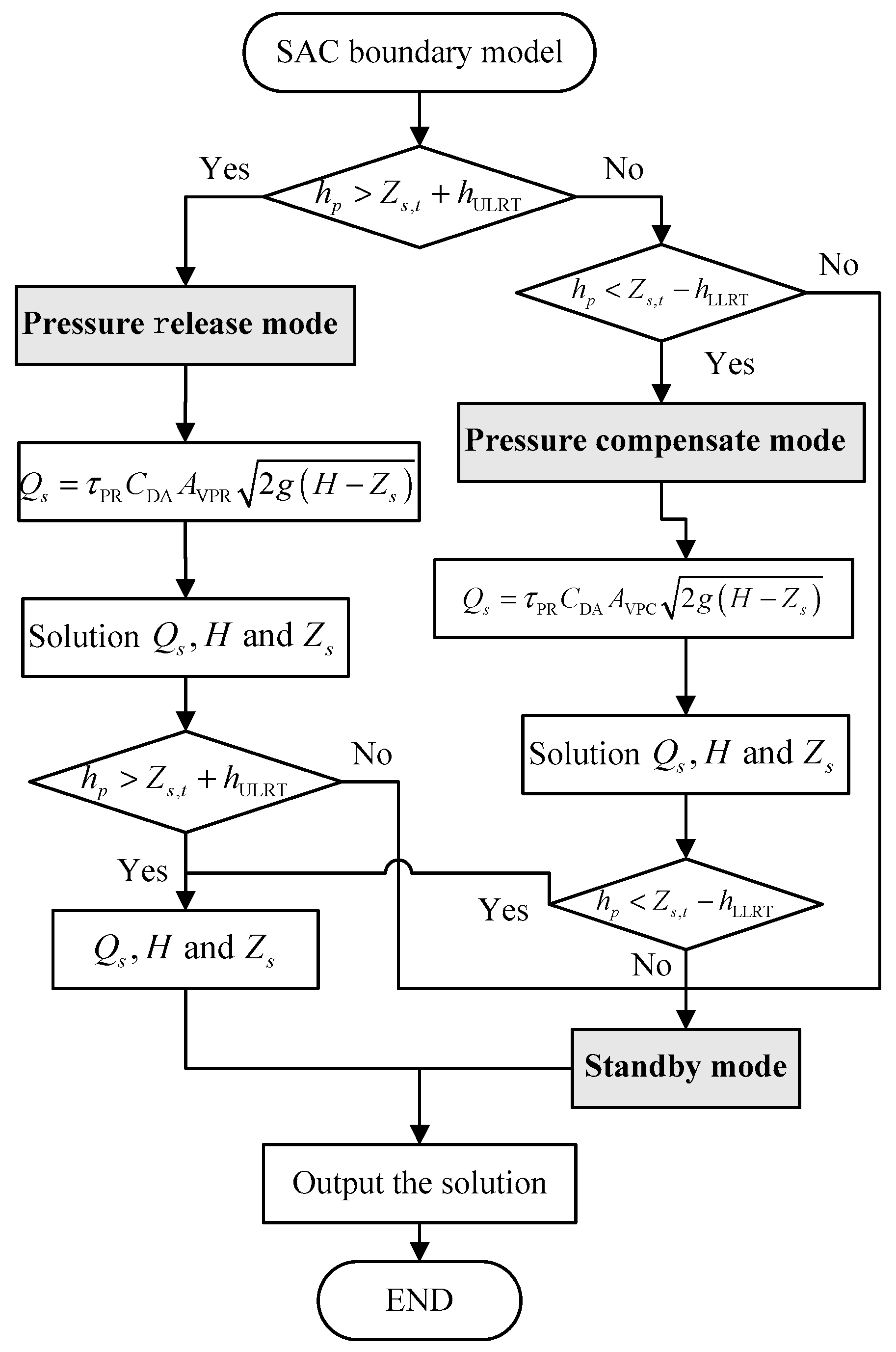
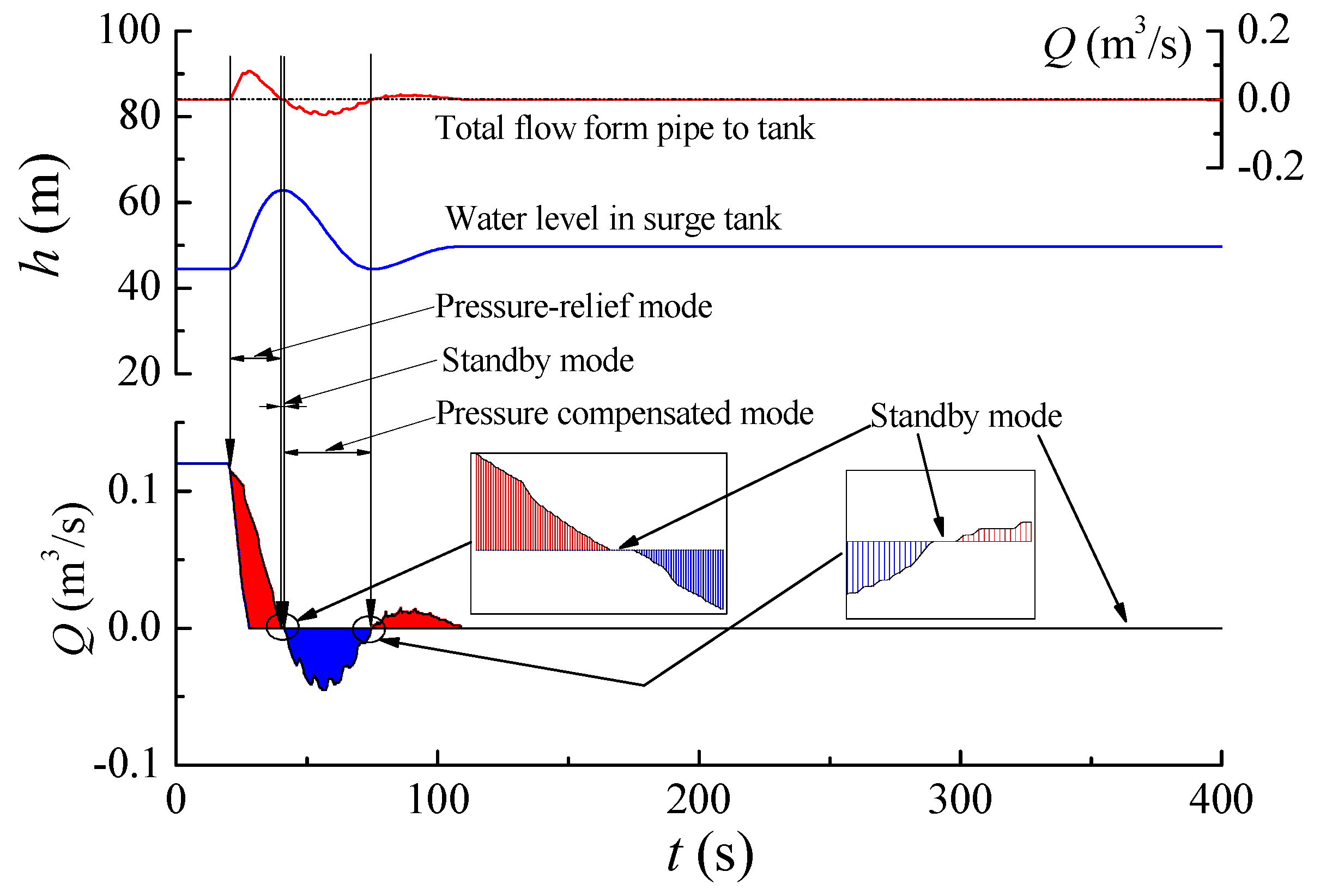
3.2.1. Response Modes of the SAC System

In the surge tank with the SAC system, the complex boundary conditions are divided into various modes, since it can work in various conditions. General contract condition equations are analyzed as follows. Figure 3 shows the three kinds of response modes of SAC, including (a) Standby mode, (b) Pressure release mode, and (c) Pressure compensator mode. In standby status Figure 3a, the PRV and the PCV are both closed and there is no water flow between the surge tank and the main pipe, when the pressure of the main pipe is within SM pressure range of the main pipe. In pressure release mode, seen in Figure 3b, the PRV is activated when the pressure of the pipeline is larger than the upper response threshold (URT), defined as $h_{\mathrm{URT}}$. In other words, the pressure of the pipeline is larger than the pressure of the surge tank and the pressure difference exceeds the upper latency response threshold (ULRT), defined as h_ULRT. At the same time, the PCV keeps closed. In pressure compensate mode (Figure 3c), the PCV is activated when the pressure of the pipeline is lower than the lower response threshold (LRT), defined as $h_{\mathrm{LRT}}$. That means the pressure of the pipeline is lower than the pressure of the surge tank and the pressure difference exceeds the lower latency response threshold (LLRT), defined as $h_{\mathrm{LLRT}}$. At the mode, the PRV keeps closed. The relationships between response threshold and the latency response threshold are $h_{\mathrm{URT}}=Z_{\mathrm{S}}+h_{\mathrm{ULRT}}$ and $h_{\mathrm{LRT}}=Z_{\mathrm{S}}-h_{\mathrm{LLRT}}$, where $Z_s$ is the water level in the surge tank.

In order to simulate the water hammer processes in a RPV closed system, a regular method of characteristics (MOC) boundary model is used [1]. In the regular surge tank, the forward and backward difference equation can be expressed as:

$$\left[\begin{array}{cc}{h}_{i,t+\Delta t}& q_{i,t+\Delta t}\\ h_{j,t+\Delta t}& -q_{j,t+\Delta t}\end{array}\right]\left[\begin{array}{c}1\\ g/aA\end{array}\right]=\left[\begin{array}{c}{h}_{i-1,t}+q_{i-1,t}a/gA-\mathrm{sgn}(q_{i-1,t})f\Delta x{q}_{i-1,t}^2/(2gD{A}^2)\\ h_{j+1,t}-q_{j+1,t}a/gA+\mathrm{sgn}(q_{j-1,t})f\Delta x{q}_{j+1,t}^2/(2gD{A}^2)\end{array}\right]$$

(11)

where, $q$ is the instantaneous discharge at a section.

Obviously, these equations are still valid in the SAC surge tank.

By referring to reference [1] which defined: $B=a/gA$, $R=f\Delta x/(2gD{A}^2)$, $C_{\mathrm{P}}=h_{i-1,t}+B{Q}_{i-1,t}-R{Q}_{i-1,t}\left|Q_{i-1,t}\right|$, $C_{\mathrm{M}}=h_{i+1,t}-B{Q}_{i+1,t}+R{Q}_{i+1,t}\left|Q_{i+1,t}\right|$, then Equation (11) can be simplified as:

$$\left[\begin{array}{c}{h}_{i,t+\Delta t}\\ h_{j,t+\Delta t}\end{array}\right]=\left[\begin{array}{c}{C}_{\mathrm{P}}-B{q}_{i,t+\Delta t}\\ C_{\mathrm{M}}+B{q}_{j,t+\Delta t}\end{array}\right]$$

(12)

To simplify the model, the contract equation can consider both the continuity equation and head equation:

$$\left\{\begin{array}{l}{h}_{i,t+\Delta t}=h_{p,t+\Delta t}\\ h_{j,t+\Delta t}=h_{p,t+\Delta t}\\ \left(Z_{s,t+\Delta t}-Z_{s,t}\right)A_s=\frac{\Delta t}{2}\left(Q_{s,t+\Delta t}+Q_{s,t}\right)\\ Q_{s,t+\Delta t}=q_{i,t+\Delta t}-q_{j,t+\Delta t}\end{array}\right\}$$

(13)

where, $Z_s$ is the water level in the surge tank, and $A_s$ is the cross-sectional area of the surge tank.

Despite this, there are some differences in the discharge between the surge tank and the main pipe. They need to be established separately according to the three response modes of the SAC surge tank. The switching of various modes is shown in Figure 4.

3.2.2. Standby Mode

For the standby mode to happen, the necessary and sufficient conditions are $h_p=\frac{C_{\mathrm{P}}+C_{\mathrm{M}}}{2}$ and $\frac{\Delta t{Q}_{s,t}}{2A_s}+Z_{s,t}-h_{\mathrm{LLRT}}<h_p<\frac{\Delta t{Q}_{s,t}}{2A_s}+Z_{s,t}+h_{\mathrm{ULRT}}$. In this mode, the spring-sleeve control valve and the PCV are both closed and there is no water flow between the surge tank and the main pipe, that is to say, the SAC will not respond to the transient process. Then, the boundary condition can be solved as:

$$\left\{\begin{array}{l}{h}_p=0.5\left(C_{\mathrm{P}}+C_{\mathrm{M}}\right)\\ h_{i,t+\Delta t}=h_p\\ h_{j,t+\Delta t}=h_p\\ q_{i,t+\Delta t}=\left(C_{\mathrm{P}}-h_{i,t+\Delta t}\right)/B\\ q_{j,t+\Delta t}=\left(h_{i,t+\Delta t}-C_{\mathrm{M}}\right)/B\\ Q_{s,t+\Delta t}=q_{i,t+\Delta t}-q_{j,t+\Delta t}\\ Z_{s,t+\Delta t}=Z_{s,t}+0.5\Delta t\left(Q_{s,t+\Delta t}+Q_{s,t}\right)/A_s\end{array}\right\}$$

(14)

3.2.3. Pressure Release Mode

For the pressure release mode, the instantaneous pressure should meet the limit $h_p\in \left(\frac{\Delta t{Q}_{s,t}}{2A_s}+Z_{s,t}+h_{\mathrm{ULRT}},\frac{C_{\mathrm{P}}+C_{\mathrm{M}}}{2}\right)$. The determination condition is $\frac{\Delta t{Q}_{s,t}}{2A_s}+Z_{s,t}+h_{\mathrm{ULRT}}<\frac{C_{\mathrm{P}}+C_{\mathrm{M}}}{2}$, and the SAC will respond to reduce the peak transient pressure. At this time, the main pressure is higher than the active pressure of the SAC, therefore there is flow from the main pipe to the surge tank. The flow discharge can be calculated as follows:

$$Q_{s,t+\Delta t}={\tau }_{\mathrm{PR}}{C}_{\mathrm{DA}}{A}_{\mathrm{VPR}}\sqrt{2g\left(H_{p,t+\Delta t}-Z_{s,t+\Delta t}\right)}$$

(15)

$${\tau }_{\mathrm{PR}}=\min \left(\max \left(0,\frac{\left(h_p-Z_s-h_{\mathrm{ULRT}}\right)}{k_{\mathrm{SFR}}}\right),1\right)$$

(16)

where, $k_{\mathrm{sfr}}$ is the spring coefficient of correlation, $k_{\mathrm{sfr}}=\frac{k{h}_v}{\rho g{A}_v}$, $k_{\mathrm{R}}$ is the spring constant of the pressure release valve, $h_v$ is the height of the spring-sleeve valve, and $A_v$ is the sleeve piston.

$$\begin{array}{r}\frac{C_{\mathrm{P}}+C_{\mathrm{M}}-2h_{i,t+\Delta t}}{B}=\min \left(\max \left(0,\frac{1}{k_{\mathrm{SFR}}}\left(h_p-\left[\frac{\Delta t}{2A_s}\left(\frac{C_{\mathrm{P}}+C_{\mathrm{M}}-2h_{i,t+\Delta t}}{B}+Q_{s,t}\right)+Z_{s,t}\right]-h_{\mathrm{ULRT}}\right)\right),1\right)\\ \times C_{\mathrm{DA}}{A}_{\mathrm{VPR}}\sqrt{2g\left(H_{p,t+\Delta t}-\left[\frac{\Delta t}{2A_s}\left(\frac{C_{\mathrm{P}}+C_{\mathrm{M}}-2h_{i,t+\Delta t}}{B}+Q_{s,t}\right)+Z_{s,t}\right]\right)}\end{array}$$

(17)

Define $x_{\mathrm{p}}=h_{\mathrm{p}}$,

$$\begin{array}{l}\min \left(\max \left(0,\frac{1}{k_{\mathrm{SFR}}}\left[x_{\mathrm{p}}\left(1+\frac{\Delta t}{A_{s}B}\right)-\frac{\Delta t}{2A_{s}B}\left(C_{\mathrm{P}}+C_{\mathrm{M}}+Q_{s,t}B\right)-Z_s-h_{\mathrm{ULRT}}\right]\right),1\right)C_{\mathrm{DA}}\\ \times A_{\mathrm{VPR}}\sqrt{2g\left[x_{\mathrm{p}}\left(1+\frac{\Delta t}{A_{s}B}\right)-\frac{\Delta t}{2A_{s}B}\left(C_{\mathrm{P}}+C_{\mathrm{M}}+Q_{s,t}B\right)-Z_s\right]}+\frac{2x_{\mathrm{p}}}{B}-\frac{C_{\mathrm{P}}+C_{\mathrm{M}}}{B}=0\end{array}$$

(18)

Based on the pressure release mode, limited to $x_{\mathrm{p}}\in \left(\frac{\Delta t{Q}_{s,t}}{2A_s}+Z_{s,t}+h_{\mathrm{ULRT}},\frac{C_{\mathrm{P}}+C_{\mathrm{M}}}{2}\right)$, a monotonically increasing function can be constructed as:

$$\begin{array}{l}f\left(x_{\mathrm{p}}\right)=\min \left(\max \left(0,\frac{1}{k_{\mathrm{SFR}}}\left[x_{\mathrm{p}}\left(1+\frac{\Delta t}{A_{s}B}\right)-\frac{\Delta t}{2A_{s}B}\left(C_{\mathrm{P}}+C_{\mathrm{M}}+Q_{s,t}B\right)-Z_s-h_{\mathrm{ULRT}}\right]\right),1\right)C_{\mathrm{DA}}\\ \times A_{\mathrm{VPR}}\sqrt{2g\left[x_{\mathrm{p}}\left(1+\frac{\Delta t}{A_{s}B}\right)-\frac{\Delta t}{2A_{s}B}\left(C_{\mathrm{P}}+C_{\mathrm{M}}+Q_{s,t}B\right)-Z_s\right]}+\frac{2x_{\mathrm{p}}}{B}-\frac{C_{\mathrm{P}}+C_{\mathrm{M}}}{B}\end{array}$$

(19)

Considering the function is monotonically increasing, there is only one value which can meet the $f\left(x_{\mathrm{p}}\right)=0$. Thus, a procedure of clamp will be adopted to obtain the unique solution. The initial values are defined as:

$$x_{\mathrm{p}1}=\frac{\Delta t{Q}_{s,t}}{2A_s}+Z_{s,t}+h_{\mathrm{ULRT}},x_{\mathrm{p}2}=\frac{C_{\mathrm{P}}+C_{\mathrm{M}}}{2}$$

(20)

Next, if

$$F(x_{\mathrm{p}1})F(\frac{x_{\mathrm{p}1}+x_{\mathrm{p}2}}{2})\le 0,$$

(21)

then,

$$x_{\mathrm{p}2}=(x_{\mathrm{p}1}+x_{\mathrm{p}2})/2,$$

(22)

or else,

$$x_{\mathrm{p}1}=(x_{\mathrm{p}1}+x_{\mathrm{p}2})/2$$

(23)

Repeat this procedure until $x_{\mathrm{p}2}-x_{\mathrm{p}1}\le \epsilon$. Then, $h_p=x_{\mathrm{p}}=(x_{\mathrm{p}1}+x_{\mathrm{p}2})/2$ is considered as the solution.

Figure 5 shows the flow chart of the clamp process. The method has been used in previous research [30] and shows good precision.

After $h_p=(x_{\mathrm{p}1}+x_{\mathrm{p}2})/2$ is solved, all variables can be solved as:

$$\left\{\begin{array}{l}{h}_{i,t+\Delta t}=h_p\\ h_{j,t+\Delta t}=h_p\\ q_{i,t+\Delta t}=\left(C_{\mathrm{P}}-h_{i,t+\Delta t}\right)/B\\ q_{j,t+\Delta t}=\left(h_{i,t+\Delta t}-C_{\mathrm{M}}\right)/B\\ Q_{s,t+\Delta t}=q_{i,t+\Delta t}-q_{j,t+\Delta t}\\ Z_{s,t+\Delta t}=Z_{s,t}+0.5\Delta t\left(Q_{s,t+\Delta t}+Q_{s,t}\right)/A_s\end{array}\right\}$$

(24)

3.2.4. Pressure Compensate Mode

When $\frac{C_{\mathrm{P}}+C_{\mathrm{M}}}{2}<h_p<\frac{\Delta t{Q}_{s,t}}{2A_s}+Z_{s,t}-h_{\mathrm{LLRT}}$, the surge tank will be activated as the pressure compensate mode. When the determination condition is $\frac{C_{\mathrm{P}}+C_{\mathrm{M}}}{2}<\frac{\Delta t{Q}_{s,t}}{2A_s}+Z_{s,t}-h_{\mathrm{LLRT}}$, the SAC will respond to increase the trough transient pressure. At this time, there is flow from the surge tank to the main pipe.

$$Q_{s,t+\Delta t}=-{\tau }_{\mathrm{PC}}{C}_{DA}{A}_{\mathrm{VPC}}\sqrt{-2g\left(H_{p,t+\Delta t}-Z_{s,t+\Delta t}\right)}$$

(25)

$${\tau }_{\mathrm{PC}}=\min \left(\max \left(0,\frac{\left(Z_s-h_{\mathrm{LLRT}}-h_p\right)}{k_{\mathrm{SFC}}}\right),1\right)$$

(26)

where, $\tau$ is the cylinder’s opening ratio, $C_{DA}$ is the discharge coefficient of the valve, and $A$ is the cross area. Analogously,

$$\begin{array}{r}\frac{C_{\mathrm{P}}+C_{\mathrm{M}}-2h_{i,t+\Delta t}}{B}=-\min \left(\max \left(0,\frac{1}{k_{\mathrm{SFC}}}\left(\left[\frac{\Delta t}{2A_s}\left(\frac{C_{\mathrm{P}}+C_{\mathrm{M}}-2h_{i,t+\Delta t}}{B}+Q_{s,t}\right)+Z_{s,t}\right]-h_p-h_{\mathrm{LLRT}}\right)\right),1\right)\\ \times C_{\mathrm{DA}}{A}_{\mathrm{VPC}}\sqrt{-2g\left(H_{p,t+\Delta t}-\left[\frac{\Delta t}{2A_s}\left(\frac{C_{\mathrm{P}}+C_{\mathrm{M}}-2h_{i,t+\Delta t}}{B}+Q_{s,t}\right)+Z_{s,t}\right]\right)}\end{array}$$

(27)

According to the mode condition, limited to $x\in \left(\frac{C_{\mathrm{P}}+C_{\mathrm{M}}}{2},\frac{\Delta t{Q}_{s,t}}{2A_s}+Z_{s,t}-h_{\mathrm{LLRT}}\right)$, a monotonic decreasing function can be constructed as:

$$\begin{array}{r}f\left(x_p\right)=-\min \left(\max \left(0,\frac{1}{k_{\mathrm{SFC}}}\left(\left[\frac{\Delta t}{2A_s}\left(\frac{C_{\mathrm{P}}+C_{\mathrm{M}}-2h_{i,t+\Delta t}}{B}+Q_{s,t}\right)+Z_{s,t}\right]-x_p-h_{\mathrm{LLRT}}\right)\right),1\right)\\ \times C_{\mathrm{DA}}{A}_{\mathrm{VPC}}\sqrt{-2g\left(H_{p,t+\Delta t}-\left[\frac{\Delta t}{2A_s}\left(\frac{C_{\mathrm{P}}+C_{\mathrm{M}}-2h_{i,t+\Delta t}}{B}+Q_{s,t}\right)+Z_{s,t}\right]\right)}-\frac{2x_p}{B}+\frac{C_{\mathrm{P}}+C_{\mathrm{M}}}{B}\end{array}$$

(28)

Analogously to Section 3.2.3, the $h_p=x_p$ can be solved, and then all variables can be solved as:

$$\left\{\begin{array}{l}{h}_{i,t+\Delta t}=h_p\\ h_{j,t+\Delta t}=h_p\\ q_{i,t+\Delta t}=\left(C_{\mathrm{P}}-h_{i,t+\Delta t}\right)/B\\ q_{j,t+\Delta t}=\left(h_{i,t+\Delta t}-C_{\mathrm{M}}\right)/B\\ Q_{s,t+\Delta t}=q_{i,t+\Delta t}-q_{j,t+\Delta t}\\ Z_{s,t+\Delta t}=Z_{s,t}+0.5\Delta t\left(Q_{s,t+\Delta t}+Q_{s,t}\right)/A_s\end{array}\right\}$$

(29)

3.3. Boundary Conditions

3.3.1. Inlet Reservoir Boundary Condition

For an upstream reservoir system, the water level can be considered as the constant. The common boundary contract can be written as [29]:

$$\left\{h_i^{t+\Delta t}=C,\frac{\partial h_i}{\partial t}=0\right\}$$

(30)

Use a forward difference,

$$\frac{\partial h_i^{t+\Delta t}}{\partial t}=-v_i^{t+\Delta t}\frac{h_{i+1}^{t+\Delta t}-h_i^{t+\Delta t}}{\Delta x}-\frac{a^2}{g}\frac{v_{i+1}^{t+\Delta t}-v_i^{t+\Delta t}}{\Delta x}+v_i^{t+\Delta t}\sin \theta$$

(31)

Then, the solution of the inlet node can be written as:

$$\left[\begin{array}{c}{h}_i^{t+\Delta t}\\ v_i^{t+\Delta t}\end{array}\right]=\left[\begin{array}{c}C\\ -a^2{v}_{i+1}^{t+\Delta t}/\left[(h_{i+1}^{t+\Delta t}-h_i^{t+\Delta t}-\Delta x\sin \theta )g-a^2\right]\end{array}\right]$$

(32)

3.3.2. Valve Boundary Control Equation

In a RLV system, the opening and closing of the valve can generate a water hammer. The boundary condition of the valve usually depends on the discharge characteristics. If we consider the end as the datum in the MCMT scheme, the contract equation of the valve can be written as [29]:

$$\left[\begin{array}{c}{h}_{ns}^{t+\Delta t}\\ v_{ns}^{t+\Delta t}\end{array}\right]=\left[\begin{array}{c}{h}_{ns}\\ h_{ns}{C}_d\sqrt{2g{h}_{ns}}\end{array}\right]|\begin{array}{}\\ h_{ns}=2h_{ns-1}^{t+\Delta t}-h_{ns-2}^{t+\Delta t}\end{array}$$

(33)

3.4. Initial State Conditions

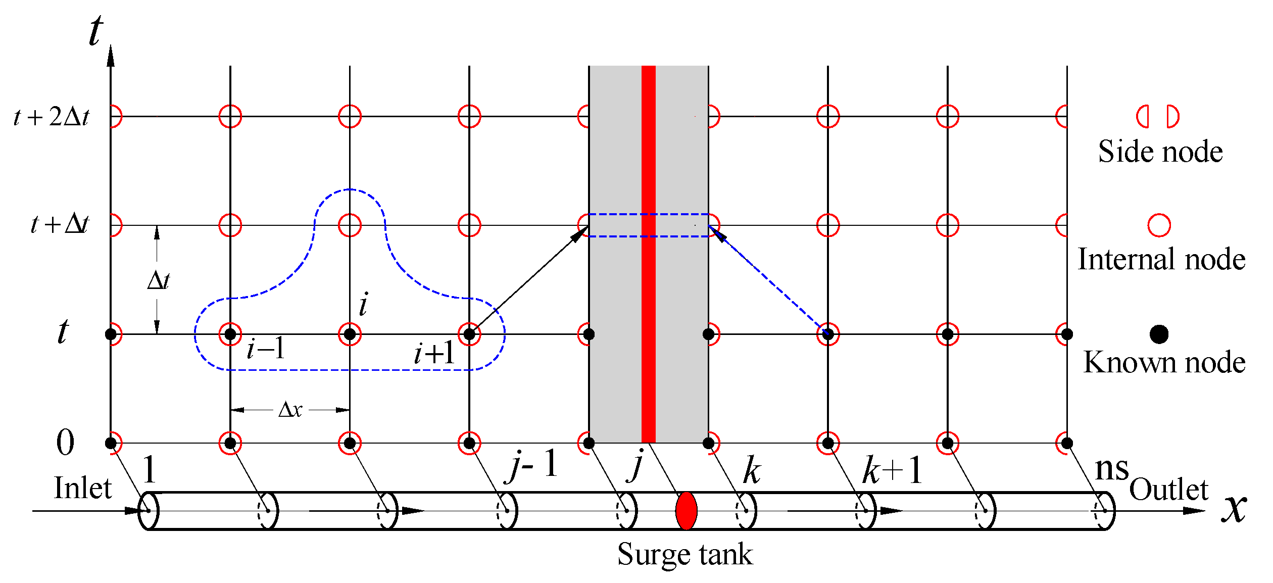
The initial condition, with all values at time 0, can usually be determined on the initial steady-flow state. According to the steady condition, the boundary condition can be numerically expressed as:

$$\left[\begin{array}{c}{v}_i=v_0{A}_0/A_{i}i=1,2\cdots n\\ {h_{i+1}=h_i-h_w^{\stackrel{⌢}{i,i+1}}|}_{h_1=h_0}i=1,2\cdots n\end{array}\right]|\begin{array}{}\\ \\ t=0\end{array}$$

(34)

3.5. Discrete Grid

In order to establish the numerical calculation, the time and space steps are set according to the following regulation:

$$n=\mathrm{int}\left(\frac{\Delta x}{a\Delta t}+0.5\right)+1$$

(35)

The meshing is adjusted to the method of characteristics (MOC) in order to deal with the boundary condition nodes.

4. Simulation and Result Analysis

4.1. The Response Principle of the Surge Tank without SAC

A common RLV system, as shown in Figure 6, is separately considered with a regular surge tank and a SAC surge tank. The system parameters are shown in

Table 1. Parameters of the pipe and surge tank.

Parameters	Value
Water level of the upstream reservoir ($H_0$)	52.40 m
Length of the pipe ($L_{\mathrm{p}}$)	2820 m
Rated discharge of the pipeline ($Q$)	0.12 m3/s
Wave speed of water hammer ($a$)	1,000 m/s
Time of closing valve ($T_{\mathrm{c}}$)	8.0 s
Diameter of the main pipe ($D$)	0.40 m
Section of the surge tank ($A_{\mathrm{S}}$)	0.05 m2

.

Figure 7 shows the pressure wave upstream of the valve. As shown in Figure 7, the surge tank can significantly mitigate the fluctuation of the transient pressure. Moreover, Figure 8 shows the basic response mechanism of the surge tank. As shown in Figure 8, when the pressure increases in the pipe, the surge tank always absorbs water from the pipe to prevent the increase of the transient pressure (PRM). Conversely, when the pressure decreases in the pipe, the surge tank will release water to the main pipe to prevent the decrease of the transient pressure (PCM). Obviously, the surge tank reduces the peak pressure from 116.56 m to 72.43 m and increases the negative pressure from −2.44 m to 37.36 m. As shown in Figure 7, the water level fluctuates between 37.36 m and 72.43 m. Therefore, the top elevation of the surge tank must be more than 34.93 m, and the bottom elevation of the surge tank must be less than 37.36 m. The effective height of the surge tank must be greater than 72.43 m to ensure the exchange of water during pressure regulation.

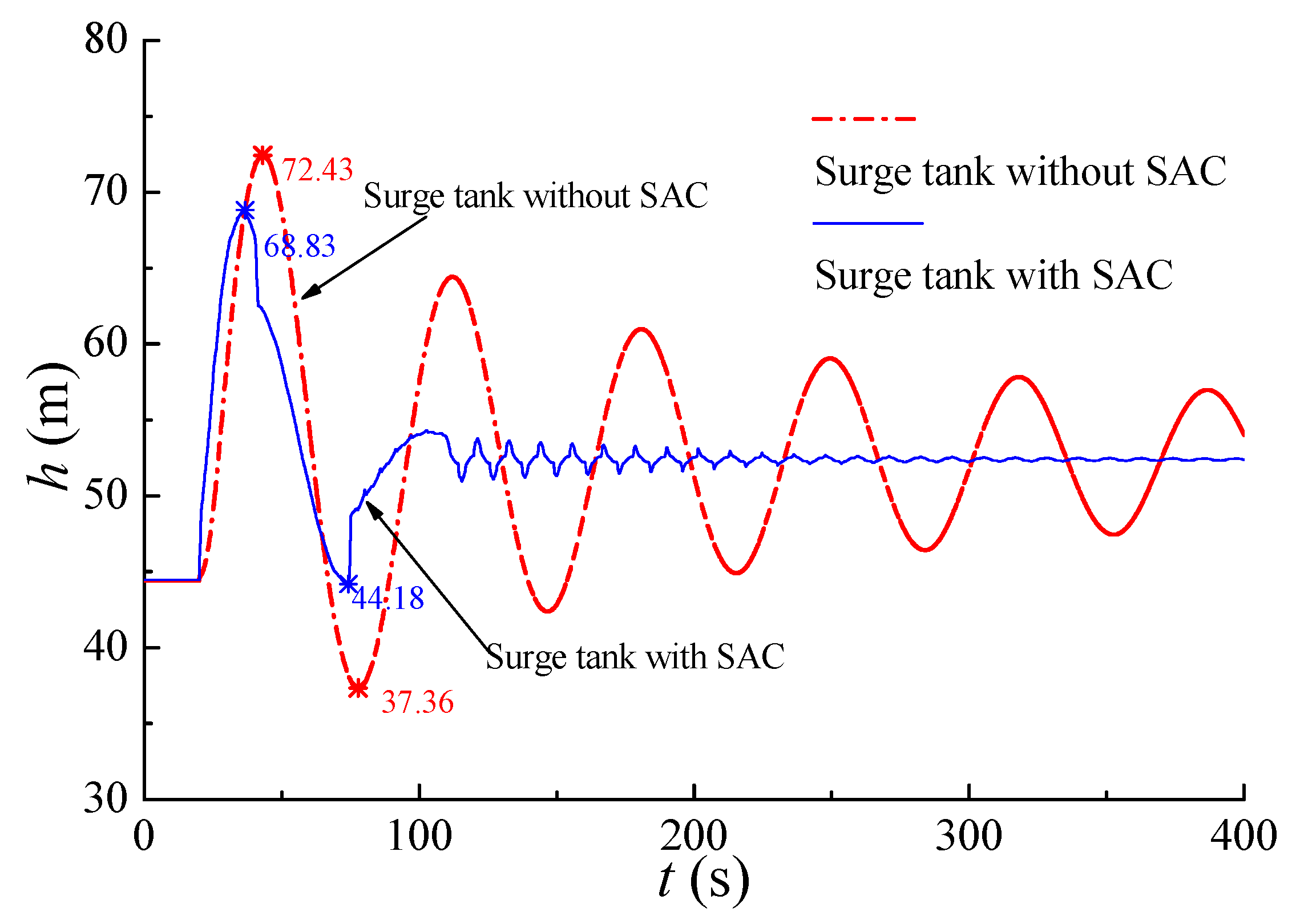
4.2. Improved Surge Tank by a SAC

As seen in Figure 8, the surge tank always works no matter whether the transient pressure exceeds the tolerable range of the pipe system. Therefore, the water level in the surge tank rises and falls greatly with the fluctuation of the pipe pressure during the transient process. Consequently, a large-scale surge tank is usually necessary to cover the amplitude of fluctuation and store enough water. In fact, the surge tank does not need to respond if the transient pressure does not exceed the allowable range of the pipe. It may work more efficiently if the surge tank is activated only when the pressure exceeds the preset pressure threshold value.

In this case, a smaller-scale surge tank may be enough to meet the same effect. In order to improve the properties of the surge tank, the mechanical auxiliary control proposed in Section 2.2 is installed and investigated in the same case. The parameters of the SAC system are shown in

Table 2. Parameters of the SAC.

Parameters	Value
Latency response threshold of release valve ($h_{\mathrm{ULRT}}$)	4.0 m
Spring orifice coefficient ($k_{\mathrm{SFR}}$)	28.6
Discharge coefficient of release valve ($C_{d\mathrm{r}}$)	0.65
The nominal area of release valve orifice ($A_{\mathrm{VPR}}$)	0.037 m2
Latency response threshold of compensate valve ($h_{\mathrm{LLRT}}$)	0.20 m
Spring orifice coefficient ($k_{\mathrm{SFC}}$)	0.5
Discharge coefficient of compensate valve ($C_{\mathrm{dc}}$)	0.80
The nominal area of compensate valve orifice ($A_{\mathrm{VPC}}$)	0.03 m2

.

Figure 9 compares the transient pressure with or without the SAC system. With the SAC system, the peak pressure of transient flow decreases from 72.43 m to 68.83 m, the trough pressure of transient flow increases from 37.36 m to 44.18 m, and the fluctuation amplitude decreases by 10.42 m. As shown in Figure 9, the device can reduce the peak pressure and increase the trough pressure, thus reducing the amplitude of pressure fluctuation.

Figure 10 shows the discharge process of the intelligent surge tank during the water hammer process. In the pressure release mode, when the pressure rises above the upper critical value, the pressure-releasing orifice is activated, and the surge tank absorbs water to reduce the peak pressure of the pipe system. Subsequently, when the pressure recovers below the upper critical pressure, the pressure-releasing orifice closes. In the pressure compensate mode, when the pressure drops below the lower critical value, the pressure compensation orifice is activated and the surge tank releases water to increase the trough pressure of the pipe system. Subsequently, when the pressure recovers above the lower critical pressure, the pressure compensation orifice closes. After several reciprocating fluctuations, the pressure will be controlled between the upper and lower critical values. As shown in Figure 10, with the SAC, the water exchange capacity of pipelines and the surge tank is smaller, so the volume required for the surge tank is reduced.

If the pressure is between the upper and lower response threshold values, both the PRV and the PCV are closed. At this time, the surge tank keeps its standby state. When activated, the frequency of transient flow depends on the surge tank and pipeline, while the fluctuation frequency only depends on the pipeline when the SAC system is not activated. The maximum peak pressure occurs in the first response of the pressure-releasing orifice, and the minimum trough pressure occurs in the first response of the pressure compensation orifice.

Figure 11 shows the changing process of upper and lower response threshold values to active various modes with the water level of the surge tank, the transient pressure process at the valve, as well as the opening and flow process of the PRV and the PCV. The results show that the water level changes due to the inflow and outflow of the surge tank, and the upper and lower response threshold values also change correspondingly, which is also related to the initial water level of the surge tank. The upper response threshold value is the instantaneous water level of the surge tank plus the response threshold, and the lower response threshold value is the instantaneous water level of the surge tank minus the response threshold. When the pipeline pressure exceeds the envelope curve of the response threshold value, the surge tank begins to respond. Conversely, when the pressure enters between the upper and lower response threshold values, the throttles of the surge tank will close, and the SAC returns to its standby state.

As shown in Figure 8, for the regular surge tank, it is always active during the operation conditions, consequently, the surge tank needs to have enough height to meet the water level fluctuation. However, the proposed surge tank is only active with the most effective work conditions. As seen in Figure 11, with SAC equipment, the improved surge tank can automatically respond according to the instantaneous transient intensity. In the same case, the water level fluctuation of the intelligent mechanical surge tank is less than that of the regular surge tank without SAC equipment, so the requested size becomes smaller for the intelligent surge tank.

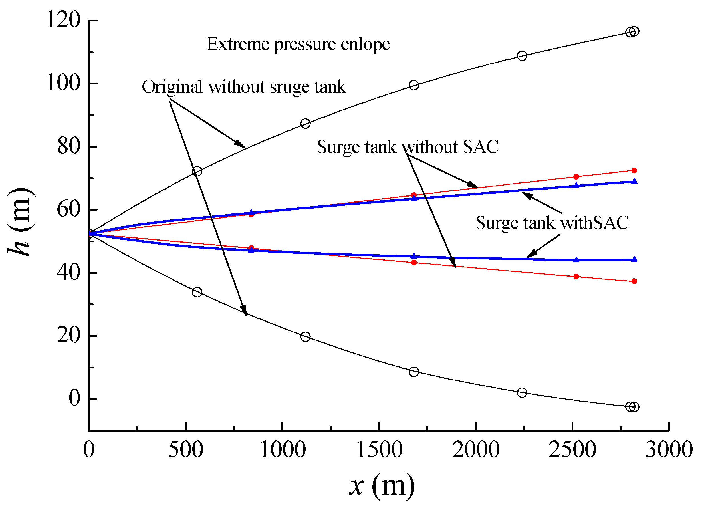
4.3. Results and Verification

Figure 12 shows the pressure fluctuation process of pipeline control points in three cases in the original pipeline respectively, with a regular surge tank and a SAC surge tank. The original maximal pressure of the pipeline is 116.56 m, in which the maximal pressure decreased to 72.43 m with a regular surge tank, while the maximal pressure reduced to 68.83 m with a SAC surge tank. Moreover, Figure 13 shows the extreme pressure distribution along the pipeline for various water hammer protection conditions. Compared with the regular surge tank without the SAC system, the surge tank with the SAC system can improve the water hammer control properties of the surge tank, not only the pressure fluctuation of the key section, but also the whole distribution of the extreme pressure.

For the water level oscillation, it is the basis for selecting the size of the surge tank in the design stage. Figure 14 shows the comparison of water level oscillations in various surge tanks. Obviously, with an intelligent surge tank with the SAC system, the water oscillation can be better controlled between the pipe elevation and the ground elevation. The required height of the surge tank decreases from 35.07 m to 18.34 m. In this way, the surge tank can be conveniently set.

The results show that the SAC system can greatly improve the regular surge tank in both the transient pressure control of the pipeline and water level oscillation control of the surge tank. With the SAC system, not only can the transient pressure of the pipeline be better controlled, but also the water level height of the surge tank can be greatly reduced, which can reduce the vertical size of the surge tank.

5. Analysis and Discussion

As is known in steady flow, the water level of the conventional surge tank is always consistent with the hydraulic pressure head of the protected pipeline. Even if the throttle is set, the surge tank always responds in real time regardless of whether the transient pressure fluctuation is within the allowable operating range of the pipe. Therefore, a larger height of the surge tank is necessary, since the water level fluctuations are severe in the surge tank. If the response of the surge tank is optimally controlled, that is to say the surge tank responds only when the transient pressure exceeds a specific range, in this way we can improve the efficiency of the surge tank and reduce the size required. In order to improve the performance of the surge tank, an intelligent self-adaptive auxiliary control system was proposed. The self-adaptive auxiliary control system can divide the surge tank with three response states by setting the inlet and outlet orifices. The improved surge tank can only respond when the upper and lower response threshold values are exceeded. Compared with conventional surge tanks, intelligent surge tanks take smaller water exchange capacity and the water level fluctuations are smaller in amplitude. Therefore, the efficiency of the surge tank is higher in this case. Accordingly, a smaller scale is required to perform the same functions as a conventional surge tank. An improved surge tank can reduce peak pressure, increase trough pressure, and achieve better pressure control in pipelines by reducing the fluctuation range. It also makes large fluctuations decay faster to the threshold range. Therefore, the SAC system can not only control the maximum oscillation amplitude, but also reduce the risk of reciprocating significant oscillation. On the downside, additional mechanical equipment may complicate the surge tank in design and construction, as well as maintenance.

6. Conclusions

In this paper, the SAC system was proposed to improve the water control performance of the regular surge tank. Then, the numerical model and matching boundary conditions were established to simulate and analyze the water hammer control of the surge tank with SAC. The results show that the SAC system can improve the operation performance and make the surge tank work more efficiently by setting various response modes, which are controlled by the spring-sleeve pressure release valve (PRV) and the spring-sleeve pressure compensator valve (PCV). The proposed system can reduce the peak pressure and increase the trough pressure in the pipe system, as well as reduce the amplitude of the water level in the surge tank. The improved surge tank can attenuate the large amplitude oscillation faster, and then control the transient pressure waves within the threshold envelope. The results show that the fluctuation of the water level in the surge tank is greatly decreased with the SAC system, thus the required size is smaller than that the regular surge tank. Therefore, the SAC system can further optimize the surge tank both in transient pressure control of the pipeline and the water level oscillation of the surge tank, as well as reduce the required vertical scale of the surge tank.

References

1. Wylie, E.B.; Streeter, V.L. Fluid Transients; McGraw-Hill International Book Co.: New York, NY, USA, 1978. [Google Scholar]
2. Wan, W.; Huang, W. Investigation on complete characteristics and hydraulic transient of centrifugal pump. J. Mech. Sci. Technol. 2011, 25, 2583–2590. [Google Scholar] [CrossRef]
3. Hur, J.; Kim, S.; Kim, H. Water hammer analysis that uses the impulse response method for a reservoir-pump pipeline system. J. Mech. Sci. Technol. 2017, 31, 4833–4840. [Google Scholar] [CrossRef]
4. Kim, S.G.; Lee, K.B.; Kim, K.Y. Water hammer in the pump-rising pipeline system with an air chamber. J. Hydrodyn. 2014, 26, 960–964. [Google Scholar] [CrossRef]
5. Rohani, M.; Afshar, M.H. Simulation of transient flow caused by pump failure: Point-Implicit Method of Characteristics. Ann. Nucl. Energy 2010, 37, 1742–1750. [Google Scholar] [CrossRef]
6. Guo, W.C.; Yang, J.D.; Teng, Y. Surge wave characteristics for hydropower station with upstream series double surge tanks in load rejection transient. Renew. Energy 2017, 108, 488–501. [Google Scholar] [CrossRef]
7. Liu, J.; Zhang, J.; Chen, S.; Yu, X. Investigation on Maximum Upsurge and Air Pressure of Air Cushion Surge Chamber in Hydropower Stations. J. Press. Vessel Technol. 2017, 139, 031603. [Google Scholar] [CrossRef]
8. Riasi, A.; Tazraei, P. Numerical analysis of the hydraulic transient response in the presence of surge tanks and relief valves. Renew. Energy 2017, 107, 138–146. [Google Scholar] [CrossRef] [Green Version]
9. Duan, H.F.; Tung, Y.K.; Ghidaoui, M.S. Probabilistic Analysis of Transient Design for Water Supply Systems. J. Water Resour. Plan. Manag. 2010, 136, 678–687. [Google Scholar] [CrossRef]
10. Kim, S.H. Design of surge tank for water supply systems using the impulse response method with the GA algorithm. J. Mech. Sci. Technol. 2010, 24, 629–636. [Google Scholar] [CrossRef]
11. Zhang, B.R.; Wan, W.Y.; Shi, M.S. Experimental and Numerical Simulation of Water Hammer in Gravitational Pipe Flow with Continuous Air Entrainment. Water 2018, 10, 928. [Google Scholar] [CrossRef]
12. Collins, R.P.; Boxall, J.B.; Karney, B.W.; Brunone, B.; Meniconi, S. How severe can transients be after a sudden depressurization? J. Am. Water Work Assoc. 2012, 104, 67–68. [Google Scholar] [CrossRef]
13. Behbahani-Nejad, M.; Bagheri, A. The accuracy and efficiency of a MATLAB-Simulink library for transient flow simulation of gas pipelines and networks. J. Pet. Sci. Eng. 2010, 70, 256–265. [Google Scholar] [CrossRef]
14. Esmaeilzadeh, F.; Mowla, D.; Asemani, M. Mathematical modeling and simulation of pigging operation in gas and liquid pipelines. J. Pet. Sci. Eng. 2009, 69, 100–106. [Google Scholar] [CrossRef]
15. Vakil, A.; Firoozabadi, B. Investigation of Valve-Closing Law on the Maximum Head Rise of a Hydropower Plant. Sci. Iran. Trans. B Mech. Eng. 2009, 16, 222–228. [Google Scholar]
16. Bazargan-Lari, M.R.; Kerachian, R.; Afshar, H.; Bashi-Azghadi, S.N. Developing an optimal valve closing rule curve for real-time pressure control in pipes. J. Mech. Sci. Technol. 2013, 27, 215–225. [Google Scholar] [CrossRef]
17. Zhou, J.Z.; Xu, Y.H.; Zheng, Y.; Zhang, Y.C. Optimization of Guide Vane Closing Schemes of Pumped Storage Hydro Unit Using an Enhanced Multi-Objective Gravitational Search Algorithm. Energies 2017, 10, 911. [Google Scholar] [CrossRef]
18. Wan, W.; Li, F. Sensitivity Analysis of Operational Time Differences for a Pump–Valve System on a Water Hammer Response. J. Press. Vessel Technol. 2016, 138, 011303. [Google Scholar] [CrossRef]
19. Kim, H.; Kim, S.; Kim, Y.; Kim, J. Optimization of Operation Parameters for Direct Spring Loaded Pressure Relief Valve in a Pipeline System. J. Press. Vessel Technol. Trans. Asme 2018, 140, 051603. [Google Scholar] [CrossRef]
20. Triki, A.; Chaker, M.A. Compound technique-based inline design strategy for water-hammer control in steel pressurized-piping systems. Int. J. Press. Vessel. Pip. 2019, 169, 188–203. [Google Scholar] [CrossRef]
21. Triki, A. Dual-technique-based inline design strategy for water-hammer control in pressurized pipe flow. Acta Mech. 2018, 229, 2019–2039. [Google Scholar] [CrossRef]
22. Triki, A. Water-hammer control in pressurized-pipe flow using an in-line polymeric short-section. Acta Mech. 2016, 227, 777–793. [Google Scholar] [CrossRef]
23. Wylie, E.B.; Streeter, V.L.; Suo, L. Fluid Transients in Systems; Prentice Hall: Englewood Cliffs, NJ, USA, 1993. [Google Scholar]
24. Pezzinga, G. Evaluation of unsteady flow resistances by quasi-2D or 1D models. J. Hydraul. Eng. 2000, 126, 778–785. [Google Scholar] [CrossRef]
25. Pezzinga, G. Discussion of ‘Developments in unsteady pipe flow friction modelling’. J. Hydraul. Res. 2002, 40, 650–653. [Google Scholar]
26. Bergant, A.; Simpson, A.R.; Vitkovsky, J. Developments in unsteady pipe flow friction modelling. J. Hydraul. Res. 2001, 39, 249–257. [Google Scholar] [CrossRef] [Green Version]
27. Vardy, A.E.; Brown, J.M.B. On Turbulent, Unsteady, Smooth-Pipe Flow. In Proceedings of the International Conference on Pressure Surges and Fluid Transients, Harrogate, UK, 16–18 April 1994; BHR Group: Harrogate, UK, 1996; pp. 289–311. [Google Scholar]
28. Brunone, B.; Golia, U.M.; Greco, M. Effects of 2-dimensionality on pipe transients modeling. J. Hydraul. Eng. 1995, 121, 906–912. [Google Scholar] [CrossRef]
29. Wan, W.; Huang, W. Water hammer simulation of a series pipe system using the MacCormack time marching scheme. Acta Mech. 2018, 229, 3143–3160. [Google Scholar] [CrossRef]
30. Wan, W.; Huang, W.; Li, C. Sensitivity Analysis for the Resistance on the Performance of a Pressure Vessel for Water Hammer Protection. J. Press. Vessel Technol. Trans. Asme 2014, 136, 011303. [Google Scholar] [CrossRef]
Figure 1. Comparison of different surge tank arrangements.
Energies 12 02527 g001
Figure 2. Time-marching mesh for the pipe flow with surge tank.
Energies 12 02527 g002
Figure 3. The response modes of the self-adaptive auxiliary control (SAC) system. (a) Standby mode, (b) Pressure release mode, (c) Pressure compensate mode.
Energies 12 02527 g003
Figure 4. Flowchart of the simulation of the intelligent surge tank (IST) with SAC.
Energies 12 02527 g004
Figure 5. The flowchart of the iterative process.
Energies 12 02527 g005
Figure 6. Intelligent surge tank in reservoir pipeline valve system.
Energies 12 02527 g006
Figure 7. Transient pressure induced by a valve close.
Energies 12 02527 g007
Figure 8. Response principle of the regular surge tank.
Energies 12 02527 g008
Figure 9. Transient pressure comparison of the surge tanks with or without SAC.
Energies 12 02527 g009
Figure 10. Flow process in surge tank with the pressure.
Energies 12 02527 g010
Figure 11. Water hammer control of intelligent surge tank with SAC.
Energies 12 02527 g011
Figure 12. Comparison of the pressure fluctuation process of pipeline control points.
Energies 12 02527 g012
Figure 13. Comparison of the extreme pressure along the pipeline.
Energies 12 02527 g013
Figure 14. Comparison of the water level fluctuation of the surge tanks.
Energies 12 02527 g014