Abstract
Rising levels of variable renewable energy (VRE) in Australia’s National Electricity Market have been driven by a 20% renewable energy target by 2020. This certificated renewable portfolio standard has successfully driven new investment, allocated risk amongst buy- and sell-side market participants and met overall policy objectives. But a policy vacuum for achieving long-term CO2 emission targets post-2020 has led to sub-national and, potentially, national governments initiating contract-for-differences (CfDs) to drive further investment activity in new plant—with virtually no coordination between the jurisdictions. In a gross pool energy-only market setting, replacing on-market transactions between retailers and generators with off-market transactions between governments and generators may have unintended side-effects vis-à-vis market stability. In this article, an energy-only gross pool is modeled with rising levels of off-market government-initiated CfDs, with a specific focus on spot and forward contract market outcomes. Model results show that as VRE plant enters, coal plant exit, and on-market firm hedge contracts historically supplied by coal plant are progressively replaced by off-market CfDs. In the event, while a tractable equilibrium can be maintained in the spot market, shortages of “primary issuance” hedge contracts emerge in the forward market. Any shortage of hedge contract capacity is likely to raise forward contract price premiums above efficient levels, force price-elastic customers into accepting unwanted spot market exposures and may unintentionally foreclose non-integrated (2nd tier) energy retailers, all of which harms consumer welfare. A wide-ranging program of government CfDs may therefore not be compatible with an energy-only market design.
1. Introduction
1.1. Background to Australia’s National Electricity Market
Australia’s National Electricity Market (NEM) is an energy-only gross pool in which all generators bid into a central platform and are dispatched under a uniform first-price auction clearing mechanism. Being a mandatory gross pool, all generators must sell their output in the spot market, and energy retailers must buy all load from the spot market.
The volatility that accompanies organized energy-only spot markets, particularly those with a high VoLL (NEM value of lost load at AUD $14,500/MWh is amongst the highest in the world) creates the conditions necessary for active trade in forward contracts. While there is an almost endless array of derivative instruments, the three most commonly traded contracts are swaps, $300 caps and increasingly, run-of-plant power purchase agreements (PPAs). Swaps and caps are traded both on-exchange and over-the-counter, generally over a 1–3 year tenor at quarterly resolution, with market liquidity running at ~300% of physical trade and considerable variation in liquidity by season and region. PPAs on the other hand tend to be long-dated (10–15 year), structured as run-of-plant instruments and designed specifically to underwrite the entry of variable renewable energy (VRE), that is, wind or utility-scale solar PV, with the market characterized by a small number of buyers and a large number of (potential) sellers/developers.
Australia’s 20% renewable energy target (RET) is a renewable portfolio standard that requires energy retailers achieve a 20% renewable market share by 2020. The broad-based market scheme is mobilized through the trade of renewable energy certificates, and has been highly successful in facilitating VRE plant entry. The 20% RET is expected to be comfortably met by 2020.
Once the 20% RET has been met, the NEM faces a virtual policy vacuum in terms of future CO2 emissions reductions. The most recent attempt (in 2018) at designing a bipartisan approach to reduce power sector CO2 emissions in a manner compatible with Australia’s international obligations and the NEM’s energy-only market design involved a scheme known as the National Energy Guarantee. This market-based scheme was comprised of a reliability obligation (plant capacity) and an emissions obligation (CO2 emissions), with energy retailers being the liable parties. But landing a united energy and climate change policy architecture to guide the NEM’s ongoing transition has proven to be a complex political task [1,2]. Indeed, the politics of a two-decades-long climate change policy war has underpinned the downfall of at least three sitting Australian Prime Ministers since 2010, including Prime Minister Malcolm Turnbull (by his own party) whilst pursuing the National Energy Guarantee.
Policy discontinuity has led to cyclical swings in VRE plant investment commitments. The Commonwealth Government’s decision to review the 20% RET in early-2014 produced sufficient policy uncertainty to induce a transient cessation in buy-side PPA activity—such instruments typically being an essential ingredient to VRE project commitment in an energy-only market [2].
One response to the Commonwealth Government’s climate change policy discontinuity has been the emergence of government-initiated contracts-for-differences (CfDs) undertaken unilaterally by sub-national governments—first by the Australian Capital Territory (wind, 2015), then Queensland (solar PV, 2016), South Australia (semi-CfD for battery storage, 2017) and Victoria (wind and solar PV, 2018). These targeted, centrally planned CfD auctions have been successful at meeting their policy objectives.
The Commonwealth election in mid-2019 gave rise to two distinct policy choices at the national level. The incumbent conservative Liberal government sought to underwrite new “dispatchable” (i.e., coal, gas, pumped-hydro) generation in order to reduce energy prices by way of government-initiated CfDs. The democratic Labor opposition on the other hand sought to revive the Liberal government’s National Energy Guarantee in order to reduce CO2 emissions and provide the policy stability sought by market participants to guide ongoing investment in on-market transactions. However, if bipartisan support for the National Energy Guarantee could be achieved, Labor would default to a wide-ranging program of centrally planned CfDs to ensure ongoing VRE investment continuity to meet a 50% renewable target by 2030.
Government-initiated and taxpayer-funded CfDs are an interesting development [3,4]. CfDs can play a legitimate role in dealing with energy market failures relating to missing policy, missing markets and incomplete markets. As a policy mechanism, they represent a means by which to deliver generation plant capacity that, for whatever reason, the market is failing to deliver. Government-initiated CfDs have the effect of diversifying buy-side forward market liquidity and in doing so bring about certain short run benefits. Holding all else constant, apart from reducing CO2 emissions, VRE CfDs facilitate state/regional economic development and by adding new renewable supply can reduce spot prices, at least on a transient basis.
Used modestly, the impact of government-initiated CfDs on an energy-only market is likely to be benign at worst. However, a wide-ranging program of CfDs whereby material levels of on-market transactions (i.e., between generators and retailers) are crowded-out by off-market CfD transactions (i.e., between governments and generators) is likely to give rise to unintended side effects, and this forms the primary motivation of this article. To be clear, this article does not question the welfare implications of introducing VRE plant, and forcing coal plant exit. The addition of VRE plant is taken as an exogenous policy constraint to meet a legitimate and binding CO2 emissions reduction objective. The focus is whether as a policy instrument, government-initiated CfDs are compatible with the efficient operation of an energy-only gross pool market.
In this article, a partial equilibrium model of an energy-only market is used to analyze the effects of rising levels of VRE plant, facilitated by government-initiated CfDs rather than via on-market transactions typically associated with a conventional renewable portfolio standard. The power system model commences with a thermal plant stock (i.e., coal and gas plant), and then VRE plant enters continuously until a 40% market share is reached.
Key results arising from the modeling are that (1) as VRE plant enters, coal plant exits, and spot market equilibrium is maintained; however, (2) because VRE plant enters via government-initiated CfDs and displaces on-market transactions, when coal plant exits, the forward market experiences progressively rising shortages of “primary issuance” hedge contract capacity. This latter finding has important implications for policymakers.
Structural shortages of hedge contract capacity may not matter in an energy+capacity market in which overall price volatility remains within tight limits, or in highly meshed multi-regional power grids where inter-regional trade can “prop-up” faltering market liquidity in an adjacent region. But for an imperfectly interconnected energy-only market with an extremely high VoLL, policy-induced hedge contract shortages present certain problems because falling liquidity is unlikely to be arrested by proprietary traders. On the contrary, evidence from financial markets reveals that proprietary traders and caught with unwanted inventory and irreversible forward positions [5]. Liquidity providers can be expected to exit a market with sharply falling liquidity for fear of being.
A poorly functioning forward market in an energy-only market setting may increase operational risks of incumbent market participants, produce excess contract price premiums, force the most price-elastic (industrial) customers into unwanted spot market exposures, unintentionally foreclose non-integrated 2nd tier retailers, and ultimately drive investment activity above efficient levels to address hedge shortages—all of which must ultimately harm consumer welfare. In short, extensive use of centralized CfDs appears inherently incompatible with the underlying design of an energy-only gross pool market with a high VoLL. Whether the market design requires change to accommodate CfDs, or renewable portfolio standards can be extended to avoid the need for centralized transactional intervention, is an open question.
1.2. On the Importance of the Financial (Hedge Contract) Market and CfDs
Energy markets are never complete or free of market failures [6]. One of the more prominent failures inherent in energy-only markets is their seeming inability to deliver the requisite mix of derivative instruments required to facilitate efficient and timely plant entry [6,7,8,9,10,11,12,13,14,15].
Long-dated contracts are typically a pre-condition for the timely entry of project financed plant, and while Australia’s NEM is noted for favorable forward market liquidity, the majority of activity spans only 1–3 years—well short of contracts that deliver optimal financing and facilitate timely and efficient ex-ante investment commitment. On reason why liquid forward markets have failed to calibrate beyond 3 years is because competitive retailers cannot afford to hold hedge portfolios dominated by inflexible long-dated contracts when large components of their customer book switch supplier every 2–3 years [8,16,17,18,19,20,21,22].
Government-initiated CfDs have arisen due to a combination of missing or incomplete markets, and form one of a number of policy mechanisms used by governments to meet a decarbonization objective or reliability constraint [23,24]. Government-initiated CfD’s have been progressively gaining prominence amongst policymakers [25,26,27,28,29] and amongst academics [3,23,30,31].
Typically, a government-initiated CfD will attempt to minimize the levelized cost of electricity (LCoE) as a surrogate for maximizing value to taxpayers. At one level the use of LCoE as a prime metric is understandable because forecasting market outcomes 10–15 years in advance is notoriously difficult. But as a stand-alone metric, LCoE is flawed because it treats technology output as homogeneous products as if governed by the law of one price [24,32,33,34,35]. That is, while the physical properties of electricity are largely homogeneous over space and time, from a market perspective there is rich price variation over time, space, and lead time-to-delivery, making the traded commodity a heterogeneous good (i.e., due to an inability to arbitrage, the absence of a single dominant technology, and variations in marginal costs) [6]. The economic value of plant output is not identical and assuming otherwise introduces two biases; base plant is favored over peak, and stochastic plant is favored over dispatchable plant [6].
In real-time, the law of one price applies; stochastic output from wind and solar PV are good substitutes for thermal generation. However, each year there are 105,120 NEM dispatch intervals and associated spot prices (i.e., every 5 min) and when demand is higher than forecast, all else equal, dispatchable generators increase output and receive a higher average price. Conversely, stochastic generators rarely reduce output in periods of oversupply, and hence sell disproportionately at lower prices [6,24,34,35].
Furthermore, as VRE technologies move from niche to material market shares, deployment success becomes a significant driver of market value which is amplified when thermal plant fails to exit [24,32,33,34,35,36,37,38]. High levels of VRE shielded by CfDs and priority-dispatched will initially place downward pressure on price [14,24,39,40]. Given negligible marginal running costs, these so-called merit-order effects arising from policy-induced VRE plant entry became apparent in markets such as Germany as early as 2008 [41] and had been prominent in the SA region of the NEM [42,43,44,45]. Consequently, market values of incumbent VRE (and future) plant will be adversely affected from a stream of continual entry through a combination of production “correlation effects”, “merit-order effects” and “price-impression effects” [24,35,37]. However, merit-order effects eventually unwind when thermal plant is forced to exit [39,46]. This set of market dynamics has implications for a wide-ranging program of government-initiated CfDs.
1.3. Government-Initiated CfDs: Motivation and Application
The policy objective of government-initiated CfDs is to introduce generation plant that energy markets are failing to deliver. In this sense, CfDs have the effect of bringing forward future power projects to today, with the benefits, costs, and risks of doing so allocated to electricity consumers, taxpayers, and incumbent rivals.
There are many reasons why government intervention is legitimately required in energy markets. As is well understood in economics, organized spot markets and their associated forward contract markets fail to internalize known externalities. For example, energy-only spot markets may undervalue reserve capacity until it is actually required. In the absence of an explicit price on carbon, energy markets also undervalue CO2 emissions and will therefore only be produced at the efficient level by chance. And as with many markets, research and development (R&D) is not valued; but this is compounded in energy markets because participants are unable to capture the benefits of a first-of-a-kind plant investment—in fact, the contrary is usually the case in that the market avoids costly mistakes of the first iteration of a new technology. Absent some form of government intervention, R&D will be under-supplied by the market.
Government-initiated CfDs can have the effect of “priming” a market by helping emerging technologies overcome certain entry barriers. The Queensland government’s Solar150 program in 2016 awarded CfDs to four solar PV projects totalling 150 MW at a time when solar PV struggled to compete with wind. The policy had the effect of kick-starting a wave of solar developments; by late-2018 a total of 1945 MW of solar PV had been committed on-market including some projects on a purely merchant basis (i.e., without a PPA). In South Australia, a policy to introduce a 100 MW utility-scale battery for system stability similarly primed the market for storage—there are now 215 MW of commissioned batteries, a further 155 MW have reached financial close, and 1897 MW are under active development across Australia. In short, while there are many policy mechanisms available to remedy energy market failures, CfD’s are indeed a viable policy option.
1.4. CfDs: How They Work and Why They Work
In the classic case, a government-initiated CfD auction will specify a particular technology (e.g., solar PV) or technology set, output or rated capacity (e.g., up to 100 MW) and timing for delivery (e.g., able to reach financial close within 6 months of being awarded a long-dated CfD). The CfD is in turn a form of long-dated fixed price contract, usually expressed in $/MWh. In application, a CfD is a derivative instrument because payouts are referenced against spot prices. In a two-way CfD with a strike price of say $65/MWh, the contracting government (i.e., taxpayers) will pay the difference to the renewable project proponent whenever spot prices fall below $65, and the renewable project proponent pays the government whenever spot prices are above $65. CfDs are typically run-of-plant instruments such that difference payments only apply when the renewable plant is producing—and the plant’s variable output is bid into the market and dispatched whenever it is profitable to do so (i.e., spot price > $0/MWh if the CfD has a settlement floor price of $0/MWh). Absent material plant failure, in which case some form of liquidated damages may apply, the weather-related volume risks and forward price risks associated with a VRE plant are effectively transferred to the contacting government (taxpayers). After writing a CfD, plant output cannot be sold twice, and so the plant’s capacity is extracted from the forward market and taxpayers in turn hold a speculative instrument (unless the government chooses to on-sell the CfD in secondary markets).
A government-initiated CfD overcomes missing and incomplete markets and crucially in the context of Australia, can successfully navigate carbon policy uncertainty because CfDs provide revenue certainty (i.e., virtual market immunity) to the power project proponent.
Finally, because power projects are capital-intensive, the cost of debt and equity capital is an important driver of overall plant unit costs ($/MWh). The direct involvement of a government through long-dated CfDs enhances the credit quality of power projects, and this generally enables higher levels of debt, a lower cost of debt capital, and makes the task of equity capital raising easier. Consequently, holding all other variables constant, by transferring the price, volume, policy, and credit default risks of power projects to taxpayers, government-initiated CfDs are capable of producing a lower LCoE for entering projects.
1.5. The Impact of CfDs vs. Carbon Pricing and Renewable Certificate Markets
CO2 emissions reduction policies ultimately seek to alter the plant stock in a way that reduces output from coal plant and increase output from renewable and cleaner (e.g., gas-fired) resources. Regardless of the policy mechanism used (e.g., cap and trade emissions trading scheme, emissions intensity scheme, carbon tax, renewable portfolio standard, clean energy target or government-initiated CfD), wealth transfers amongst producers occur. Carbon-intensive forms of generation are adversely affected, while low and zero emissions plant benefit from any explicit or implicit price on CO2 emissions.
Government-initiated CfDs differ from broad-based market schemes (e.g., carbon prices or renewable portfolio standards) because of the direct involvement of government in the transaction and the reallocation of market, credit, and policy risks to taxpayers. Project bankers and the credit committees of Banks, which allocate scarce debt capital, have a strong preference for long-dated government-initiated CfDs because from a credit perspective there is negligible risk of counterparty default. By contrast to conventional NEM-based over-the-counter on-market transactions, a government-initiated CfD re-orientates policy and credit risk away from buy-side energy market participants, and vests this with taxpayers.
When deployed judiciously, the implications of CfDs are generally benign. In the case of the Queensland Solar150 program for example, any distortionary impacts arising from 150 MW (0.4 GWh) of solar-based CfDs in a 10,500 MW (54,000 GWh) regional market would be hard to detect. Taxpayers have a collective financial exposure to CfDs that will ultimately prove to be out-of-the-money; but this needs to be balanced with other policy objectives (e.g., state development, subsequent economic and environmental benefits of the 1945 MW of on-market solar PV projects that immediately followed). But what happens when CfDs are not used to “prime” a market, but rather, are used to “replace” the market; that is, replace broad-based market mechanisms and on-market transactions like those used in renewable portfolio standards to drive VRE entry?
Holding all else constant, so-called merit-order effects can be expected. That is, adding more supply, renewable or non-renewable, will reduce wholesale prices. But it will do this in the short- to medium run. Because the purpose, and effect, of the entry of VRE plant at-scale is designed to replace coal plant output, it will inevitably do so. Ultimately, the marginal coal plant will find it unprofitable, and will therefore exit. At this point, prices can be expected to rebound—and in the context of the NEM this is more than a theoretical observation. There is nothing inherently wrong with this policy objective, or the course of events that follows per se. But government-initiated CfDs undertaken at-scale may adversely impact the efficiency of an energy market (as distinct from “priming” a market) by comparison to an on-market renewable porfolio standard for three reasons.
First, governments are remote from power system operations and power system contract and risk management requirements. Government-initiated CfD auctions are therefore typically based on simplified metrics such as minimizing LCoE by way of open-auction, or at discriminatory price benchmark set by government bureaucrats to accommodate technological variations in production or cost. But as noted in Section 1.2, LCoE is a flawed metric and an overreliance on it in CfD auctions risks introducing an inefficient pattern of plant entry in a way that on-market transactions may have avoided. In contrast, broad-based market schemes like the National Energy Guarantee or a well-designed renewable portfolio standard require market participants to focus not on the LCoE, but on the timing, location, and market value of new plant output [4,24,34,35]. And to the extent that market participants introduce an inefficient pattern of plant entry vis-à-vis timing, location and market value, the risk and consequence of such errors vest with shareholders, not taxpayers.
Second, government-initiated CfDs introduce quasi-market participants that, through the design of the CfD, are almost completely sheltered from the NEM’s energy-only short and medium-run locational, spot and forward price signals—the primary signals relied upon by market institutions and policymakers to regulate system performance, system reliability, investment patterns, and long run consumer prices. In contrast, on-market transactions undertaken by profit-maximizing firms under a renewable portfolio standard requires that market participants assess the relative pattern of entry, locational considerations, and absorb the risks of inadequate or excess entry relative to policy objectives. Broad-based market schemes can therefore be expected to outperform a central buyer on a risk-adjusted basis; and I must emphasize on a risk-adjusted basis—as one reviewer noted government-initiated CfDs should produce better financing terms and a lower overall cost of capital by comparison to on-market transactions. But this observation ignores risks transferred to taxpayers and the opportunity cost of using scarce government balance sheet resources. In comparison to a central buyer, market schemes are likely to accumulate a more optimal composition of assets and allocation of investment risks, reflecting the combination of physical power system requirements, policy-related constraints, and the risk appetite of participants to transactions.
Third, and by far the most adverse implication of a wide-ranging government-initiated CfD program is the potential distortion to forward markets and therefore market efficiency more generally. Unlike renewable portfolio standards, a wide-ranging policy of government-initiated CfD instruments that form a progressively larger share of a forward market will ultimately damage the primary-issuance of hedge contracts.
Following an initial or “primary loss” of on-market contract liquidity, the exit of proprietary traders that invariably follows (i.e., through fear of being caught with an illiquid position and unwanted inventory) will drive a “secondary loss” of market depth and liquidity. Combined, this is capable of culminating in a structural shortage of hedge contracts (i.e., forward market liquidity dropping below 100%).
There is, of course, nothing preventing market participants from writing their own CfDs with VRE plant and other plant capacity in order to mitigate looming (or actual) hedge shortages. Indeed, in the long run this may be the only way by which hedge shortages can be remedied in an energy-only market setting with government-initiated CfDs, noting that the end result is excess capacity. But a wide-ranging program of government-initiated CfDs is likely to crowd-out on-market transactions —neither of these alternatives would appear to produce efficient results.
In short, a well-intentioned wide-ranging program of government-initiated CfDs can be expected to create hedge contract shortages and at best raise forward prices above the efficient level, and at worst unintentionally foreclose 2nd tier retailers while replacing well-functioning forward markets with quasi-market participants who are indifferent to the outcomes facing final electricity consumers—all of which must ultimately harm welfare. Any response by market participants that might otherwise logically follow risks being crowded-out by ongoing government CfDs, or may induce excess capacity. How these shortages emerge can be demonstrated quantitatively, and this forms the focus of Section 2 and Section 3.
2. Materials and Methods
In order to analyze the impact of government-initiated CfDs on forward markets, a power system simulation model (NEMESYS) has been used [24]. NEMESYS is a dynamic, security-constrained, unit-commitment model with 30-min resolution and price formation based on a uniform, first-price auction clearing mechanism consistent with the NEM design. As with [47], this partial equilibrium model assumes perfect competition, transmission and ramp-rates, free entry and exit to install any combination of (indivisible) capacity that satisfies differentiable equilibrium conditions. The modeled power system commences with a conventional thermal plant stock, with scenarios derived by exogenously determining progressively higher levels of VRE output (i.e., by way of policy). And as with [35], the focus of simulations is half-hour resolution over a single year. Model logic, drawn from [24], is as follows.
2.1. NEMESYS Model Logic
Generation plant technologies and associated plant costs are essential inputs to the security-constrained unit commitment model. Two key variables for each generation technology are (unit) marginal running costs and plant fixed and sunk costs, . These inputs have been derived from a power plant cost model (PF model—the logic of which appears in Appendix A). The PF model derives generation technology (generalized) long run marginal costs and total revenues including normal profit for a given level of output .
NEMESYS orders plant capacity and dispatches the fleet of power generating units to satisfy security constraints and differential equilibrium conditions given specified plant options available.
Let H be the ordered set of all half-hourly periods.
Let E be the set of all electricity consumers in the model.
Let be the valuation that consumer segments are willing to pay for quantity q MWh of power. The model assumes that demand in each period n is independent of other demand periods. Let be the metered quantity consumed by customer in each period hk expressed in MWh.
Let Ψ be the set of existing installed power plants and available augmentation options for each relevant scenario.
As outlined in Equation (1), let be the fixed operating and sunk capacity costs and be the (unit) marginal running cost of plant respectively. Let be the maximum continuous rating of power plant . Power plants are subject to scheduled and forced outages. is the availability of plant in each period . Annual plant availability is therefore:
Let be the quantity of power produced by plant in each period .
Objective Function
Optimal welfare will be reached by maximizing the sum of producer and consumer surplus, given by the integral of the aggregate demand curve less power production costs. The objective function is therefore expressed as:
Subject to
2.2. Model Inputs
Salient features of the present modeling exercise are as follows. There are five generation plant technologies available for deployment in the power system, including incumbent coal plant, combined cycle gas turbines (CCGT), open cycle gas turbines (OCGT), and VRE plant, specifically wind and Solar PV. Coal, CCGT and OCGT plant are all modeled as balance sheet-financings (gearing ca. 30%–36% to maintain BBB credit metrics). In contrast, VRE plant are assumed to be project financed (ca. 65%–70% debt), all of which are assumed to be underpinned by government-initiated CfDs (i.e., there are no on-market PPAs).
Table 1 sets out generation plant technology cost input assumptions and Table A1 in Appendix A outlines all relevant corporate and project financing assumptions. When combined, these inputs provide the data necessary to produce generalized estimates of average total cost (for incumbent coal plant) and generalized long run marginal costs (for new entrant plant). Crucially, with VRE plant—a strict annualized cost/price is used in all modeling; i.e., there is no “two-step pricing” assumed. Recent VRE transactions in the NEM have been struck in the low-$50s/MWh, and appear to reflect either of (i) unique sites with excellent resource and network connection characteristics; or more commonely, (ii) what [48] have labelled two-step pricing. Two-step pricing involves a low cost 15-year PPA followed by assumed elevated market prices in years 16–30 based on externally-provided market forecasts. The combination of the low contracted PPA price (years 1–15) and high expected future spot prices (years 16–30) appear to collectively meet threshold equity returns, but the implication of two-step pricing is that average total cost of such projects is higher than recent PPA pricing suggests.

Table 1.
Plant cost assumptions.
2.3. Plant Costs
Plant cost results are presented in Figure 1. These results are a high-resolution LCoE, refined through co-optimized debt-finance and taxation variables. Note in Figure 1 that Incumbent Coal plant has a generalized average total cost of $64/MWh comprising fuel ($30/MWh), Operations & Maintenance (O&M) of ($8.71/MWh), debt ($4.17/MWh), taxation ($5.44/MWh) and equity ($15.74/MWh). The OCGT cost structure focuses on the “carrying cost” of capacity (at $14/MWh), and has a marginal running cost of $123/MWh (including variable O&M). Finally, results in Figure 1 are based on static capacity factors, but in the NEMESYS model, plant costs arise on a dynamic basis with capacity factors determined by the dispatch necessary to meet final demand.
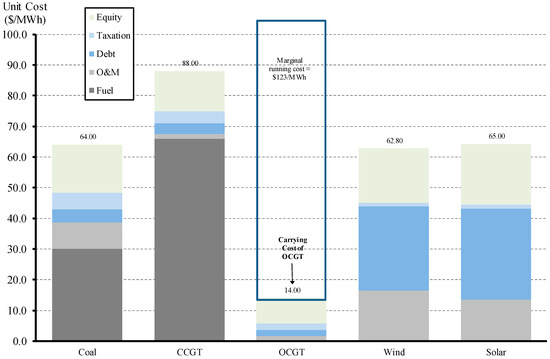
Figure 1.
Generalized plant costs.
3. Model Results and Discussion
3.1. Overview of Power System
The NEMESYS Model has been populated with the plant cost results from Section 2.3, and half-hour load data (using Queensland power system final demand from 2016). From this, multiple scenarios are simulated. A long run (own-price) demand elasticity of −0.30 is applied to all variation cases [49,50,51]. To keep modeling results tractable, the power system is modeled as a single, non-interconnected gross-pool energy-only market. Recall also that the level of government-initiated CfDs are exogenously determined and designed to achieve a certain VRE market share. The base scenario is calibrated with 0% VRE plant (i.e., the power system commences as a thermal system with zero renewable plant), and variation scenarios span up to 40% VRE market share.
Consistent with Equation (6), the objective of the power system model is to minimize resource costs and maximize consumer welfare whilst meeting a reliability constraint of no more than 0.002% unserved energy (i.e., the NEM’s long-standing reliability criteria). To assist interpretation of subsequent results, critical outputs for the two bookend scenarios (i.e., 0% and 40% VRE market share) are presented in Table 2.
Table 2.
Overview of key model results.
Note from Table 2 that the single-region power system has an initial final Energy Demand of 54,717 GWh per annum with peak or Maximum Demand of 9118 MW. Given demand elasticity of −0.30 and the variation in wholesale prices with 40% VRE market share, energy demand and maximum demand rise to 56,386 GWh and 9393 MW, respectively. The opening plant stock is dominated by 6720 MW of coal plant, and in order to meet the reliability constraint (given plant outages) a reserve plant margin of ~11% is necessary. In order to meet a 40% VRE market share, about 3800 MW of wind and 2700 MW of solar PV capacity is added to the plant stock, and given optimal conditions, 2520 MW of coal plant retires. To meet reliability constraints, 800 MW of CCGT plant and 750 MW of OCGT plant is added—albeit operating at relatively low annual capacity factors.
Note also from Table 2 that the power system commences with a dispatch-weighted spot market price of $82.53/MWh and a system average cost of $78.74/MWh. With VRE market share of 40%, total system cost increases to $82.37/MWh whereas the underlying power system price falls to $65.84/MWh—components of this gap being underwritten by government-initiated CfDs with an imputed CO2 value in the range of $25–$35/t. Note that each technology earns a different dispatch-weighted price according to their production profile. In any scenario, OCGT plant earns the highest average spot price (i.e., they increase output at times of high spot prices, and turn off in low spot price periods). Wind plant on the other hand earns a lower average spot price than thermal plant (i.e., coal, CCGT, and OCGT plant) since the stochastic production profile of Australian wind generators has a slight off-peak bias, and in addition, as more wind plant is added to the power system it has an impressing effect on wind’s earned price [6,24,35]. It is worth noting that the dispatch-weighted price of Solar PV plant falls below wind once the technology reaches 7% market share due to the relatively tight correlation amongst all solar PV plant output.
Modeled power system CO2 emissions fall from 53.4 Mt pa to 32.0 Mt pa between the 0% and 40% VRE market share scenarios. Unserved energy in both scenarios is ~0.001% of total load, and thus the plant stock in both scenarios meet the reliability criteria.
3.2. Spot Market Results
Recall that the objective of the current exercise is to analyze the implications of a wide-ranging CfD program on the functioning of an energy-only market, and the hedge market in particular. To model a wide-ranging CfD policy, the installed capacity of wind and solar PV is exogenously increased such that the market share of VRE plant progressively rises to 40% (with model results simulating in 5 percentage point increments). CfD’s are assumed to be initiated by way of auction in order to minimize LCoE outcomes. Based on modeled results, this means that wind and solar PV dominate entry.
Given perfect entry, exit, and exogenously determined levels of government-initiated CfD’s to drive VRE market share, all scenarios are implicitly “long-run dynamic” as measured by the time taken for the capital stock to adjust, rather than specifying a notional time period per se as in [24,35]. The thermal plant stock is therefore assumed to adjust perfectly in that VRE plant entry is accommodated by coal plant retirements (“to make room”, and in line with coal plant financial distress arising from policy-induced VRE plant entry), while moderate levels of CCGT and OCGT plant enter to ensure reliability constraints are met given the intermittent nature of wind and solar PV.
Figure 2 presents the dynamic supply-side adjustment of plant capacity given a policy objective of a 40% VRE market share by way of government-initiated CfDs. Notice in Figure 2 that coal plant capacity reduces from 6720 MW to 4200 MW. Gas-fired capacity increases; CCGT plant commences at 400 MW and rises to 1200 MW while OCGT capacity commences at 3000 MW and rises by a further 750 MW. Consistent with the CfD policy objective, VRE plant increases from 0 MW to 6500 MW, comprising 2700 MW of solar (~15% market share) and 3800 MW of wind (~25% market share).
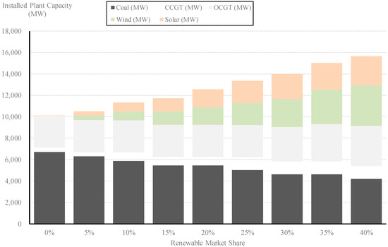
Figure 2.
Installed plant capacity (MW).
Figure 3 shows how plant output adjusts with the addition of wind and solar PV plant gradually reaching a 40% market share. Given limited variations in final demand, supply-side adjustment from VRE plant entry primarily comes from the exit of coal plant. Gas-fired plant capacity continuously rises (see Figure 2) but output responds to both the entry of VRE plant and the exit of coal plant. That is, gas generation (presented as a bar series on the LHS y-axis, and a line series on the RHS y-axis with higher axis resolution to emphasize the variation) provides system flexibility, rising as coal plant exits, and falling as VRE plant increases in output.

Figure 3.
Plant output (GWh).
With perfect plant entry and exit, NEMESYS model results confirm the CfD policy objective can be met with the power system’s spot market producing tractable results. However, what such modeling fails to reveal is an emerging structural shortage in the power system’s financial market, viz. the market for forward hedge contracts used by participants to manage financial risk.
3.3. Financial (Contract) Market Results
Identifying the aggregate supply of hedge contracts within a NEM region is inherently difficult because in a well-functioning power system financial market, there are cross-border trades, and, more than just asset-backed portfolio managers on the sell-side. Proprietary (i.e., non-asset-backed) traders can add substantially to market depth and liquidity. The anonymity of trade makes this notoriously difficult to model (i.e., risk management of market exposures also arises from activity in tangential markets such as the market for weather derivatives, which is similarly excluded from the present analysis).
However, modeling a structural shortage of forward hedge contracts in a single (i.e., non-interconnected) region by is an easier task. The reason for this is that proprietary traders, who add to forward market liquidity, “do not appear out of thin air”. A necessary condition for proprietary trading is an inherent level of forward market liquidity to begin with. Consequently, hedge market analysis need only focus on contract supply from asset-backed traders, which is bounded.
To be perfectly clear on this, if a forward market is illiquid, non-asset-backed traders cannot be relied upon to enter and make-up any shortfall arising from asset-backed traders. Indeed, if forward liquidity begins to contract, proprietary traders will close out their positions and exit the market, thus accelerating any decline in liquidity. The reason for this is axiomatic; as [5] explain, holding-times of various securities is strongly correlated to market liquidity. Again to emphasize, in a forward market characterized by falling liquidity, proprietary traders can be expected to close-out positions, not open new positions, to avoid being caught with unwanted inventory.
Consequently, understanding the total primary supply (i.e., “primary issuance”) of asset-backed forward contracts provides a basis for identifying inherent market liquidity. If the underlying supply or primary issuance of swaps and caps (nominally represented by coal and gas plant respectively) are sufficient relative to maximum demand, then the conditions necessary for trade at “multiples of physical” would appear to exist.
Conversely, if an absolute shortage of primary issuance hedge contracts progressively emerges, then total market liquidity will decelerate, first through the loss of primary supply (i.e., exiting dispatchable coal plant which no longer offers hedges), and then as this initial loss of liquidity becomes obvious, through the progressive exit of proprietary traders as they seek to avoid being caught with unwanted inventory. The combination of this may lead to total financial markets turnover less than 100%, implying some positions are virtually un-hedgeable from within the energy market.
In the analysis that follows, the plant stock outlined in Figure 2 is notionally separated into three rival oligopoly generator portfolios (two at 3520 MW, one at 3080 MW). In the NEMESYS model, individual generation plant availability is determined according to a stochastic binomial distribution with half-hour resolution given plant forced outage rates of ~5%–6%. These generating unit-level data were collated and assembled into joint probability duration curves for each of the three generator portfolios, and from there a 90th percentile confidence limit was identified as the maximum credible supply of asset-backed hedges in a manner consistent with the methodology in [24]. In essence, some plant capacity is withheld from the hedge market for self-insurance against forced plant outages, and to retain some nominal exposure to spot price outcomes. The modeled results that emerge are in turn consistent with the applied hedge market research findings in [20].
Results for Generation Portfolio #1 and Generation Portfolio #3 are presented in Figure 4. Notice that for the 3520 MW Generation Portfolio #1 (and by implication, Generation Portfolio #2 which has an identical plant portfolio) the total potential supply of hedges at the 90th percentile is about 3150 MW, and for the 3080 MW Generation Portfolio #3, total potential supply of hedges is about 2700 MW.
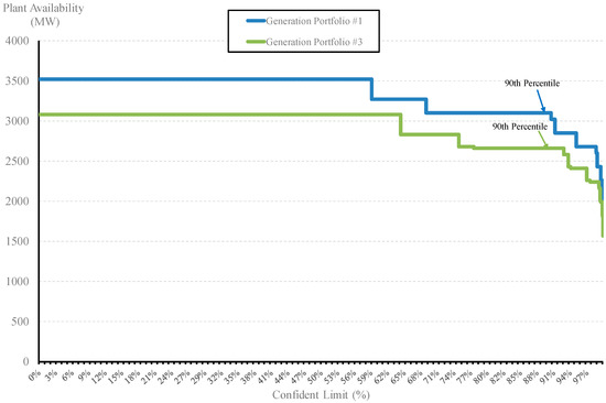
Figure 4.
Primary supply of hedge contracts at 0% renewable market share.
In the model, as VRE plant enters via government-initiated CfDs, various coal generating units exit due to merit-order effects and financial distress. As coal plant exit, some level of gas-fired generation plant enters but as Figure 2 and Figure 3 indicate, the aggregate coal and gas-fired fleet form a shrinking resource vis-à-vis aggregate final demand. Consequently, when the modeling process is undertaken for each of the three Generation Portfolios on a dynamic basis (i.e., as outlined in Figure 2 for VRE = 0%–40%), primary issuance hedge supply begins to decline, and this accelerates as VRE plant entry (by way of CfDs) approaches 40%. The dynamic analysis is presented in Figure 5, which reveals a growing structural shortage of primary issuance hedge contract capacity:
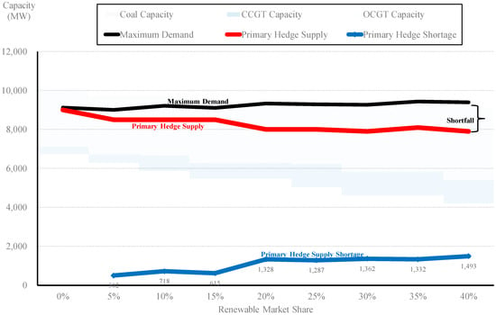
Figure 5.
Primary supply of hedge contracts vs maximum demand (0%–40% VRE).
In Figure 5, the x-axis measures VRE plant market share noting that all plant has been facilitated by government-initiated CfDs (i.e., there are no on-market PPAs). The solid black line series depicts maximum demand, and the solid red line series presents aggregate primary issuance hedge contracts. The gap between the black and red lines highlights the magnitude of any hedge shortfall, also illustrated by solid blue line series—culminating in a hedge market shortfall of ~1500 MW or 16% of final market demand at 40% VRE market share. Note that even with a 5% VRE market share, the impact of government-initiated CfDs produces a non-trivial hedge shortfall if the thermal plant stock adjusts perfectly.
In Figure 5, the dynamic change in plant capacity is also captured by the area chart (grey for coal, dark blue for CCGT plant, and light blue for OCGT plant—essentially a reproduction of Figure 2). In response to the wide-ranging policy of government-initiated CfDs, coal plant contracts from 6700 MW to 4200 MW, while CCGT and OCGT plant capacity expands by 800 MW and 750 MW, respectively. Note that overall there is a net loss of dispatchable plant, and when combined with the extraction of hedge contract capacity from government-initiated CfDs, combines and drives the shortage of primary issuance hedge contracts.
3.4. Hedge Contract Shortages in an Energy-Only Market
The quantitative analysis in Figure 5 in particular revealed that pursuing a wide-ranging program of government-initiated CfDs is likely to produce an “unstable zone” in the forward market for hedge contracts. That is, while the spot market is consistently able to reach equilibrium for any level of VRE output up to 40% market share (given certain dispatch constraints), with government-initiated CfDs the forward hedge market becomes increasingly intractable as thermal plant exits and adjusts. Remaining coal and gas plant are unable to originate sufficient hedge contracts in their own right—as Figure 5 illustrates (recall that coal and gas generators do not hedge 100% of installed capacity due to outage rates and their own desire to maintain some nominal exposure to spot price).
Once a government initiates a wide-ranging program of CfDs, it will have the effect of adding capacity to the spot market which in the short run will lower prices and force coal plant out (consistent with underlying policy objectives), but in the long run will extract 100% of the CfD plant output from the power system’s financial market. Crucially, VRE projects cannot sell their output twice in the forward market.
Consequently, results suggest that a wide-ranging program of government-initiated CfDs is not compatible with the NEM’s energy-only market design. On the contrary, such a policy is likely to collide with the systemic stability of the market. NEM market participants operate in one of the world’s most volatile commodity markets, and access to forward hedge contracts is essential for managing operating risk exposures to sustained critical event price spikes.
Hedge shortage events in energy-only markets with a high VoLL are far more than theory. The South Australian (SA) region of the NEM was known to enter an episode of hedge contract shortages (i.e., hedge contracts <100% of physical) in 2016 and 2017 soon after the final SA coal plant exited (i.e., Northern Power Station during 2016). The surprising sophistication, and level of energy market literacy now displayed by large industrial customers in South Australia explains how the SA market temporarily adjusted. In the short run when hedge contract prices and premiums rose sharply, contract volumes and premiums appear to have been allocated and rationed across the SA power system given segment-level elasticities of demand. That is, prices in the residential consumer segment rose in line with elevated contract premiums. Through discussions with senior NEM policymakers and various industrial customers in SA, it would appear that hedge market shortages were largely absorbed by industrial customers in the short run, with a typical strategy being to secure some minimum level of hedging and run the balance of manufacturing load to the spot market (while keeping a close eye on exposed load to pre-dispatch prices).
The SA hedge market shortage was ultimately caused by the sudden and uncoordinated exit of coal plant—replacement hedge capacity is slowly being rebuilt through various new entrant VRE plant, battery storage, and gas turbines. But if the new VRE entrants were underwritten by way of government-initiated CfDs, it is not immediately obvious how such a shortfall could be rebuilt.
A wide-ranging program of government-initiated CfDs may adversely impact the residential and SME business market. The effect of extracting hedge contract capacity from the forward market may, in time, weigh heavily on retail competition. Large vertical retailers can be expected to manage positions using a combination of physical plant and forward markets—and these large utility firms have the financial capacity to allocate resources seamlessly between the two. But 2nd tier non-integrated retailers do not have the same financial resources and may in the event be inadvertently foreclosed by a wide-ranging government policy of CfDs as financial market liquidity deteriorates and hedge shortages bind. At this point, retail-level consumer pricing can also be expected to be adversely impacted through less competition.
And, un-hedgeable positions may introduce risks to the systemic stability of power market more generally. If a sufficiently large utility experienced financial distress due to excessive exposure to VoLL events because they were not able to allocate resources between physical plant and forward markets quickly enough, it could lead to cascading failures across the power market economy; unlike Australian financial institutions which can access lender of last resort facilities with the Commonwealth Government, there is no centralized financial backstop for Australia’s organized energy markets.
3.5. Are Hedge Shortages Inevitable with Rising VRE Plant?
Modeling results in Section 3.3 explicitly assume VRE plant enters exclusively by way of government-initiated CfDs, and that these CfDs crowd-out on-market (bilateral) private sector PPAs. The result was a shortage of hedges. A logical question that follows is whether hedge contract shortages are inevitable in a world of rising VRE market share and coal plant exit regardless of how entry occurs—whether by government-initiated CfDs or by on-market PPAs amongst NEM market participants? The short answer is no. Results in Figure 5 would look different if VRE plant was able to provide its output, in spite of intermittency, into the hedge books of market participants (as is the case under a certificate-based renewable portfolio standard). That is, participants and portfolio traders can synthetically (or physically) reconstruct firm hedge contract positions by combining run-of-plant PPAs with dispatchable plant (e.g., incumbent coal, and existing or new, CCGT, OCGT, pumped-hydro, battery storage) and rely on gains from exchange in the spot market to balance positions on a risk-adjusted basis. Whether forward hedge market demand ultimately clears without materially higher reserve plant margins in the long run is an open question.
3.6. Not A Short-Run Problem
The use of government-initiated CfDs will not create hedge contract shortages in the short run. It is a long run problem [24,35]. If thermal plant fails to exit or thermal plant capacity remains above efficient levels, shortages in the hedge market are unlikely to appear. Indeed, in the short run government-initiated CfDs may well result in consumers benefiting from a surplus of hedge contract capacity (i.e., if thermal plant does not exit they are still available to supply hedge contracts), and short-run prices will be lower reflecting merit-order effects of adding VRE plant to the power system.
However, and to be clear, as coal plant exits the opposite occurs as evidenced by the South Australian NEM region in 2016–2017. Thermal plant must exit due to inevitable financial distress caused by VRE plant entry at-scale. And the exit of coal plant causes spot prices to rebound. Furthermore, in such a CfD scenario spot prices will rebound just as hedge contract shortages appear; thus, consumers would be unable to hedge against the very reason for hedging in the first place—viz. the risk of sharply rising wholesale market prices. And in the modeling results in Section 3.3, the reason consumers cannot fully hedge in forward markets is because hedge capacity has been extracted through a wide-ranging program of government-initiated CfDs.
3.7. Validity of Government-Initiated CfD Reallocation Mechanisms
One reviewer queried whether, to remain consistent with the energy-only market design, government-initiated CfD “receipts and payments” could be allocated to energy retailers on a pro-rata basis as is done in Great Britain’s net pool market. The line of reasoning would be that energy retailers could impute a hedge position based on the output of the VRE plant portfolio contracted by the government.
This would represent a poor outcome. When energy retailers enter into bilateral PPAs under a renewable portfolio standard or emissions obligation, the terms and conditions are invariably non-vanilla and designed to suit the allocation of risk between VRE producer and energy retailer, and, with a known project, project location and real-time project-specific output and associated constraints. Under a government reallocation, the shareholders of energy retailers would be forced to digest a “blind hedge book” and simultaneously lose control over the timing, cost, location, and magnitude of VRE plant commitments. How this could add to market efficiency is not immediately obvious.
Another reviewer queried whether governments could initiate CfDs, and then on-sell the CfD on a project-by-project basis in the open market at market rates (i.e., effectively creating a secondary market to recycle CfD’s as a PPA, and in the process crystalize taxpayer profits or losses on each transaction). This is a plausible solution to the modeling results outlined in Section 3.3. But apart from adding a layer of transaction costs into the NEM and using scarce government balance sheet resources for needless intermediation, such a policy strategy implicitly presumes a central government agency will purchase more efficiently than an entire energy market comprising no less than 50 highly sophisticated organizations. A key reason energy markets exist is government failures in the central planning of power systems. The better view is for government to set the policy objective and policy targets (i.e., renewable portfolio standard or emissions obligation), and let the market deliver the policy objective and allocate the various power system financial and operating risks to those best able to manage them.
4. Conclusions
Australia has an international obligation to reduce its CO2 emissions under the Paris Agreement, and Australia’s NEM is a CO2-intensive power system by OECD standards [52]. In this article, a requirement to lower the CO2 intensity of the NEM has been taken as an exogenous policy constraint in the form of a 40% VRE market share. The purpose of this modeled constraint was not to test optimal levels or the composition of VRE plant, nor the structural adjustment task and welfare implications of exiting coal plant at-scale. The specific line of inquiry was to determine whether the wide-spread use of off-market government-initiated CfDs to achieve higher VRE and lower CO2 emissions is compatible with the NEM’s energy-only market design.
Australia’s renewable energy target (i.e., renewable portfolio standard) required that energy retailers meet a 20% renewable market share by 2020. The certificated scheme will be comfortably met—by 2018 the NEM had 8000 MW of new VRE plant (5000 MW wind, 2800 MW solar) and a further 5500 MW was under construction as at the start of 2019 (2500 MW wind and 3000 MW solar). On-market transactions had delivered more than $20 billion of investment without any need for government involvement or intermediation beyond setting the policy framework. The market was given a target, and market participants (i.e., utilities, investors, and customers) delivered the capacity.
Used carefully, CfDs present policymakers with a reliable tool which can be used to overcome an array of market failures, including those associated with missing or incomplete markets (including emergency plant for security of supply reasons, certain positive, or negative externalities including CO2 emissions, R&D and externalities arising from first-of-a-kind commercialization investments). In the NEM, CfDs have been used selectively and effectively by state governments to “prime” emerging markets, navigate Commonwealth Government policy discontinuity, with material on-market transactions following. The Australian Capital Territory government CfDs pioneered nominal-price transactions, the Queensland government’s CfDs led to more than 1900 MW of follow-on solar PV projects, and the SA government’s semi-CfD for battery storage in has since resulted in more than a dozen battery projects either under active development or commitment. From a project execution perspective, the effectiveness of government-initiated CfDs are unquestionable.
But in an energy-only market setting, government-initiated CfDs must be used judiciously because they introduce “quasi-market participants” who do not respond to spot market signals, and do not participate in forward markets at all. Quasi-market participants are indifferent or substantially immune from future outcomes in spot and forward markets. This can result in plant entry that is poorly timed, poorly sized, poorly located, and above all, poorly motivated to respond to the electricity and frequency control ancillary service spot price signals which keep the power system operating in a stable manner.
CfD plant also benefits from otherwise unachievable credit metrics owing to a taxpayer-financed and credit-wrapped CfD instrument—with the risks transferred to taxpayers. Prima facie this may deliver lower project specific LCoE’s, but this is only because risk has been transferred to taxpayers (which is not costless), and whether this is an efficient allocation and use of government balance sheet capacity is, in my opinion, questionable. A wide-ranging program of government-initiated CfDs can be expected to crowd-out on-market rival merchant/bilateral investments.
If there is an upside to the present analysis, it is that the number of alternate policy instruments available to government to achieve policy objectives has expanded very rapidly [53]. A wide array of policy instruments exist to deal with the market failures which CfDs are intended to remedy; renewable energy policy objectives can be achieved by an emissions obligation or well-designed renewables portfolio standard [48]; the need for emergency capacity can be (and in the NEM recently has been) dealt with by establishing minimum exit notification periods for plant intending to exit the system; resource adequacy (i.e., adequate plant capacity including an appropriate reserve plant margin) can be maintained by ensuring the level of VoLL remains appropriate or by pursuing reliability obligations if this becomes necessary. All of these options work with an energy-only market design, including the forward market for contracts.
Throughout most of 2018, Australian policymakers developed a policy known as the National Energy Guarantee which had two embedded policy mechanisms for energy retailers to comply with; (i) an emissions obligation which was consistent with Australia’s international CO2 commitments under the Paris Agreement, and (ii) a reliability obligation which was consistent with the NEM’s reliability criteria and was designed to ensure resource adequacy. The former was designed to encourage hedge contract activity with new renewable projects, and the latter was designed to be acquitted via ensuring adequate forward contracts were committed—both mechanisms were thus designed to add to liquidity rather than detract from it.
In contrast, as quantitative results and analysis in this article explain, a wide-ranging program of government-initiated CfDs can be expected to impair market efficiency in an energy-only market setting. While adding to buy-side liquidity, government-initiated CfDs replace on-market transactions and thus subtract from sell-side liquidity, and this matters in loosely-interconnected energy-only markets because as coal plant exits, primary issuance hedge contract shortages become predictable. Shortages in the forward markets may harm consumer welfare by raising contract premiums—the primary input into consumer tariffs—and by forcing the most price-elastic industrial customers into accepting spot market exposures, which at best disrupts manufacturing efficiency. Further, CfD-driven hedge market shortages may unintentionally foreclose non-integrated 2nd tier retailers—deeming such a program of government-initiated CfDs to be (unintentionally) anti-competitive. Consequently, the National Energy Guarantee or an equivalent suite of policies seems a better place for Australian policymakers to focus on.
Funding
This research received no external funding.
Conflicts of Interest
The author declares no conflicts of interest.
Abbreviations
The following abbreviations are used in this manuscript:
| AUD | Australian Dollars |
| CCGT | Combined Cycle Gas Turbine |
| CfD | Contract for Differences |
| CO2 | Carbon Dioxide |
| LCoE | Levelized Cost of Electricity |
| NEM | National Electricity Market |
| OCGT | Open Cycle Gas Turbine |
| O&M | Operations & Maintenance |
| PV | Photovoltaic |
| RET | Renewable Energy Target |
| VoLL | Value of Lost Load |
| VRE | Variable Renewable Energy (i.e., wind and solar PV) |
Appendix A
The purpose of the PF model is to produce plant cost estimates for various generating technologies. The PF model is essentially a dynamic, multi-period post-tax discounted cash flow optimization model which solves for multiple generating technologies, business combinations, and revenue possibilities through simultaneous convergent price, debt-sizing, taxation and equity return variables. These outputs are similar in nature to levelized cost estimates but with a level of detail beyond the typical LCoE model because corporate or project financing, credit metrics and taxation constraints are co-optimized. Model logic, derived in [48,54], is as follows:
Costs increase annually by a forecast general inflation rate (CPI). Prices escalate at a discount to CPI. Inflation rates for revenue streams and cost streams in period (year) j are calculated as follows:
Energy output from each plant (i) in each period (j) is a key variable in driving revenue streams, unit fuel costs and variable operations and maintenance costs. Energy output is calculated by reference to installed capacity , capacity utilisation rate for each period j. Plant auxiliary losses arising from on-site electrical loads are deducted.
Electricity price for the ith plant is calculated in year one and escalated per Eq. (A1). Thus revenue for the ith plant in each period j is defined as follows:
As outlined above, plant marginal running costs are a key variable and used extensively in NEMESYS-PF. In order to define marginal running costs, the thermal efficiency for each generation technology needs to be defined. The constant term “3600” is divided by to convert the efficiency result from % to kJ/kWh (i.e., the derivation of the constant term 3600 is: 1 Watt = 1 Joule per second and hence 1 Watt Hour = 3600 Joules). This is then multiplied by raw fuel commodity cost . Variable operations and maintenance costs , where relevant, are added which produces a pre-carbon short run marginal cost. Under conditions of externality pricing , the CO2 intensity of output needs to be defined. Plant carbon intensity is derived by multiplying the plant heat rate by combustion emissions and fugitive CO2 emissions . Marginal running costs in the jth period is then calculated by the product of short run marginal production costs by generation output and escalated at the rate of .
Fixed operations and maintenance costs of the plant are measured in $/MW/year of installed capacity and are multiplied by plant capacity and escalated.
Earnings before interest tax depreciation and amortization (EBITDA) in the jth period can therefore be defined as follows:
Capital costs for each plant i are overnight capital costs and incurred in year 0. Ongoing capital spending for each period j is determined as the inflated annual assumed capital works program.
Plant capital costs give rise to tax depreciation () such that if the current period was greater than the plant life under taxation law (L), then the value is 0. In addition, also gives rise to tax depreciation such that:
From here, taxation payable at the corporate taxation rate is applied to less interest on loans later defined in (16), less . To the extent results in non-positive outcome, tax losses are carried forward and offset against future periods.
The debt financing model computes interest and principal repayments on different debt facilities depending on the type, structure, and tenor of tranches. There are two types of debt facilities—(a) corporate facilities (i.e., balance-sheet financings) and (2) project financings. Debt structures include semi-permanent amortizing facilities and bullet facilities.
Corporate facilities involve 3- and 7-year money raised with an implied “BBB” credit rating. With project financings, two facilities are modeled. The first facility is nominally a 3-year bullet requiring interest-only payments after which it is refinanced with consecutive amortizing facilities and fully amortized over a 25-year period. The second facility commences with a tenor of 7 years as an amortizing facility, again set within a semi-permanent structure with a nominal repayment term of 25 years. The decision tree for the two tranches of debt is the same, so for the debt tranche where = 1 or 2, the calculation is as follows:
refers to the total amount of debt raised for the project. The split (S) of the debt between each facility refers to the manner in which debt is apportioned to each tranche. In the model, 35% of debt is assigned to Tranche 1 and the remainder to Tranche 2. Principal refers to the amount of principal repayment for tranche T in period j and is calculated as an annuity:
In (A12), is the relevant interest rate swap (3 yrs or 7 yrs) and is the credit spread or margin relevant to the issued debt tranche. The relevant interest payment in the jth period is calculated as the product of the (fixed) interest rate on the loan by the amount of loan outstanding:
Total debt outstanding , total Interest and total principle for the ith plant is calculated as the sum of the above components for the two debt tranches in time j. For clarity, loan drawings are equal to in year 1 as part of the initial financing and are otherwise 0.
One of the key calculations is the initial derivation of . This is determined by the product of the gearing level and the overnight capital cost . Gearing levels are formed by applying a cash flow constraint based on credit metrics applied by project banks and capital markets. The variable in the PF model relates specifically to the legal structure of the business and the credible capital structure achievable. The two relevant legal structures are vertically integrated (VI) merchant utilities (using “BBB” rated corporate facilities) and independent power producers using project finance (PF).
The variables and are exogenously determined by credit rating agencies. Values for are exogenously determined by project banks and depend on technology (i.e., thermal vs. renewable) and the extent of energy market exposure, that is whether a power purchase agreement exists or not. For clarity, is “funds from operations” while and are the debt service cover ratio and loan life cover ratios. Debt drawn is:
At this point, all of the necessary conditions exist to produce estimates of generalized long run marginal costs of the various power generation technologies. The relevant equation to solve for the price given expected equity returns whilst simultaneously meeting the binding constraints of and or given the relevant business combinations. The primary objective is to expand every term which contains . Expansion of the EBITDA and tax terms is as follows:
The terms are then rearranged such that only the term is on the left-hand side of the equation:
Let
The model then solves for such that:
Table A1.
Corporate Finance Assumptions.
Table A1.
Corporate Finance Assumptions.
| Coal & Gas | Wind & Solar | ||
|---|---|---|---|
| Debt Sizing Constraints | Debt Sizing Constraints | ||
| FFO/I (times) | 5 | DSCR (times) | 1.35 |
| FFO/D (times) | 3 | LLCR (times) | 1.35 |
| Gearing Limit (%) | 40.0 | Gearing Limit (%) | 70.0 |
| Default (times) | 1.10 | ||
| Corporate “BBB” Bonds | Project Finance Facilities | ||
| Tranche 1 (Bullet) (Yrs) | 5 | Tranche 1 (Bullet) (Yrs) | 5 |
| Tranche 1 Refi (Yrs) | 13–20 | Tranche 1 Refi (Yrs) | 13–20 |
| Tranche 2 (Amort.) (Yrs) | 7 | Tranche 2 (Amort.) (Yrs) | 7 |
| Notional amortization (Yrs) | 18–25 | Notional amortization (Yrs) | 18–25 |
| BBB Bond Pricing | Project Finance Facilities-Pricing | ||
| Tranche 1 (%) | 3.60 | Tranche 1 Swap (%) | 2.55 |
| Tranche 1 Margin (bps) | 105 | Tranche 1 Margin (bps) | 200 |
| Tranche 2 (%) | 3.97 | Tranche 2 Swap (%) | 2.68 |
| Tranche 2 Margin (bps) | 129 | Tranche 2 Margin (bps) | 220 |
| Tranche 1 (%) | 3.60 | Tranche 1 (%) | 4.55 |
| Tranche 2 (%) | 3.97 | Tranche 2 (%) | 4.88 |
| Tranche 1&2 Refi (%) | 3.97 | Tranche 1&2 Refi (%) | 4.88 |
| Post Tax Equity Coal (%) | 12.0 | Post Tax Equity (%) | 10.0 |
| Post Tax Equity Gas (%) | 12.0 | ||
References
- Nong, D. A general equilibrium impact study of the Emissions Reduction Fund in Australia by using a national environmental and economic model. J. Clean. Prod. 2019, 216, 422–434. [Google Scholar] [CrossRef]
- Simshauser, P.; Tiernan, A. Climate change policy discontinuity and its effects on Australia’s National Electricity Market. Aust. J. Publ. Admin. 2019, 78, 17–36. [Google Scholar] [CrossRef]
- Wild, P. Determining commercially viable two-way and one-way ‘Contract-for-Difference’ strike prices and revenue receipts. Energy Policy 2017, 110, 191–201. [Google Scholar] [CrossRef]
- Bunn, D.; Yusupov, T. The progressive inefficiency of replacing renewable obligation certificates with Contracts-for-Differences in the UK electricity market. Energy Policy 2015, 82, 298–309. [Google Scholar] [CrossRef]
- Goldstein, M.; Hotchkiss, E. Providing Liquidity in an Illiquid Market: Dealer Behavior in U.S. Corporate Bonds. July 2018. Available online: https://papers.ssrn.com/sol3/papers.cfm?abstract_id=2977635 (accessed on 5 May 2018).
- Hirth, L.; Ueckerdt, F.; Edenhofer, O. Why wind is not coal: On the economics of electricity generation. Energy J. 2016, 37, 1–27. [Google Scholar] [CrossRef]
- Hansen, C. Improving hedge market arrangements in New Zealand. In Proceedings of the 6th Annual National Power New Zealand Conference, Auckland, New Zealand, 30 March 2004. [Google Scholar]
- Chao, H.; Oren, S.; Wilson, R. Re-evaluation of Vertical Integration and Unbundling in Restructured Electricity Markets. In Competitive Electricity Markets: Design, Implementation, Performance; Sioshansi, F.P., Ed.; Elsevier: Oxford, UK, 2008. [Google Scholar]
- Finon, D. Investment risk allocation in decentralised markets: The need of long-term contracts and vertical integration. OPEC Energy Rev. 2008, 32, 150–183. [Google Scholar] [CrossRef]
- Meade, R.; O’Connor, S. Comparison of long-term contracts and vertical integration in decentralised electricity markets. In Competition, Contracts and Electricity Markets: A new perspective; Glachant, J.M., Finon, D., De Hauteclocque, A., Eds.; Edward Elgar Publishing: Cheltenham, UK, 2011. [Google Scholar]
- Finon, D. Investment and Competition in Decentralized Electricity Markets: How to Overcome Market Failure by Market Imperfections? In Competition, Contracts and Electricity Markets: A new perspective; Glachant, J.M., Finon, D., De Hauteclocque, A., Eds.; Edward Elgar Publishing: Cheltenham, UK, 2011. [Google Scholar]
- Meyer, R. Vertical economies and the costs of separating electricity supply—A review of theoretical and empirical literature. Energy J. 2012, 33, 161–185. [Google Scholar] [CrossRef]
- Nelson, J.; Simshauser, P. Is the merchant power producer a broken model? Energy Policy 2013, 53, 298–310. [Google Scholar] [CrossRef][Green Version]
- Newbery, D. Missing money and missing markets: Reliability, Capacity Auctions and Interconnectors. Energy Policy 2015, 94, 401–410. [Google Scholar] [CrossRef]
- Newbery, D. Tales of Two Islands—Lessons for EU Energy Policy from Electricity Market Reforms in Britain and Ireland. Energy Policy 2016, 105, 597–607. [Google Scholar] [CrossRef]
- Grubb, M.; Newbery, D. UK Electricity Market Reform and the Energy Transition. Energy J. 2018, 39, 1–25. [Google Scholar] [CrossRef]
- Newbery, D. Market Design; EPRG Working Paper 515; University of Cambridge: Cambridge, UK, 2006. [Google Scholar]
- Green, R. Market power mitigation in the UK power market. Util. Policy 2006, 14, 76–89. [Google Scholar] [CrossRef]
- Chester, L. The conundrums facing Australia’s National Electricity Market. Econ. Pap. 2006, 25, 262–277. [Google Scholar] [CrossRef]
- Anderson, E.; Hu, X.; Winchester, D. Forward contracts in electricity markets: The Australian experience. Energy Policy 2007, 35, 3089–3103. [Google Scholar] [CrossRef]
- Howell, B.; Meade, R.; O’Connor, S. Structural separation versus vertical integration: Lessons for telecommunications from electricity reforms. Telecommun. Policy 2010, 34, 392–403. [Google Scholar] [CrossRef][Green Version]
- Simshauser, P. Vertical integration, credit ratings and retail price settings in energy-only markets: Navigating the Resource Adequacy problem. Energy Policy 2010, 38, 7427–7441. [Google Scholar] [CrossRef][Green Version]
- Pollitt, M.; Anaya, K. Can current electricity markets cope with high shares of renewables? A comparison of approaches in Germany, the UK and the State of New York. Energy J. 2016, 37, 69–88. [Google Scholar] [CrossRef]
- Simshauser, P. On intermittent renewable generation & the stability of Australia’s National Electricity Market. Energy Econ. 2018, 72, 1–19. [Google Scholar]
- Department for Business Energy & Industrial Strate. Electricity Market Reform: Contracts for Difference; UK Government: London, UK, 2015.
- Department of Environment Land Water and Planning. Victorian Renewable Energy Auction Scheme: Consultation Paper; Victorian State Government: Melbourne, Australia, 2015.
- Environment, Planning and Sustainable Development. How Do the ACT’s Renewable Energy Reverse Auctions Work? ACT Government: Canberra, Australia, 2016.
- Queensland Renewable Energy Expert Panel. Credible Pathways to A 50% Renewable Energy Target for Queensland; Queensland Government: Brisbane, Australia, 2016.
- Department of the Environment and Energy. Underwriting New Generation Investments—Call for Registrations of Interest; Commonwealth of Australia: Canberra, Australia, 2018.
- Kozlov, N. Contract for difference: Risks faced by generators under the new renewables support scheme in the UK. J. World Energy Bus. Law 2014, 7, 282–286. [Google Scholar] [CrossRef]
- Onifade, T. Hybrid renewable energy support policy in the power sector: The contracts for difference and capacity market case study. Energy Policy 2016, 95, 390–401. [Google Scholar] [CrossRef]
- Joskow, P. Comparing the costs of intermittent and dispatchable electricity generating technologies. American Econ. Rev. 2011, 100, 238–241. [Google Scholar] [CrossRef]
- Mills, A.; Wiser, R. Changes in the Economic Value of Variable Generation At High Penetration Levels: A Pilot Case Study of California; LBNL-5445E; Lawrence Berkeley National Laboratory: Berkeley, CA, USA, 2012. [Google Scholar]
- Edenhofer, O.; Hirth, L.; Knopf, B.; Pahle, M.; Schlomer, S.; Schmid, E.; Ueckerdt, F. On the economics of renewable energy sources. Energy Econ. 2013, 40, S12–S23. [Google Scholar] [CrossRef]
- Hirth, L. The market value of variable renewables: The effect of solar & wind power variability on their relative price. Energy Econ. 2013, 38, 218–236. [Google Scholar]
- MacGill, I. Electricity market design for facilitating the integration of wind energy: Experience and prospects with the Australian National Electricity Market. Energy Policy 2010, 38, 3180–3191. [Google Scholar] [CrossRef]
- Nicolosi, M. The economics of renewable electricity market integration. An empirical and model-based analysis of regulatory frameworks and their impacts on the power market. Ph.D. Thesis, University of Cologne, Cologne, Germany, 2012. [Google Scholar]
- Green, R.; Staffell, I. Electricity in Europe: Exiting fossil fuels? Oxford Rev. Econ. Policy 2016, 32, 282–303. [Google Scholar] [CrossRef]
- Nelson, T.; Simshauser, P.; Nelson, J. Queensland solar feed-in tariffs and the merit-order effect: Economic benefit, or regressive taxation and wealth transfers? Econ. Anal. Policy 2012, 42, 277–301. [Google Scholar] [CrossRef]
- Joskow, P. Symposium on Capacity Markets. Econ. Energy Environ. Policy 2013, 2, v–vi. [Google Scholar]
- Sensfuβ, F.; Ragwitz, M.; Genoese, M. The merit-order effect: A detailed analysis of the price effect of renewable electricity generation on spot market prices in Germany. Energy Policy 2008, 36, 3086–3094. [Google Scholar] [CrossRef]
- Forrest, S.; MacGill, I. Assessing the impact of wind generation on wholesale prices and generator dispatch in the Australian National Electricity Market. Energy Policy 2013, 59, 120–132. [Google Scholar] [CrossRef]
- Cludius, J.; Forrest, S.; MacGill, I. Distributional effects of the Australian Renewable Energy Target (RET) through wholesale and retail electricity price impacts. Energy Policy 2014, 71, 40–51. [Google Scholar] [CrossRef]
- Bell, W.; Wild, P.; Foster, J.; Hewson, M. Wind speed and electricity demand correlation analysis in the Australian National Electricity Market: Determining wind turbine generators’ ability to meet electricity demand without energy storage. Econ. Anal. Policy 2015, 48, 182–191. [Google Scholar] [CrossRef][Green Version]
- Bell, W.; Wild, P.; Foster, J.; Hewson, M. Revitalising the wind power induced merit-order effect to reduce wholesale and retail electricity prices in Australia. Energy Econ. 2017, 67, 224–241. [Google Scholar] [CrossRef]
- Felder, F. Examining electricity price suppression due to renewable resources and other grid investments. Elec. J. 2011, 24, 34–46. [Google Scholar] [CrossRef]
- Bushnell, J. Building Blocks: Investment in Renewable and Non-Renewable Technologies. In Harnessing Renewable Energy in Electric Power Systems: Theory, Practice, policy; Moselle, B., Padilla, J., Schmalensee, R., Eds.; Routledge: Berkley, CA, USA, 2010. [Google Scholar]
- Simshauser, P.; Gilmore, J. On Entry Cost Dynamics in Australia’s National Electricity Market; EPRG Working Paper No.1841; University of Cambridge: Cambridge, UK, 2018. [Google Scholar]
- Australian Energy Market Operator. Electricity Demand Forecasting Methodology Information Paper; AEMO Publication: Melbourne, Australia, 2019. [Google Scholar]
- Narayan, K.; Smyth, R. The residential demand for electricity in Australia: An application of the bounds testing approach to cointegration. Energy Policy 2005, 33, 467–474. [Google Scholar] [CrossRef]
- Fan, S.; Hyndman, R. The price elasticity of electricity demand in South Australia. Energy Policy 2011, 39, 709–3719. [Google Scholar] [CrossRef]
- Grattan Institute. Commonwealth Orange Book 2019; Grattan Institute Publication: Melbourne, Australia, 2019. [Google Scholar]
- Peters, B. Governance: A Garbage Can Perspective; Institute for Advanced Studies: Vienna, Austria, 2002. [Google Scholar]
- Simshauser, P.; Ariyaratnam, J. What is normal profit for power generation? J. Financ. Econ. Policy 2014, 6, 152–178. [Google Scholar] [CrossRef]


© 2019 by the author. Licensee MDPI, Basel, Switzerland. This article is an open access article distributed under the terms and conditions of the Creative Commons Attribution (CC BY) license (http://creativecommons.org/licenses/by/4.0/).