Article

An Efficient Method to Predict Compressibility Factor of Natural Gas Streams

by
Vassilis Gaganis
1,†,
Dirar Homouz
2,†,
Maher Maalouf
3,*,
Naji Khoury
4 and
Kyriaki Polychronopoulou
5,*,‡
1
Mining and Metallurgical Engineering, National Technical University of Athens, Athens 157 73, Greece
2
Applied Mathematics and Sciences, Khalifa University, Abu Dhabi, P.O. Box 127788, United Arab Emirates
3
Industrial and Systems Engineering, Khalifa University, Abu Dhabi, P.O. Box 127788, United Arab Emirates
4
Civil and Environmental Engineering, Notre Dame University Louaize, Beirut, P.O. Box 72, Zouk Mikael, Lebanon
5
Mechanical Engineering, Khalifa University, Abu Dhabi, P.O. Box 127788, United Arab Emirates
*
Authors to whom correspondence should be addressed.
These authors contributed equally to this work.
Current address: Center for Catalysis and Separations, Khalifa University, Abu Dhabi, P.O.Box 127788, United Arab Emirates.
Energies 2019, 12(13), 2577; https://doi.org/10.3390/en12132577
Submission received: 17 April 2019 / Revised: 17 May 2019 / Accepted: 24 May 2019 / Published: 4 July 2019
(This article belongs to the Section I: Energy Fundamentals and Conversion)

Abstract

:
The gas compressibility factor, also known as the deviation or Z-factor, is one of the most important parameters in the petroleum and chemical industries involving natural gas, as it is directly related to the density of a gas stream, hence its flow rate and isothermal compressibility. Obtaining accurate values of the Z-factor for gas mixtures of hydrocarbons is challenging due to the fact that natural gas is a multicomponent, non-ideal system. Traditionally, the process of estimating the Z-factor involved simple empirical correlations, which often yielded weak results either due to their limited accuracy or due to calculation convergence difficulties. The purpose of this study is to apply a hybrid modeling technique that combines the kernel ridge regression method, in the form of the recently developed Truncated Regularized Kernel Ridge Regression (TR-KRR) algorithm, in conjunction with a simple linear-quadratic interpolation scheme to estimate the Z-factor. The model is developed using a dataset consisting of 5616 data points taken directly from the Standing–Katz chart and validated using the ten-fold cross-validation technique. Results demonstrate an average absolute relative prediction error of 0.04%, whereas the maximum absolute and relative error at near critical conditions are less than 0.01 and 2%, respectively. Most importantly, the obtained results indicate smooth, physically sound predictions of gas compressibility. The developed model can be utilized for the direct calculation of the Z-factor of any hydrocarbon mixture, even in the presence of impurities, such as N 2 , CO 2 , and H 2 S, at a pressure and temperature range that fully covers all upstream operations and most of the downstream ones. The model accuracy combined with the guaranteed continuity of the Z-factor derivatives with respect to pressure and temperature renders it as the perfect tool to predict gas density in all petroleum engineering applications. Such applications include, but are not limited to, hydrocarbon reserves estimation, oil and gas reservoir modeling, fluid flow in the wellbore, the pipeline system, and the surface processing equipment.

1. Introduction

Fluid properties are directly involved in all flow and volumetric calculations in the upstream and downstream zones of the petroleum industry. Density and its change over pressure, vaporization, or condensation ratios, as well as kinetic properties such as viscosity all affect the obtained results [1,2,3,4]. For the case of natural gas, various calculations need to be run including the estimation of hydrocarbon reserves in a reservoir, the study of the gas flow in the reservoir and the wellbore, and its thermodynamic behavior through the pipelining system until its arrival at the sales point and further transportation to the end user, whereas the latter could be a home user, a plant, or an electric power generation unit. The accurate determination of gas density is of utmost importance, directly related to the conversion of flow rates from line conditions to standard ones where rates are commonly reported. Moreover, the rate of change of density with pressure under constant temperature, known as isothermal compressibility, is related to the accumulation or withdrawal of mass in a control volume such as a reservoir when that volume is depleted and pressure undergoes reduction.
Although natural gas is a complex multi-component mixture with methane being the major compound and other compounds such as nitrogen, carbon dioxide, ethane, propane, and heavier hydrocarbons at lower concentrations [5,6], for the special case of near surface conditions, it can be treated as an ideal one. Therefore, its thermodynamic behavior is governed by the ideal gas Equation of State (EoS) V m = R T p , where V m denotes molar volume; hence, density ρ and compressibility c at pressure p and at temperature T are given respectively by:
ρ = p M R T
c = 1 V d V d p = 1 p
where M stands for the fluid’s molar mass. To handle conditions far from the atmospheric one, the above definition needs to be extended by introducing the deviation factor Z, also known as the compressibility factor, not to be confused with isothermal compressibility, such that V m = Z R T p . In that case, the density and compressibility of the gas are given by:
ρ = p M Z R T
and:
c = 1 V d V d p = 1 p 1 Z d Z d p
respectively. From a thermodynamic perspective, the Z-factor basically describes the deviation between real gas and ideal gas behavior. There are a number of accurate equations of state providing estimates of the Z-factor; among them are the Soave–Redlich–Kwong (SRK) [7], the Peng–Robinson (PR) [8], the Lee–Kesler EoS [9], and the Zudkevitch–Joffe–Redlich–Kwong (ZJRK) ones [10]. Research has been published also for the calculation of the virial coefficients of the EoS [11]. Clearly, all EoS-based methods to predict the Z-factor need an accurate description of the gas composition and characterization of all its components. This last step can be very tedious, as it involves estimation of properties’ components such as critical values, acentric factors, and binary interaction coefficients.
Another group of methods takes advantage of the corresponding states principle according to which fluids at the same reduced pressure and temperature exhibit very close compressibility factor values. Reduced conditions are defined by p r = p p c and T r = T T c , respectively, where p c and T c denote the mixture’s critical pressure and temperature, respectively. The most pronounced method to compute the Z-factor by this approach is the use of the industry-standard Standing–Katz (S-K) chart [5], which provides the Z-factor of natural gas as a function of its reduced properties. This chart is known to perform surprisingly accurately for hydrocarbon mixtures, although it has been generated by using experimental data from a very limited dataset. This chart, originally generated in the early 1940s, is valid for T r values in [ 1.05 , 3.0 ] and p r values up to 15. Later, it was extended [12] up to p r equal to 30 only for a narrower range of reduced temperatures, i.e., T r [ 1.4 , 2.8 ] . When impurities are present, the correction method of Wichert and Aziz [13] needs to be utilized. Various mixing rules are available to estimate mixture’s T c and p c when the composition and the critical properties of the gas components are known. The methods of Kay [14], Stewart–Burkhardt–Voo (SBV) [15] and Sutton [16] are the most widely used. When either the composition or the gas components’ critical properties are unknown, the S-K chart is still applicable by utilizing the pseudo-critical properties p p c and T p c , respectively. The latter can be computed from correlations of the specific gravity [17], thus leading to the estimation of the Z-factor by means of the pseudo-reduced values defined by p p r = p / p p c and T p r = T / T p c . For the sake of simplicity, we will use p r and T r to denote both reduced and pseudo-reduced pressure and temperature in the following sections.
To facilitate the use of computers, the S-K chart has been fitted by various correlations, which can be distinguished into two categories. Firstly, the iterative ones require repeated calculations to solve a non-linear algebraic equation, the root of which is the Z-factor or a direct function of that. The methods of Hall and Yarborough (H-Y) [18], as well as that of Dranchuk and Abu Kassem (DAK) [19] are the most pronounced ones in this category. Secondly, explicit correlations are available for directly predicting the Z-factor given the reduced or pseudo-reduced properties. The methods of Beggs and Brill [20], Azizi et al. [21], Kumar [22] (also known as the Shell oil one), and Heidaryan [23] are some of them. Alternative approaches have also been presented such as that of Kareem et al. [24], who aimed at fitting the H-Y approximation of the S-K chart. To achieve that, they used a transformation to simplify the complexity of the H-Y method, so as to fit it with an explicit formula. In order to improve the prediction capabilities of the Standing–Katz chart, Elsharkawy [25] presented a new simple mixing rule to calculate the pseudo-critical properties of the gas when the composition is known.
Recent studies have been focusing on the use of machine learning techniques to predict the Z-factor. Among them, Moghadassi et al. [26] applied Artificial Neural Networks (ANN) [27] to calculate the PVTproperties for pure gases, whereas Kamyab et al. [28] designed an ANN for the prediction of the Z-factor of natural gas by using the Standing–Katz chart as their library. The authors reported that their ANN method was more accurate than the iterative DAK [19], and it is applicable for the whole pressure range of the extended Standing–Katz chart, i.e., up to p r = 30 . Sanjari et al. [29] developed an ANN to calculate the compressibility factor, this time trained against the experimental Z-factor values rather than the ones obtained from the S-K chart, and they compared their values with empirical methods and EoS. Furthermore, Fayazi et al. [30] and Kamari [31] developed Support Vector Machines (SVMs) [32] by training them against experimental data that involved a variety of gas compositions, ranging from sour to sweet natural gas. Their approaches were shown to be far more accurate than EoS empirical correlations. Mohamadi et al. [33] conducted Z-factor calculations as they were derived by adopting empirical correlations and EoS coupled with intelligent methods. In particular, they reported on the improvement of van der Waals and Redlich–Kwong EoS by using Genetic Algorithms (GA), as well as Fuzzy Inference Systems (FIS), Adaptive Neuro-Fuzzy Inference Systems (ANFIS), and ANNs to predict the Z-factor.
From the discussion above, it becomes clear that the development of stable and accurate calculation methods to compute the Z-factor by means of the S-K chart is still a hot topic in the natural gas industry. Indeed, the S-K chart is a straightforward approach, and its H-Y computer implementation has been considered as the industry standard for decades [8]. However, despite recent improvements, none of the available methods can be freely used for any arbitrary pressure and temperature conditions, mostly due to two major drawbacks of them. Firstly, most of the available methods are applicable only to a limited pressure range, usually p r < 15 , thus disregarding the S-K chart extension up to p r = 30 . This restriction does not allow for the description of the gas thermodynamic behavior at high pressures such as those prevailing in HP/HT reservoirs or at high pressure compressors. Additionally, some of the regression models and most of the machine learning-based approaches when applied to the prediction of the Z-factor exhibit an oscillating behavior. This is attributed to the fact that such models are data driven, and they have been trained by only focusing on the accurate approximation of the Z-factor values at each of the available training data points. As a result, no physical evidence, such as a known trend of the Z-factor and its derivative, can be directly inherited by the model. In fact, the model is asked to “discover” underlying trends by itself through training. As an example, consider the relationship of the Z-factor with pressure at pressures above p r = 15 and up to p r = 30, which is perfectly linear. Data-driven models, when simply trained against data points, are not guaranteed to exhibit that natural straight line behavior and constant value of the Z-factor derivative. Instead, slight Z-factor deviations may lead to significant “hiccups” in the predicted compressibility value, hence to instability in the solution of the natural gas flow problem either in a reservoir or in a pipeline manifold. On the other hand, although the H-Y correlation exhibits remarkable accuracy against the Standing–Katz chart, it may also exhibit various convergence problems, leading to possible failure of the computation. As an example, consider the calculation of the Z-factor at T r = 1.05 , p r = 3.1 by solving f ( y ) = 0 , where y = a p r Z and a is a function of T r , using the recommended initial value of y = 0.001 [8]. Figure 1 illustrates the plot of f ( y ) , as well as the step values followed by a typical Newton–Raphson method. It can be readily seen that the flat part of f ( y ) at y = 0.18 causes an overshooting, thus leading the estimate at the third iteration to an extremely high value, definitely outside the valid y parameter bounds, from which the Newton–Raphson method cannot recover. Note that such behavior is quite common at various p r values above 20 at all reduced temperatures.
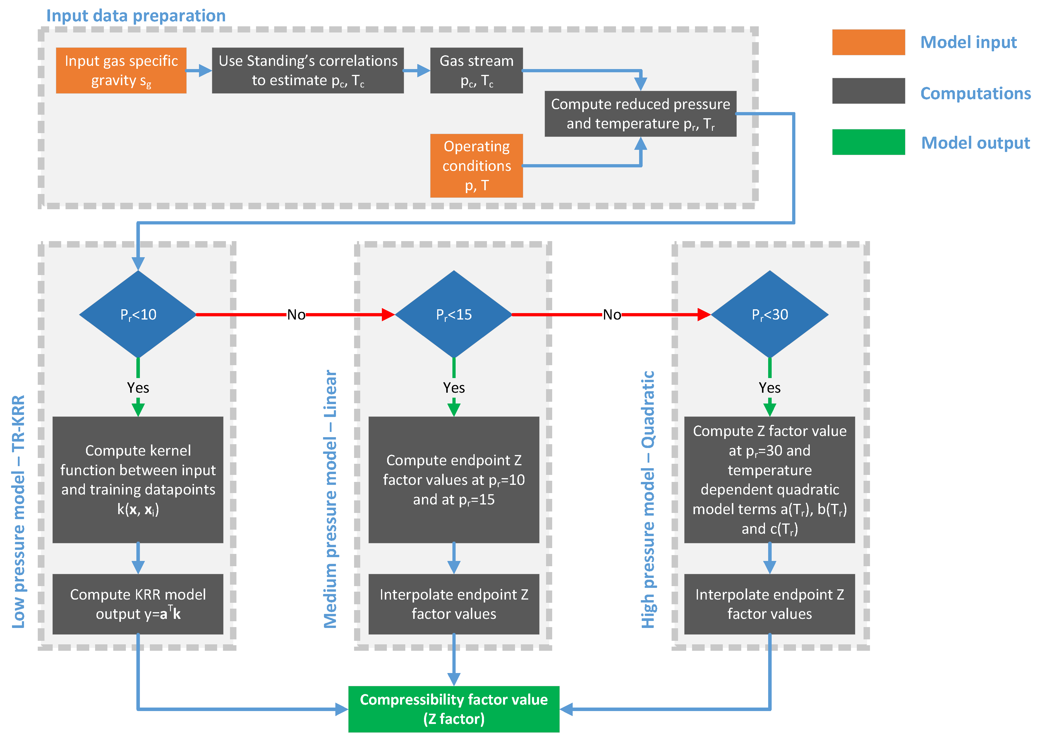
The objective of this study is to develop a numerical model to predict the Z-factor of hydrocarbon gases by fitting the Standing–Katz chart so as to overcome the weaknesses of the existing methods. For this task, the reduced pressure range is split into three regions, each described with its own submodel. For low reduced pressures, a Kernel Ridge Regression (KRR) model is used, whereas a linear and a quadratic one are developed for medium and high pressures. Figure 2 provides a general sketch of the problem.
The combined model acts as a rapid and inexpensive method to estimate the compressibility factor of a gas stream accurately. Compared to most existing methods, it can be safely used to provide Z-factor values in an extended operating range of reduced pressure values up to p r = 30 , which fully covers all upstream operations and most of the downstream ones. Unlike other numerical models, it takes advantage of the simplicity of the industry standard Standing–Katz diagram, thus ensuring a simple form and guaranteeing continuity of the Z-factor value and its derivative, hence smooth and physically-sound values. Additionally, the developed model can be utilized for the direct calculation of the Z-factor of any hydrocarbons mixture, even in the presence of impurities such as N 2 , CO 2 , and H 2 S. The model’s accuracy combined with the guaranteed continuity of the compressibility factor derivatives with respect to pressure and temperature renders it as the perfect tool to predict gas density in all petroleum engineering applications. Such applications include, but are not limited to, oil and gas reserves’ estimation and reservoir modeling, as well as fluid flow in the wellbore, the pipeline system, and the surface processing equipment.
Nevertheless, it should be pointed out that the proposed method has been designed to reproduce the Standing–Katz chart; hence, it can only be used for hydrocarbon mixtures such as those against which the standard diagram has been developed. Therefore, it might not be applicable to mixtures encountered in chemical plants, especially those comprised of non-hydrocarbon and/or polar compounds. Additionally, the non-rigorous background of the method does not allow for safe extrapolation of the operating conditions beyond those of the original chart, unlike a rigorous, although computationally-demanding, tuned multi-parameter equation of state model.
The rest of the paper is organized as follows: In Section 2, the proposed methodology is described in detail, including discussions on the data generation, the Truncated Regularized Kernel Ridge Regression (TR-KRR) method, and the numerical approach followed. The method’s performance and related computational issues are discussed in Section 3. Three example applications demonstrating the efficiency of the proposed method are presented in Section 4. The conclusions are stated in Section 5.

2. Methodology

Thorough examination of the standard Standing–Katz chart and its extension to high reduced pressures (Figure 3) indicates that it can be split into two regions along the reduced pressure axis based on the complexity of the isotherms shape. Indeed, at p r values below 10, the change of the Z-factor versus reduced pressure exhibits complex behavior with specific minima and varying curvature at most of the isotherms, thus indicating proximity to critical fluid behavior. On the other hand, for p r 10 , the isotherms exhibit a perfectly straight line shape up to the maximum p r value of 15. By further examining the supplementary Z-factor chart [12], it is clear that the Z-factor also varies linearly with reduced pressure. Moreover, the average slope at each isotherm in the p r [ 15 , 30 ] range exhibits a very slight change (of less than 0.5%) compared to the slope in the [ 10 , 15 ] range. As a result, three distinct regions can be identified in the S-K chart, and each one of them needs to be treated separately by its own modeling technique. This way, the use of “blind”, data-driven machine learning methods can be limited to the complex behavior of the low pressure region, whereas simpler models directly adopting the inherent linearity of the Z-factor with respect to p r can be generated for p r values above 10. For the sake of notation simplicity, the low, medium, and high pressure range will be labeled by L = [ 0 , 10 ] , M = [ 10 , 15 ] , H = [ 15 , 30 ] respectively.

2.1. The Low Pressure Range

In this work, the utilization of the Kernel Ridge Regression method (KRR), to be discussed in detail in Appendix A, is proposed as the appropriate machine learning tool to deal with the prediction of the Z-factor at low reduced pressures. This method aims at generating a model y ^ = f ( x ) that relates optimally a set of N recorded input and output pairs, x i and y i , i [ 1 , N ] , respectively, usually observed through an experimental process. In the present case, the input and output correspond to x = [ T r , p r ] , x R 2 and y = Z ( T r , p r ) , and they are obtained by digitizing the S-K chart. Therefore, for the low pressure range, the Z-factor is given by an expression of the form:
y ^ = α T k ( x )
where:
k = k ( x , x 1 ) , , k ( x , x N ) T
and vector k contains kernel functions k ( x , x i ) that involve the conditions x at which the Z-factor needs to be computed, as well as the pressure and temperature conditions of the training points x i . The common choices for the kernel function k ( x , y ) are the polynomial one k ( x , y ) = ( x T y + 1 ) c with c N * as the polynomial degree and the Radial Basis Function (RBF) kernel k ( x , y ) = exp ( 1 / σ | | x y | | 2 ) where σ > 0 is the width of the kernel [34].
The coefficients vector α is computed as a function of the training data x i and y i , so as to minimize the deviation between the model estimates on all training data points y ^ = K α and the digitized Z-factor values of all training data points y . The kernel matrix is defined by K = { k i j } = { k ( x i x j ) } , where x i and x j correspond to the inputs of any pair of data points. To satisfy the deviation minimization requirement, α is given by:
α = ( K + λ I N ) 1 y
where λ corresponds to a positive regularization parameter value that is introduced to avoid overfitting [35] and I N is the identity matrix of size N x N .
Although α is obtained from the solution of a linear system, the fact that matrix K + λ I N can be very large and dense renders the solution for α in Equation (7) as a very slow process with time complexity of O ( n 3 ) [35]. To treat that issue, one should revert to iterative linear systems solving methods such as the Conjugate Gradient (CG), and placing a threshold on the number of iterations leads to what is called the truncated Newton. Maalouf and Homouz [35] combined KRR with the truncated Newton method and developed a TR-KRR algorithm that is very fast to train. Interested readers should refer to Maalouf and Homouz [35] for a detailed description of TR-KRR.
The data used for the development of the proposed low reduced pressure TR-KRR model have been obtained by digitizing the original Standing–Katz chart for natural hydrocarbon gases and its extension at higher pressures [12]. Firstly, the isotherms of the standard chart, that is T r [ 1.05 , 1.45 ] in steps of 0.05, T r [ 1.5 , 2.0 ] in steps of 0.1, and T r [ 2.2 , 3.0 ] in steps of 0.2, were digitized for the full pressure range of p r [ 0.1 , 10.5 ] in steps of 0.1, thus leading to a total of 105 points per isotherm.
Subsequently, the dataset was densified by computing the estimated Z-factor values for the missing isotherms, so as to get a fixed T r density of 0.05. As such isotherms are not plotted on the S-K chart, they were inferred by invoking the H-Y method. More specifically, to estimate Z S K T r ( p r ) at some reduced temperature T r and reduced pressure p r , the digitized values at the neighboring isotherms and at p r need first to be picked from the chart, i.e., Z S K T r ( p r ) and Z S K T r + ( p r ) , where subscript S K denotes the S-K chart and superscripts T r and T r + denote the closest neighboring isotherms. As an example, consider the case of T r = 1.75 (which is not shown in the original S-K chart) for which T r = 1.7 and T r + = 1.8 . Subsequently, the corresponding Z-factor values at all three reduced temperatures T r , T r , and T r + and at p r are also computed by means of the H-Y method to obtain Z H Y T r ( p r ) , Z H Y T r ( p r ) and Z H Y T r + ( p r ) . Finally, the Standing–Katz Z-factor estimate Z ^ S K T r at T r is computed by aligning the digitized values to the computed H-Y ones:
Z ^ S K T r = Z S K T r + ( Z S K T r + Z S K T r ) Z H Y T r Z H Y T r Z H Y T r + Z H Y T r
This way, the neighboring digitized values of the SK chart at T r and at T r + are fully adopted and further combined to the curve shape provided by the H-Y method.
To ensure smooth behavior of the KRR model at values close to the pressure and temperature range boundary, additional densification was run by introducing isotherms at T r [ 1.06 , 1.09 ] and at T r [ 2.96 , 2.99 ] , both in steps of 0.01. Similarly, the pressure range was densified at p r [ 0.012 , 0.018 ] and at p r [ 10.42 , 10.48 ] in steps of 0.002. Eventually, the total number of data points of the form { p r , T r , Z } collected by this procedure was 5616.

2.2. The Medium Pressure Range

For reduced pressure values in 10 p r 15 , a linear model is proposed that interpolates temperature-dependent endpoint Z-factor values at p r = 10 and at p r = 15 with pressure in the following form:
Z M ( p r , T r ) = Z ( T r ) | p r = 10 + Z ( T r ) | p r = 15 Z ( T r ) | p r = 10 p r 10 5
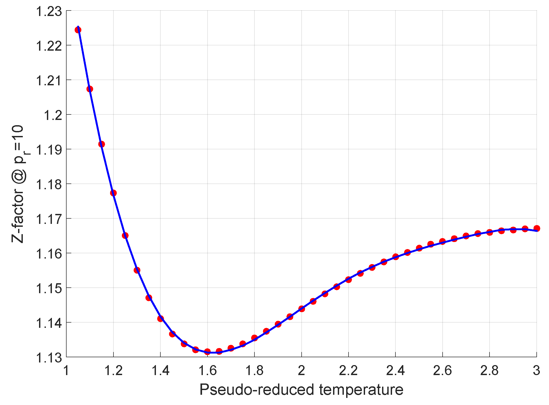
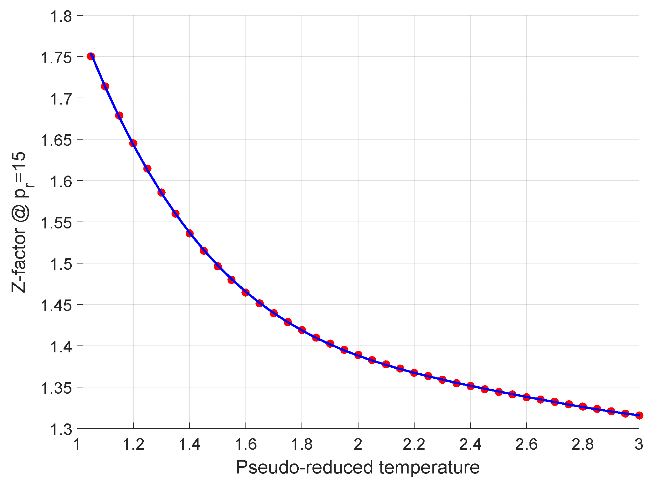
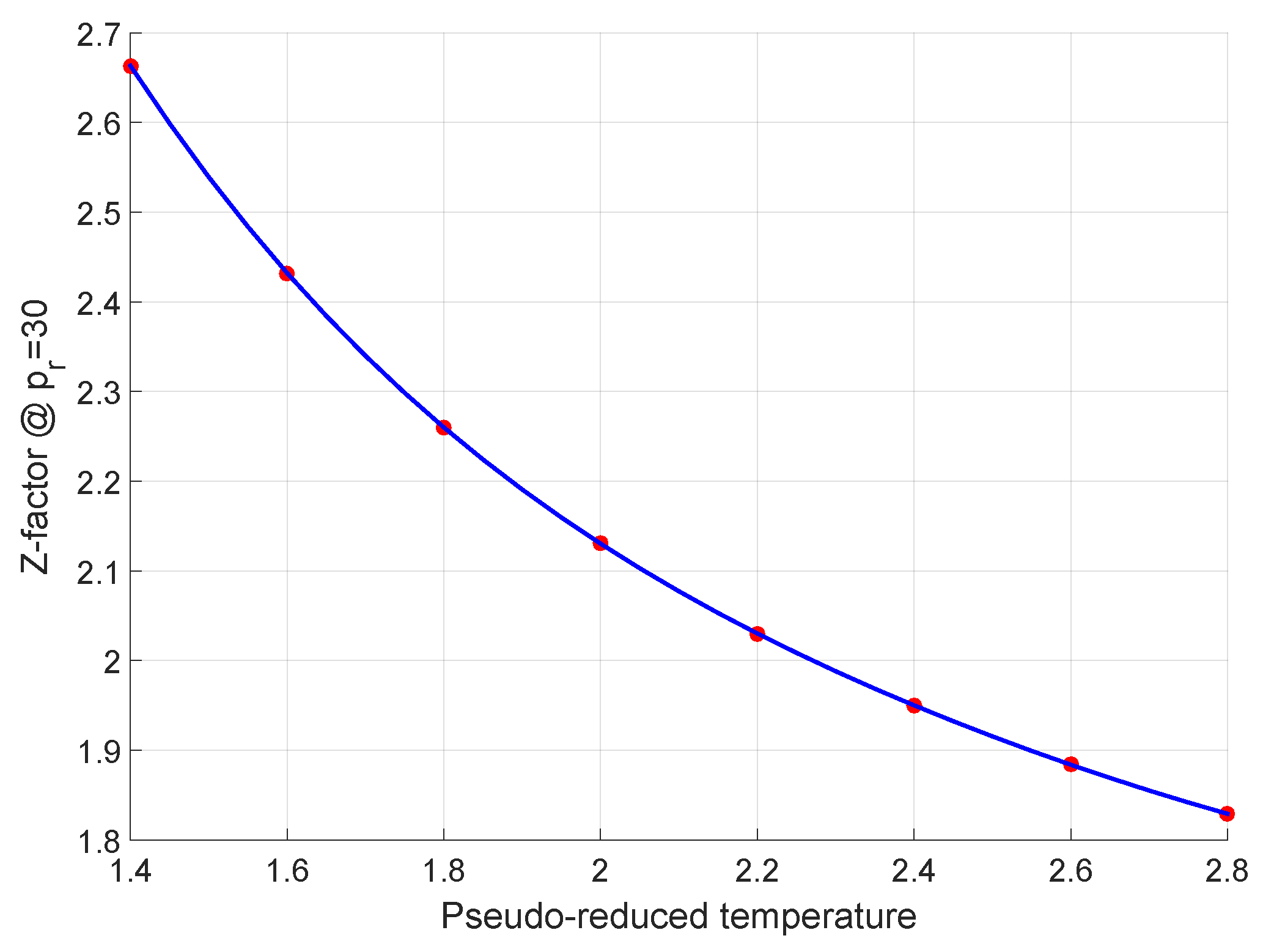
The endpoint Z-factor values at p r = 10 and at p r = 15 have been acquired from the S-K chart and further interpolated with temperature by means of polynomials of T r , which are given in Appendix B. The plot of the digitized points and their interpolants for Z ( T r ) | p r = 10 and Z ( T r ) | p r = 15 are shown in Figure 4 and Figure 5, respectively.

2.3. The High Pressure Range

Although the Z-factor values in the high pressure range 15 p r 30 exhibit a straight line shape (as was the case with p r [ 10 , 15 ] ), we propose the use of a quadratic model of reduced pressure to interpolate the temperature-dependent endpoint Z-factor values at p r = 15 and at p r = 30 with pressure. This additional degree of freedom allows the interpolating model not only to satisfy the endpoint values, but also to ensure continuity of the Z-factor derivative value at p r = 15 . This way, the continuity of the gas compressibility when switching from the medium pressure model Z M ( p r , T r ) to the high pressure one Z H ( p r , T r ) is guaranteed. Based on those requirements, the high pressure model is defined by:
Z H ( p r , T r ) = a ( T r ) p r 2 + b ( T r ) p r + c ( T r )
where the temperature-dependent terms are given in Appendix C. The plot of Z ( T r ) | p r = 30 is shown in Figure 6.

2.4. The Combined Model

To further ensure the value and derivative continuity between Z L ( p r , T r ) and Z M ( p r , T r ) , we recommend a weighted average scheme that switches mildly between the two models in the p r [ 10 , 10.5 ] region by using:
Z ( 10 10.5 ) ( p r , T r ) = w Z L ( p r , T r ) + ( 1 w ) Z M ( p r , T r )
where:
w = 1 p r 10 0.5
Therefore, the combined Z-factor prediction algorithm is given by the following scheme:
Z ( p r , T r ) = Z L ( p r , T r ) , 0 p r 10 , 1 . 05 T r 3 . 0 , w Z L ( p r , T r ) + ( 1 w ) Z M ( p r , T r ) , 10 p r 10 . 5 , 1 . 05 T r 3 . 0 , Z M ( p r , T r ) , 10 . 5 p r 15 , 1 . 05 T r 3 . 0 , Z H ( p r , T r ) , 15 p r 30 , 1 . 4 T r 2 . 8 .
It is straightforward to show that derivative continuity at p r = 15 is guaranteed, that is:
p r Z M ( p r , T r ) | p r = 15 = Z ( T r ) | p r = 15 Z ( T r ) | p r = 10 15 10 = p r Z H ( p r , T r ) | p r = 15

3. Results and Discussion

To obtain a reliable KRR model for the prediction of the Z-factor at p r 10 parameters σ , λ , and N, corresponding to the RBF kernel width, the strength of the penalty term and the number of training data points, respectively, need to be determined. For that task, the ten-fold cross-validation technique was used to ensure generalization [36]. In the n-fold cross-validation and for each combination of possible parameters values, the data were split into n-folds, and ( n 1 ) folds were used for training, while the remaining fold was reserved for testing. This process was iterative until all folds were tested. Finally, the optimal model was selected so as to exhibit balanced error and minimum absolute relative error against the training and the validation datasets, as well as nearly equal training and prediction error. The examined range of the parameters was σ [ 0.001 , 0.1 ] , λ [ 0.0001 , 0.1 ] and N { 1000 , 2000 , 3000 , 4000 } . After repeatedly examining all possible combinations, it was found that optimal performance was obtained by selecting σ = 0.01 , λ = 0.001 and N = 3000 . Clearly, model accuracy is expected to be further improved when increasing the number of training data points. However, the selected population size is the minimum that led to a ratio of the training and validation errors very close to unity, thus minimizing the risk of overfitting.
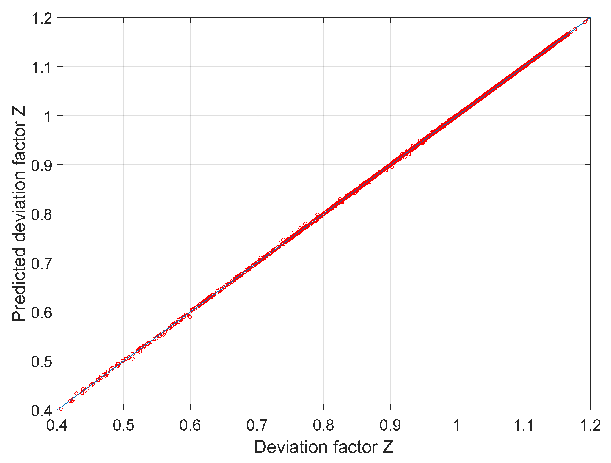
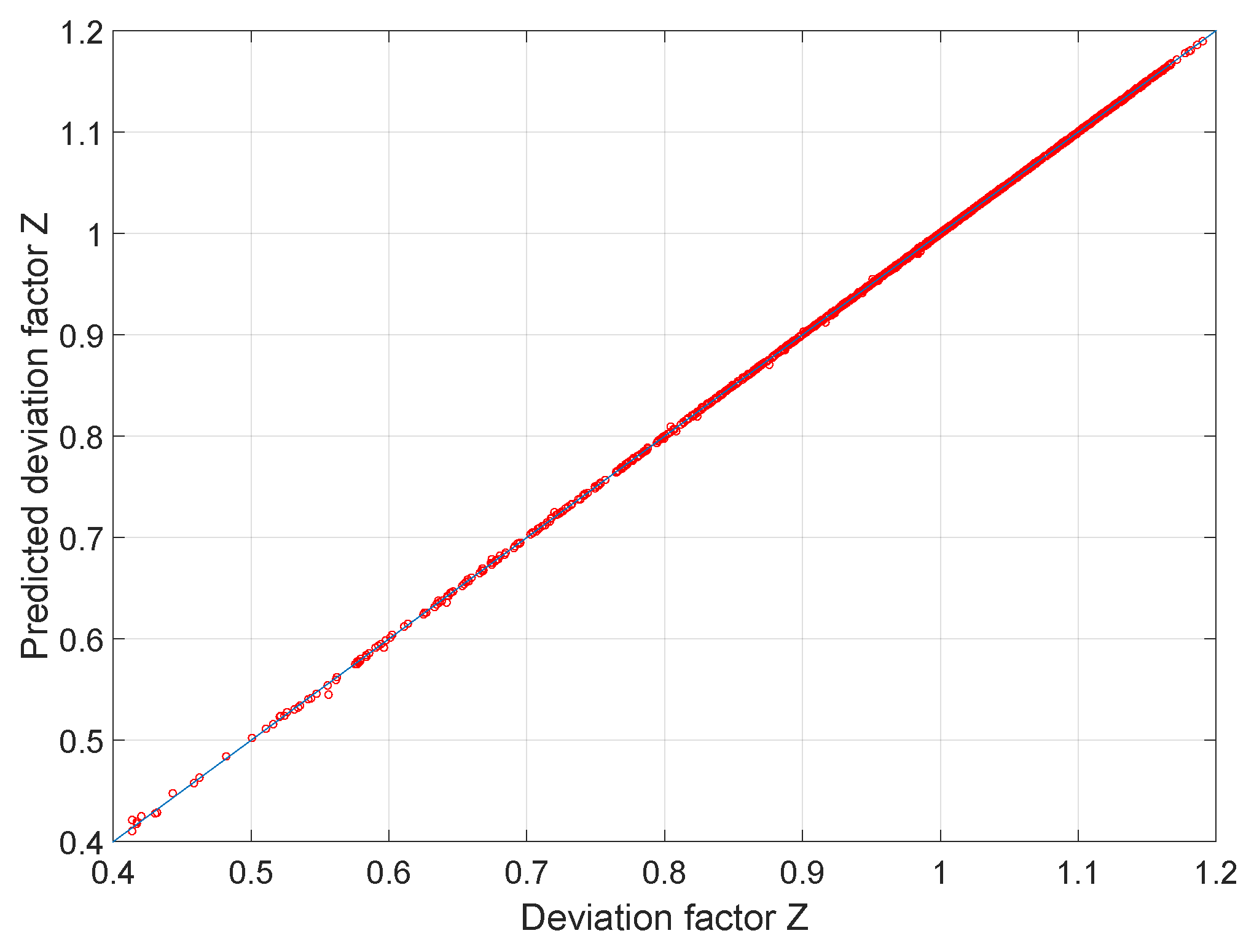
The performance of the optimal TR-KRR model is shown in Table 1. Judging from the mean errors, the model was perfectly justified, exhibiting no bias. Moreover, it exhibited excellent agreement with the S-K chart as the mean absolute relative error was only 0.04% for both the training and the validation dataset, and the worst case error that might be observed was less than 2%, which is significantly better than all conventional methods. The scatter plots of the model performance for the training and prediction dataset are shown in Figure 7 and Figure 8, respectively. A plot of the Z-factor surface that has been produced by interpolating the training data points together with the validation data points is shown in Figure 9.
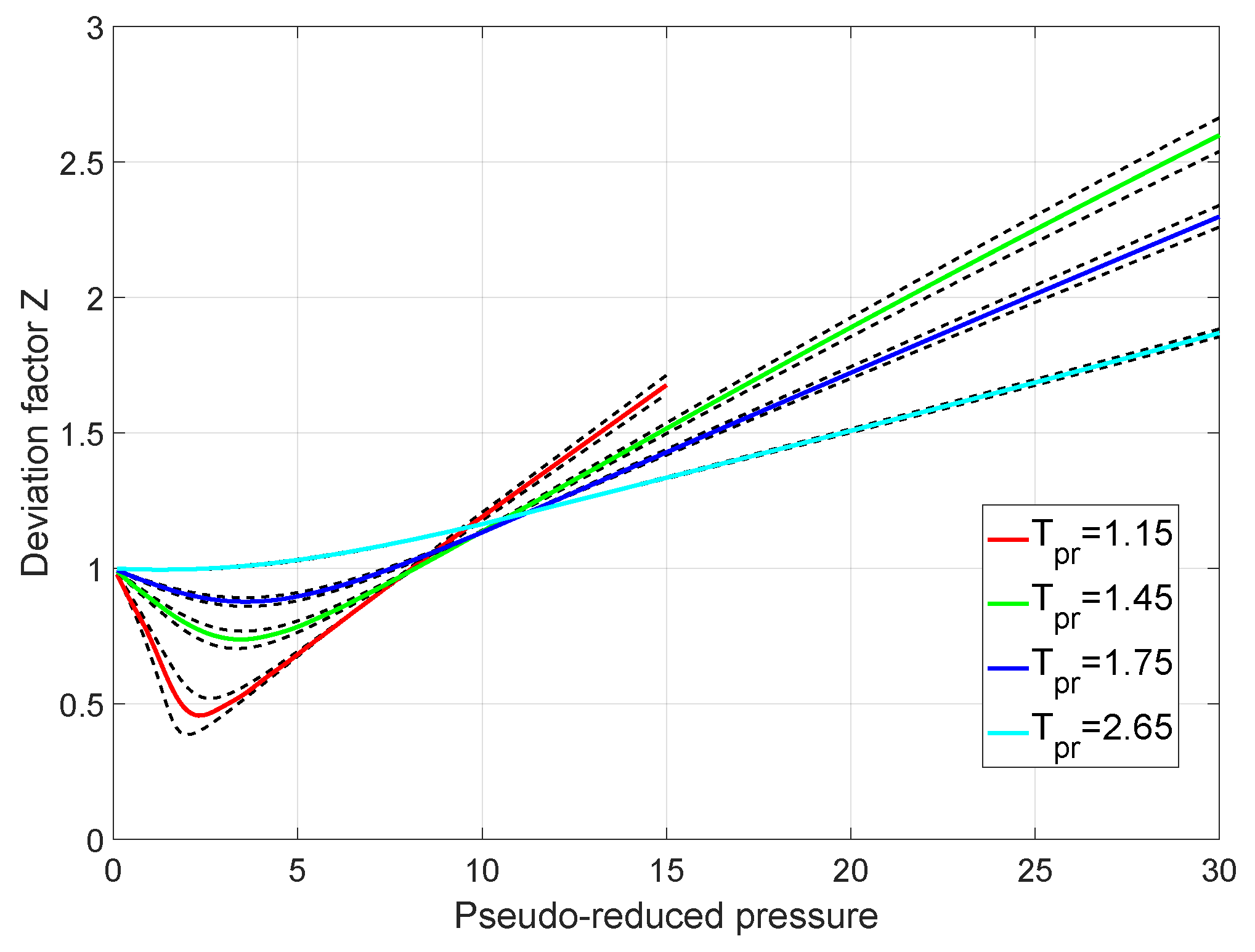
In terms of computational time required for training, TR-KRR was very efficient, and this agrees with the findings of Maalouf and Homouz [35] that the biggest strength of TR-KRR method lies in its superior efficiency over other state-of-the-art methods, such as SVM [32]. In addition to predicting accurately the original temperature curves contained in the dataset, TR-KRR was capable of predicting new temperature curves. Figure 10 provides four examples of two additional temperature curves predicted by KRR at T r = 1.15 , T r = 1.45 , T r = 1.75 and at T r = 2.65 . In all cases, the predicted curves fell smoothly between neighboring Standing–Katz curves.
Implementing the TR-KRR prediction of the Z-factor for low p r and any given T r can be done conveniently according to the following simple formula:
Z = i N α i d i ( p r , T r )
where
d i = exp 1 σ ( T ¯ r i T ¯ r ) 2 + ( p ¯ r i p ¯ r ) 2
p r i , T r i are the training population pseudo-critical temperature and pressure data, respectively, and the bar character denotes normalized inputs given by:
p ¯ r = p r min ( p r i ) max ( p r i ) min ( p r i ) 1 2 and T ¯ r = T r min ( T r i ) max ( T r i ) min ( T r i ) 1 2
The derivative of the Z-factor with respect to pressure, needed to calculate the fluid’s isothermal compressibility by means of Equation (4), is given by:
θ Z θ p = i = 1 N θ Z θ d i θ d i θ p ¯ r θ p ¯ r θ p r θ p r θ p = 2 σ p c max ( p r i ) min ( p r i ) i = 1 N α i d i ( p ¯ r i p ¯ r )

4. Case Studies

Three case studies are presented to further demonstrate the efficiency of the derived model.

4.1. Case Study 1

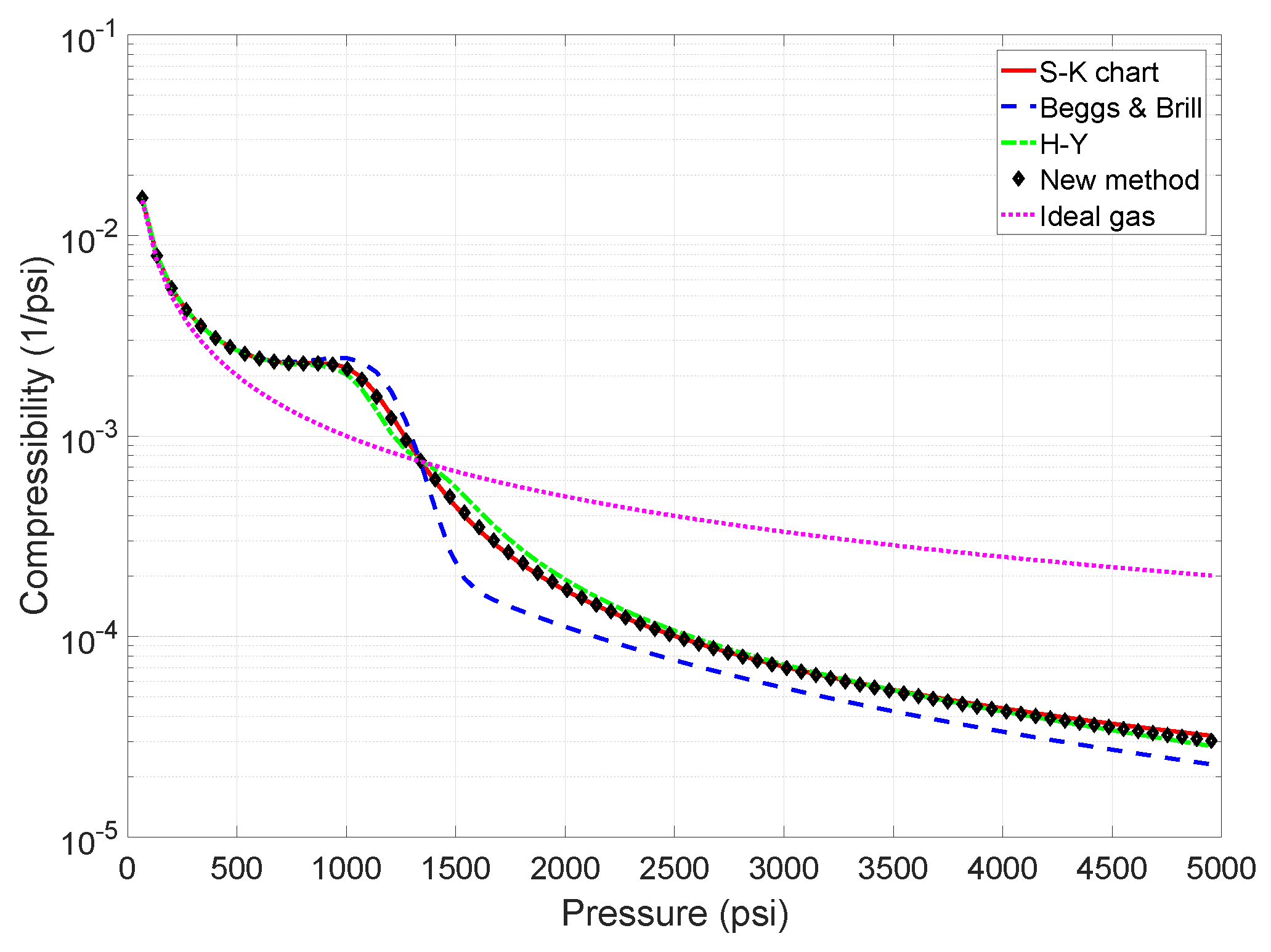
In this case study, we considered the effect of the Z-factor accuracy to that of the gas compressibility, which is a derived property according to Equation (4). The composition of the gas mixture studied was z C 1 = 82 % , z C 2 = 10 % , z C 3 = 5 % , z C 4 = 3 % , and its critical pressure and temperature were estimated at 670 psi and 215 F, respectively, by means of Standing’s gas specific gravity-based correlations. The isothermal compressibility of the gas mixture has been computed at a temperature of 236 F and for a pressure range from nearly atmospheric to 5000 psi. The methods utilized were the most commonly-used ones, that is the iterative algorithm of Hall and Yarborough, the correlation of Beggs and Brill, and the one proposed in this work. Note that the test temperature has been deliberately selected so as to demonstrate the performance of the examined methods at near critical conditions.
The performance of all methods and their comparison against the exact S-K chart is shown in Figure 11.
The compressibility of the ideal gas (i.e., c = p 1 ), obtained by totally neglecting the deviating effect of the Z-factor, is also shown. Judging from the difference between the ideal gas compressibility and that obtained by any other method, it can be readily seen that the effect of the Z-factor on the gas compressibility was quite significant. Indeed, at high pressures close to 5000 psi, introducing the Z-factor effect reduced the compressibility by almost one order of magnitude, thus verifying the need for accurate Z-factor determination algorithms.
As expected, at very low pressures, where the gas behaves almost ideally, the effect of the Z-factor was minimal; hence, all methods ended up with very close isothermal compressibility estimates. However, this was not the case at higher pressures where the Beggs and Brill correlation performed quite poorly and the computed compressibility exhibited deviations as high as 47% at the near critical region. For example, at 1500 psi, the compressibility value obtained by the original S-K chart was 4.3 × 10 4 psi 1 , whereas the Beggs and Brill one was only 2.3 × 10 4 psi 1 . On the other hand, the H-Y method, despite its convergence issues, performed better by predicting 5.4 × 10 4 psi 1 , leading to an error of 25%. The method proposed in this work was significantly more accurate, as it led to a value of 4.5 × 10 4 psi 1 , which corresponds to a relative error of only 5%.
A similar situation was observed at high pressures where the S-K value was 3.1 × 10 5 psi 1 . The values obtained by Beggs and Brill, Hall and Yarborough, and the new method were 2.3 × 10 5 psi 1 , 2.8 × 10 5 psi 1 and 3.0 × 10 5 psi 1 , leading to relative errors of 25%, 10%, and 3%, respectively, thus demonstrating the superiority of the new method.

4.2. Case Study 2

We now consider the dependency of the pressure drop of a gas stream flowing in a pipeline on the accuracy of the utilized Z-factor values. The gas was assumed to be a dry one, the exact composition of which was z C H 4 = 0.78 , z C 2 H 6 = 0.04 , z C 3 H 8 = 0.02 , z C 4 H 10 = 0.01 , z C O 2 = 0.15 with a molar mass value of 21.74 g/mole and γ g = 0.7504. The gas was assumed to be compressed at an initial pressure of 1200 psi and introduced to a 30 mile-long pipeline of internal diameter of 6” at ambient temperature (60 F) and at a flow rate of 30 MMscf/d. The flow was assumed to be isothermal, and the heating effect of gas compression was ignored. Moreover, to simplify calculations, it was also assumed that the pipeline network exhibited no elevation changes. The outlet pressure for a given pipeline length can be estimated by:
p o u t = p i n 2 s g f Z T L D 5 q S C 77.54 p b T b 2
where f is the friction factor, p i n and p o u t is the inlet and outlet pressure (psi), T is the pipeline temperature (R), L is the pipeline length (miles), D is the diameter (in), p b , T b are the standard conditions (psi and R, respectively), and q S C is the flow rate reported at standard conditions (scf/d).
From the expression above, it is clear that the outlet pressure for given pipeline geometry and gas pump efficiency was directly related to the Z-factor. Therefore, various outlet pressures will be obtained depending on the method utilized to estimate the deviation factor. In this example, the methods of Hall and Yarborough, Beggs and Brill, the proposed method in this work, and the direct use of the Standing–Katz chart were utilized. The pseudo-critical properties were computed as functions of gas s g using Standing’s recommended expressions, thus leading to p p c = 667.1 psi and T p c = 404.9 R. Correspondingly, the reduced conditions in this test case were equal to p p r = 1.8 and T p r = 1.283 . The resulting computed outlet pressures are shown in Table 2.
It can be readily seen that although the prevailing conditions were well within the valid range of the tried methods, the Beggs and Brill correlation exhibited significant deviation from the original S-K chart, which, eventually, led to a significant difference of 4 bar, whereas the H-Y methods performed better, but still exhibited an error of 2.5 bar. On the other hand, the proposed approach provided an accurate estimate of the Z-factor, which, in turn, led to an outlet pressure deviation of 10 psi, i.e., less than 1 bar.

4.3. Case Study 3

The interpretation of production data from a gas reservoir so as to estimate the reservoir reserves by means of the gas material balance method is demonstrated in this case study. When applied to a dry gas reservoir between production start and current time, the material balance equation states that:
p Z ( p ) = p i Z ( p i ) p i Z ( p i ) G p G
where p and G p refer to the pressure and recorded cumulative gas production at the current time instance, while p i denotes the initial reservoir pressure, and G corresponds to the reserves. Evidently, by recording a single pressure drop and the observed gas production, the equation can be directly solved for G. However, as such measurements (especially the pressure one) are prone to errors, most engineers prefer to keep recording p and G p for a longer period and then compute the statistically-optimal G value in the least squares sense. By rewriting the above equation in the following form:
p Z ( p ) = p i Z ( p i ) 1 G p i Z ( p i ) G p
it becomes clear that the observed p / Z ratio at any pressure is a linear function of the cumulative production G p . Therefore, by fitting the p / Z ratios with a linear function of the form p / Z = a G p + b and considering that G p = G when p = 0 , i.e., that the reserves will be fully produced only when the reservoir pressure becomes equal to zero, we obtain:
p Z = a + b G p G = lim p 0 G p = a b
In this example, the pressure and production data, shown in Table 3, from a large gas field have been utilized. The fluid composition and properties were the same to those in Case study 1 and so were the computational methods used to estimate the p / Z ratios. The estimated gas reserves G as obtained by each method are shown in Table 4.
As expected, the results exhibited significant differences depending on the method utilized. Once again, the Beggs and Brill method exhibited worst performance, leading to a missed gas volume of 4.36 billion scf of gas, whereas the Hall and Yarborough method performed better by limiting the missed reserves to 1.05 Bscf. On the other hand, the method proposed in this work underestimated reserves only by 0.61 Bscf, which is the most accurate estimate compared to all other approaches. It should be noted that, unlike density calculations, when it comes to estimating hydrocarbon reserves, the exact value of the Z-factor did not really affect the results. To show that, we rewrite Equation (20) by replacing the Z-factor with a random multiple of that, that is:
p a Z ( p ) = p i a Z ( p i ) p i a Z ( p i ) G p G
The reserves estimate from a single measurement ( p , G p ) is given by:
G = p i / ( a Z ( p i ) ) p i / ( a Z ( p i ) ) p / ( a Z ( p ) ) G p
where, clearly, parameter a cancels, thus showing that any multiple of the Z-factor will lead to the same reserves estimate. As was the case with the prediction of gas compressibility, this result demonstrates the need for the Z-factor prediction models to preserve the shape of the original S-K curves, thus exhibiting physically-sound derivatives and isothermal compressibility values.

5. Conclusions

In this work, a new, efficient, consistent, and physically-sound method is presented for the prediction of the Z-factor of natural gas streams. Our conclusions are summarized as follows:
  • At low reduced pressures where critical behavior might be observed and dependency on pressure is quite complex, the proposed method utilized the non-linear regression TR-KRR modeling technique to predict the gas compressibility factor.
  • Our results indicated that despite the abruptly changing slope of the Z-factor isotherms, the TR-KRR model was highly accurate and efficient at predicting Z-factor.
  • The simplicity of the original S-K chart and its extension at medium and high pressures was directly inherited by the corresponding linear and quadratic submodels developed for the prediction of the Z-factor.
  • Special attention has been paid to ensure a natural model derivative behavior, so as to end up with reliable isothermal compressibility values.

Author Contributions

Conceptualization, M.M. and N.K.; methodology, M.M. and D.H.; software, V.G.; validation, V.G. and D.H.; formal analysis, V.G., D.H., M.M., and K.P.; investigation, K.P., M.M., V.G., N.K., and D.H.; resources, K.P., M.M., D.H., and V.G.; data curation, V.G., M.M., and D.H.; writing, original draft preparation, M.M., K.P., and V.G.; visualization, V.G. and D.H.; funding acquisition, K.P.

Funding

This publication is based on work supported by the Khalifa University of Science and Technology under Award No. RC2-2018-024.

Acknowledgments

The authors would like to acknowledge the support by Khalifa University of Science and Technology under Award No. RC2-2018-024.

Conflicts of Interest

The authors declare no conflict of interest.

Appendix A. Details of the Z L Model

Regression [37] aims at generating a model y = f ( x ) that relates optimally a set of N recorded input-output pairs x i and y i , i [ 1 , N ] , respectively, usually observed through an experimental process. The input vector may contain d 1 features, also known as parameters or attributes, whereas, for convenience, unity is further added to the input vector, so that x R d . Linear regression assumes a vector β such that:
y = f ( x ) = x T β + ϵ = y ^ + ϵ
By collecting all inputs in matrix X R N × d and all outputs (responses) in y R N , linear regression for the full dataset generalizes to:
y = f ( X ) = X β + ϵ = y ^ + ϵ
The weights vector β needs to be optimized so that error ϵ exhibits its minimum value over all available training pairs, and the optimization problem is defined by:
β = argmin J ( β )
where the total error to be minimized is given by:
J ( β ) = 1 2 i = 1 i = N ϵ i 2 = ϵ T ϵ = 1 2 ( y y ^ ) T ( y y ^ ) = 1 2 ( y X β ) T ( y X β )
The closed-form solution of this optimization problem, that is β for which β J = 0 , is given by the Moore–Penrose inverse [38] of the data matrix X , that is:
β = ( X T X ) 1 X T y
Regularization [39] needs to be used to avoid poor estimation of the regression coefficients due to the instability of the solution of Equation (A5). This idea lies in “penalizing” high coefficients values, which, essentially, improves the rank of the covariance matrix X T X . Therefore, ridge regression aims at minimizing the modified objective function:
J ( β ) = 1 2 ϵ T ϵ = 1 2 ( y X β ) T ( y X β ) + λ 2 β T β
which is optimized at:
β = ( X T X + λ I d ) 1 X T y
where I d is a d × d identity matrix and λ is a positive constant that adjusts the penalty term.
In order to extend to non-linear relationships, the dual form [40] needs firstly to be introduced. Let β be expressed as a linear combination of the data points, i.e.,
β = X T α
By replacing back in the regression model, we obtain:
y = X X T α + ϵ = G α + ϵ
where the Gramian matrix G = XX T . This way, the objective function to be minimized is now expressed in terms of the new coefficients vector α and turns into:
f ( α ) = 1 2 ( y G α ) T ( y G α ) + λ 2 α T α
and it is optimized at:
α = ( G + λ I N ) 1 y
In this case, the benefit of the dual form is that solution α depends on G , that is only on dot products of the input vectors x i . The price to be paid is that the size of α is equal to the number of data points N, whereas the size of β is equal to the number of features d.
Kernel Ridge Regression (KRR) [34] can be thought of as an extension of the linear regression dual form, so as to handle non-linear relationships between the input and output. This is done simply by including a nonlinear map, ϕ ( . ) , which projects the original input data x into a high-dimensional, even infinite-dimensional, feature space F such that:
ϕ : x R d ϕ ( x ) F .
thus leading to the generalized Gramian G = Φ ( X ) Φ ( X ) T and the regression model:
y = Φ ( X ) Φ ( X ) T α + ϵ = G α + ϵ
This way output, y is non-linear in the input x , but it is still linear in the coefficients α . In general, the non-linear mapping ϕ ( . ) is unknown; however, the solution is based mainly on linear dot products of the images ϕ ( x ) . To overcome the difficulty in working with dot products of high dimensionality in the feature space F , kernel functions are utilized, which compute a dot product in F as a function of the dot product of the original inputs, that is ϕ ( x ) T ϕ ( y ) = k ( x T y ) for some suitable scalar function k ( . ) . The most commonly-used kernels are the polynomial kernel k ( x , y ) = ( x T y + 1 ) c with c N * as the polynomial degree and the Radial Basis Function (RBF) kernel k ( x , y ) = exp ( 1 / σ | | x y | | 2 ) where σ > 0 is the width of the kernel [34]. Based on that, the Kernel Ridge Regression model (KRR) [35] is given by:
y = K α + ϵ
where K = { k i j } = { k ( x i x j ) } , and the coefficients vector α is computed by minimizing:
f ( α ) = 1 2 ( y K α ) T ( y K α ) + λ 2 α T α
The solution now is given by:
α = ( K + λ I N ) 1 y
Although α is obtained from the solution of a linear system, the fact that matrix K + λ I N can be very large and dense renders the solution for α in Equation (A16) as a very slow process with time complexity of O ( n 3 ) [35]. To treat that issue, one should revert to iterative linear systems, solving methods such as the CG, and placing a threshold on the number of iterations leads to what is called the truncated Newton. Maalouf and Homouz [35] combined KRR with the truncated Newton method and developed a TR-KRR algorithm that is very fast to train. Interested readers should refer to Maalouf and Homouz [35] for a detailed description of TR-KRR.
Once the coefficients values α have been optimized, the predictive model for any new input x is given by the following simple, linear-in-the-weights model:
y = α T k ( x )
where:
k = k ( x , x 1 ) , , k ( x , x N ) T
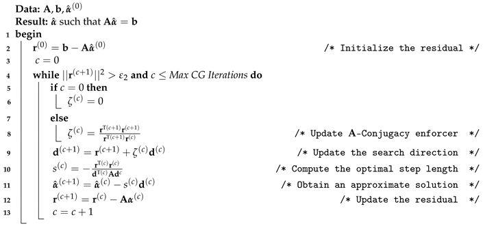
In this work, TR-KRR is terminated when the CG residual is less than a threshold ε = 0.5 or the maximum number of 200 CG iterations are reached.
Algorithm 1: Linear CG for computing α ^ . A = K + λ I N , b = y
Energies 12 02577 i001

Appendix B. Details of the Z M Model

The linear model providing the Z-factor in 10 p r 15 interpolates the endpoint Z-factor values at p r = 10 and at p r = 15 in the following form:
Z M ( p r , T r ) = Z ( T r ) | p r = 10 + Z ( T r ) | p r = 15 Z ( T r ) | p r = 10 p r 10 5
The temperature-dependent endpoint Z-factor values have been acquired from the S-K chart and further interpolated by means of polynomials of T r , and they are defined by the following expressions:
Z ( T r ) | p r = 10 = 0.024466 T r 6 + 0.284414 T r 5 1.281582 T r 4 + 2.712782 T r 3 2.407661 T r 2 + 0.079238 T r + 1.883774
and:
Z ( T r ) | p r = 15 = 0.048200 T r 4 0.502345 T r 3 + 1.977248 T r 2 3.546957 T r + 3.820608

Appendix C. Details of the Z H Model

To obtain Z-factor values in the high pressure range 15 p r 30 , the digitized endpoint Z-factor values at p r = 15 and at p r = 30 are interpolated by the following quadratic model:
Z H ( p r , T r ) = a ( T r ) p r 2 + b ( T r ) p r + c ( T r )
where:
a ( T r ) = Z ( T r ) | p r = 30 4 Z ( T r ) | p r = 15 + 3 Z ( T r ) | p r = 10 225
b ( T r ) = Z ( T r ) | p r = 15 Z ( T r ) | p r = 10 5 30 a ( T r )
c ( T r ) = Z ( T r ) | p r = 15 225 a ( T r ) 15 b ( T r ) ;
and:
Z ( T r ) | p r = 30 = 0.090371 T r 4 0.957066 T r 3 + 3.938661 T r 2 7.726749 T r + 8.039752
From Equation (A23), it can be seen that the denominator is very large compared to the nominator, thus verifying that the introduced curvature due to parameter a is very small and that Z H ( p r , T r ) is very close to a straight line.

References

  1. Tan, S.P.; Qiu, X.; Dejam, M.; Adidharma, H. Critical point of fluid confined in nanopores: Experimental detection and measurement. J. Phys. Chem. C 2019, 123, 9824–9830. [Google Scholar] [CrossRef]
  2. Qiu, X.; Tan, S.P.; Dejam, M.; Adidharma, H. Simple and accurate isochoric differential scanning calorimetry measurements: Phase transitions for pure fluids and mixtures in nanopores. Phys. Chem. Chem. Phys. 2019, 21, 224–231. [Google Scholar] [CrossRef] [PubMed]
  3. Qiu, X.; Tan, S.P.; Dejam, M.; Adidharma, H. Novel isochoric measurement of the onset of vapor-liquid phase transition using differential scanning calorimetry. Phys. Chem. Chem. Phys. 2018, 20, 26241–26248. [Google Scholar] [CrossRef] [PubMed]
  4. Nikpoor, M.H.; Dejam, M.; Chen, Z.; Clarke, M. Chemical-gravity-thermal diffusion equilibrium in two-phase non-isothermal petroleum reservoirs. Energy Fuels 2016, 30, 2021–2034. [Google Scholar] [CrossRef]
  5. Standing, M. Volumetric and Phase Behavior of Oil Field Hydrocarbon Systems: PVT for Engineers; California Research Corporation: Vancouver, BC, Canada, 1951. [Google Scholar]
  6. Amyx, J.W.; Bass, D.M.; Whiting, R.L. Petroleum Reservoir Engineering: Physical Properties; McGraw-Hill: New York, NY, USA, 1960. [Google Scholar]
  7. Redlich, O.; Kwong, J.N. On the thermodynamics of solutions. v. an equation of state. Fugacities of gaseous solutions. Chem. Rev. 1949, 44, 233–244. [Google Scholar] [CrossRef] [PubMed]
  8. Whitson, C.; Brule, M. Phase Behavior; SPE: Richardson, TX, USA, 2000. [Google Scholar]
  9. Reid, R.C.; Prausnitz, J.M.; Poling, B.E. The Properties of Gases and Liquids, 4th ed.; McGraw-Hill: New York, NY, USA, 1987. [Google Scholar]
  10. Zudkevitch, D.; Joffe, J. Correlation and prediction of Vapor-Liquid Equilibrium with the Redlich-Kwong Equation of State. AIChE J. 1970, 16, 112. [Google Scholar] [CrossRef]
  11. Hayden, J.G.; O’Connell, J.P. A generalized method for predicting second virial coefficients. Ind. Eng. Chem. Proc. Des. Dev. 1975, 14, 209–216. [Google Scholar] [CrossRef]
  12. Katz, D.L.; Cornell, D.; Kobayashi, R.; Poettmann, F.H.; Vary, J.A.; Elenbaas, J.R.; Weinaug, C.F. Handbook of Natural Gas Engineering; McGraw-Hill: New York, NY, USA, 1959. [Google Scholar]
  13. Wichert, E.; Aziz, K. Compressibility Factor of Sour Natural Gases. Cdn. J. Chem. Eng. 1975, 49, 267. [Google Scholar] [CrossRef]
  14. Kay, W. Gases and vapors at high temperature and pressure-density of hydrocarbon. Ind. Eng. Chem. 1936, 28, 1014–1019. [Google Scholar] [CrossRef]
  15. Stewart, W.; Burkhardt, S.; Voo, D. Prediction of pseudo-critical parameters for mixtures. In Proceedings of the AIChE Meeting, Kansas City, MO, USA, 18 May 1959; Volume 18. [Google Scholar]
  16. Sutton, R. Compressibility factors for high-molecular-weight reservoir gases. In Proceedings of the SPE Annual Technical Conference and Exhibition, Las Vegas, NV, USA, 22–26 September 1985; Society of Petroleum Engineers: London, UK, 1985. [Google Scholar]
  17. Danesh, A. Pvt and Phase Behaviour of Petroleum Reservoir Fluids; Developments in Petroleum Science, Elsevier: Amsterdam, The Netherlands, 1998. [Google Scholar]
  18. Hall, K.R.; Yarborough, L. A New EOS for Z-factor Calculations. Oil Gas J. 1973, 71, 82–92. [Google Scholar]
  19. Dranchuk, P.; Abou-Kassem, H. Calculation of z factors for natural gases using equations of state. J. Can. Pet. Technol. 1975, 14. [Google Scholar] [CrossRef]
  20. Brill, J.P.; Beggs, H.D. Two-Phase Flow in Pipes; University of Tulsa INTERCOMP Course: The Hague, The Netherlands, 1974. [Google Scholar]
  21. Azizi, N.; Behbahani, R.; Isazadeh, M. An efficient correlation for calculating compressibility factor of natural gases. J. Nat. Gas Chem. 2010, 19, 642–645. [Google Scholar] [CrossRef]
  22. Kumar, N. Compressibility Factor for Natural and Sour Reservoir Gases by Correlations and Cubic Equations of State. Master’s Thesis, Texas Tech University, Lubbock, TX, USA, 2004. [Google Scholar]
  23. Heidaryan, E.; Moghadasi, J.; Rahimi, M. New correlations to predict natural gas viscosity and compressibility factor. Fluid Phase Equilibria 2009, 218, 1–13. [Google Scholar] [CrossRef]
  24. Kareem, L.; Iwalewa, T.; Al-Marhoun, M. New explicit correlation for the compressibility factor of natural gas: linearized z-factor isotherms. J. Petrol Explor. Prod. Technol. 2016, 6, 481–492. [Google Scholar] [CrossRef]
  25. Elsharkawy, A.M. Efficient methods for calculations of compressibility, density and viscosity of natural gases. Fluid Phase Equilibria 2004, 218, 1–13. [Google Scholar] [CrossRef]
  26. Moghadassi, A.; Parvizian, F.; Hosseini, S.; Fazlali, A. A new approach for estimation of pvt properties of pure gases based on artificial neural network model. Braz. J. Chem. Eng. 2009, 26, 199–206. [Google Scholar] [CrossRef]
  27. Irene, A.I.; Sunday, I.S.; Orodu, O.D. Forecasting Gas Compressibility Factor Using Artificial Neural Network Tool for Niger-Delta Gas Reservoir. Soc. Pet. Eng. 2016. [Google Scholar] [CrossRef] [Green Version]
  28. Kamyab, M.; Sampaio, J.H.; Qanbari, F.; Eustes, A.W. Using artificial neural networks to estimate the z-factor for natural hydrocarbon gases. J. Pet. Sci. Eng. 2010, 73, 248–257. [Google Scholar] [CrossRef]
  29. Sanjari, E.; Lay, E.N. Estimation of natural gas compressibility factors using artificial neural network approach. J. Nat. Gas Sci. Eng. 2012, 9, 220–226. [Google Scholar] [CrossRef]
  30. Fayazi, A.; Arabloo, M.; Mohammadi, A.H. Efficient estimation of natural gas compressibility factor using a rigorous method. J. Nat. Gas Sci. Eng. 2014, 16, 8–17. [Google Scholar] [CrossRef]
  31. Kamari, A.; Hemmati-Sarapardeh, A.; Mirabbasi, S.-M.; Nikookar, M.; Mohammadi, A.H. Prediction of sour gas compressibility factor using an intelligent approach. Fuel Process. Technol. 2013, 116, 209–216. [Google Scholar] [CrossRef]
  32. Cristianini, N.; Shawe-Taylor, J. An Introduction to Support Vector Machines and other Kernel-Based Learning Methods; Cambridge University Press: Cambridge, UK, 2000. [Google Scholar]
  33. Mohamadi-Baghmolaei, M.; Azin, R.; Osfouri, S.; Mohamadi-Baghmolaei, R.; Zarei, Z. Prediction of gas compressibility factor using intelligent models. Nat. Gas Ind. B 2015, 2, 283–294. [Google Scholar] [CrossRef] [Green Version]
  34. Shawe-Taylor, J.; Cristianini, N. Kernel Methods for Pattern Analysis; Cambridge University Press: Cambridge, UK, 2004. [Google Scholar]
  35. Maalouf, M.; Homouz, D. Kernel ridge regression using truncated newton method. Knowl.-Based Syst. 2014, 71, 339–344. [Google Scholar] [CrossRef]
  36. Efron, B.; Tibshirani, R.J. An Introduction to the Bootstrap; Chapman & Hall/CRC: Vancouver, BC, Canada, 1994. [Google Scholar]
  37. Rencher, A. Methods of Multivariate Analysis; Wiley Interscience: Hoboken, NJ, USA, 2002. [Google Scholar]
  38. Shores, T. Applied Linear Algebra and Matrix Analysis; Springer: Berlin/Heidelberg, Germany, 2007. [Google Scholar]
  39. Bishop, C.M. Pattern Recognition and Machine Learning; Oxford University Press: Oxford, UK, 2006. [Google Scholar]
  40. Nocedal, J.; Wright, S. Numerical Optimization; Springer: Berlin/Heidelberg, Germany, 2006. [Google Scholar]
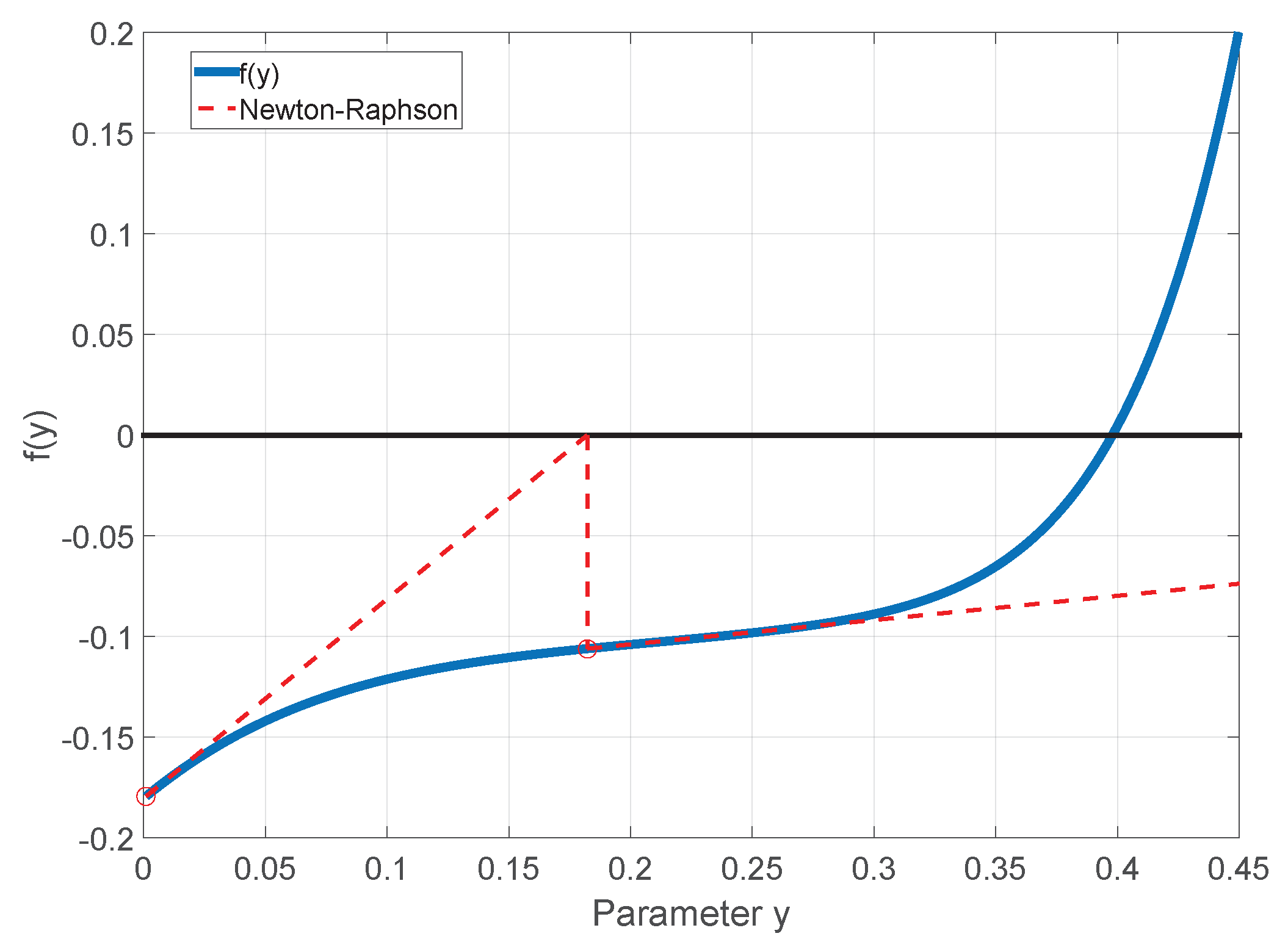
Figure 1. Example of failed solution of the H-Y method.
Energies 12 02577 g001
Figure 2. General sketch of the proposed approach.
Energies 12 02577 g002
Figure 3. The standard S-K chart and its extension to high reduced pressures.
Energies 12 02577 g003
Figure 4. Z factor values at p r = 10 for various T r values.
Energies 12 02577 g004
Figure 5. Z factor values at p r = 15 for various T r values.
Energies 12 02577 g005
Figure 6. Z factor values at p r = 30 for various T r values.
Energies 12 02577 g006
Figure 7. Performance of the TR-KRR model on the training dataset.
Energies 12 02577 g007
Figure 8. Performance of the TR-KRR model on the prediction dataset.
Energies 12 02577 g008
Figure 9. The Z factor surface generated by the TR-KRR model.
Energies 12 02577 g009
Figure 10. Examples of predicted isothermal Z factor curves vs p r .
Energies 12 02577 g010
Figure 11. Performance of four methods for the prediction of natural gas compressibility.
Energies 12 02577 g011
Table 1. Performance of the Truncated Regularized Kernel Ridge Regression (TR-KRR) model.
Training DatasetValidation Dataset
Mean error0.000.00
Mean relative error (%)0.000.00
Mean absolute relative error (%)0.040.04
Max error0.010.01
Max relative error (%)1.701.98
R 2 0.999970.99996
Table 2. Performance of the various methods on the prediction of the pipeline outlet pressure (Case Study 2).
MethodZ-Factor p out (psi)Deviation (psi)
Standing–Katz0.6950337-
Beggs and Brill0.713727859
Hall and Yarborough0.707130037
This method0.691234710
Table 3. Production data and the predicted Z-factor values at various pressure steps (Case Study 3).
P (psi)T (F) G p ( Bscf ) p pr T pr Z (B-B)Z (H-Y)Z (S-K Chart)Z (This Work)
36001500.005.481.510.8260.8420.8330.832
34501504.785.251.510.8140.8300.8220.820
330015012.655.021.510.8040.8200.8110.809
315015020.484.791.510.7950.8100.8000.798
285015038.254.341.510.7810.7940.7850.783
268515044.014.091.510.7760.7880.7800.778
Table 4. Reserves’ prediction by various methods (Case Study 3).
MethodReserves Estimate (Bscf)Deviation (Bscf)
Beggs and Brill224.44.36
Hall and Yarborough227.71.05
Standing–Katz chart228.7-
This work229.30.61