A Global Search Algorithm for Determining Water Influx in Naturally Fractured Reservoirs

Abstract
:
1. Introduction
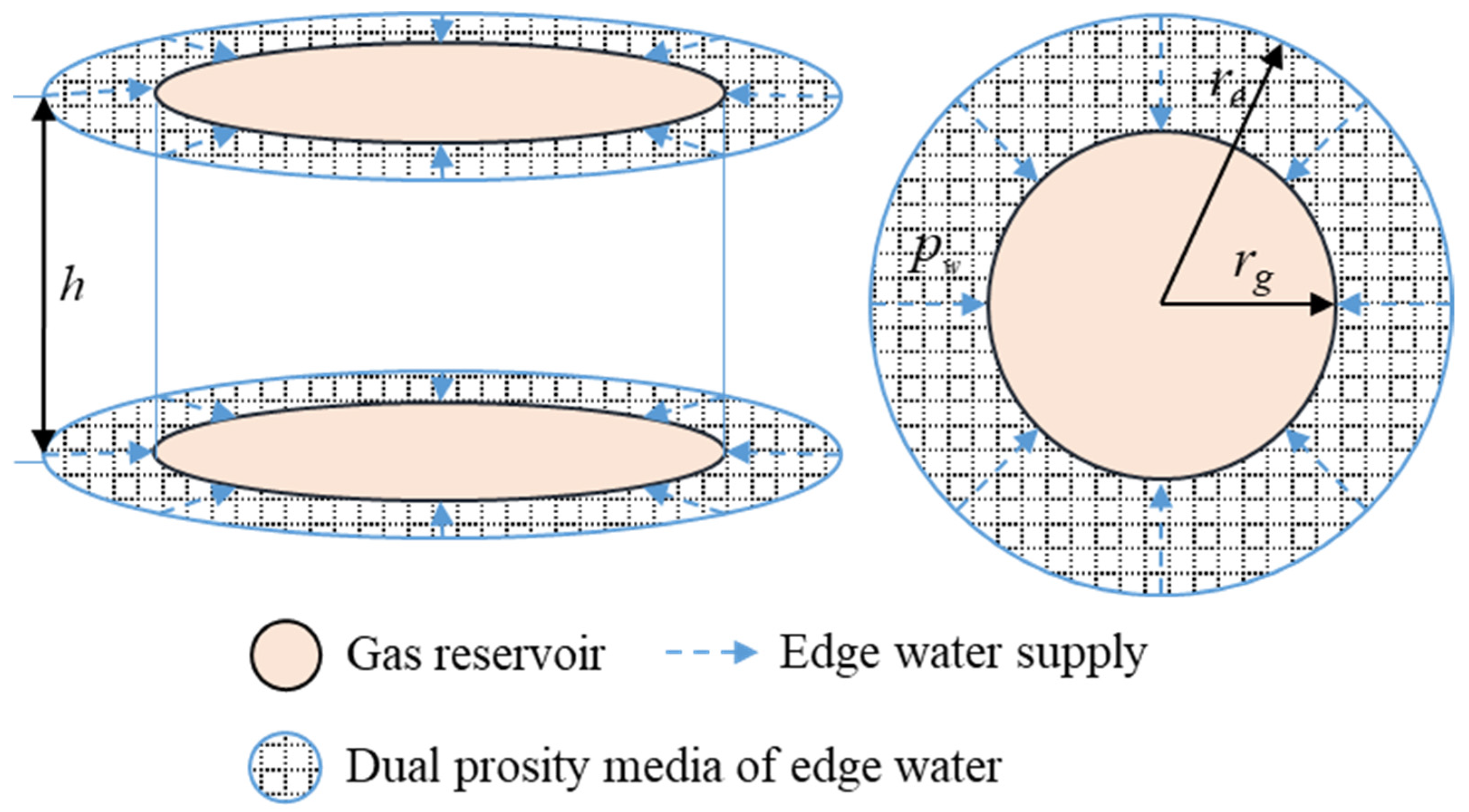
2. Conceptual Model
- The formation is equal-thick, circular and finite.
- The fluid in the aquifer is single-phase, slightly compressible and isothermal, observing Darcy’s law. The vertical flow of the fluid is ignored.
- Interflow from matrix to “wellbore” (gas reservoir) is neglected, because matrix permeability in the model is much lower than fracture permeability.
- The initial aquifer pressure is , the aquifer thickness is h, the gas reservoir radius is , and the aquifer radius is .
- The interporosity flow from natural fractures to the matrix is in the transient state in the aquifer.
3. Mathematical Model
- (1)
- The dimensionless water influx in the Laplace domain of a finite aquifer is
- (2)
- For infinite edge water, the outer boundary condition isIts seepage equations, initial conditions, and inner boundary conditions are consistent with the finite aquifer. Thus, the dimensionless water influx in the Laplace domain can be obtained by
- (3)
- The single-pore aquifer is a special case of this model, where f(s) = 1. The dimensionless water influx in the Laplace domain of a fan-shaped gas reservoir iswhere θ is the angle of water invasion in the gas reservoir in degrees (°).
4. Results and Discussions
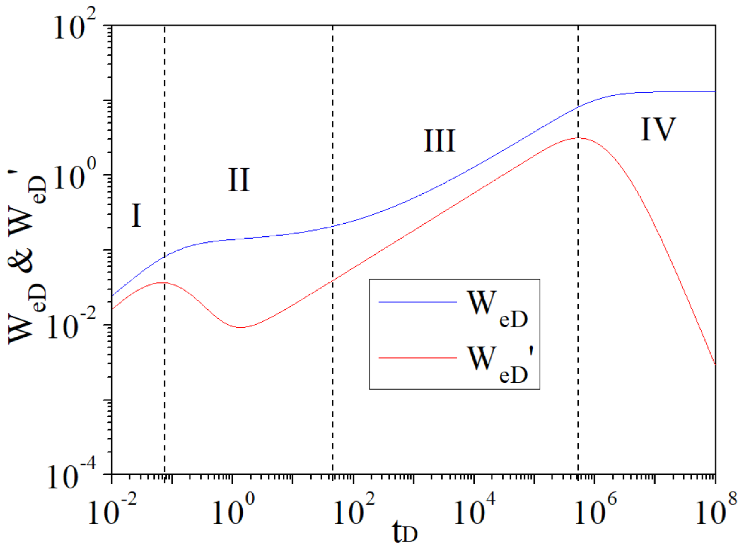
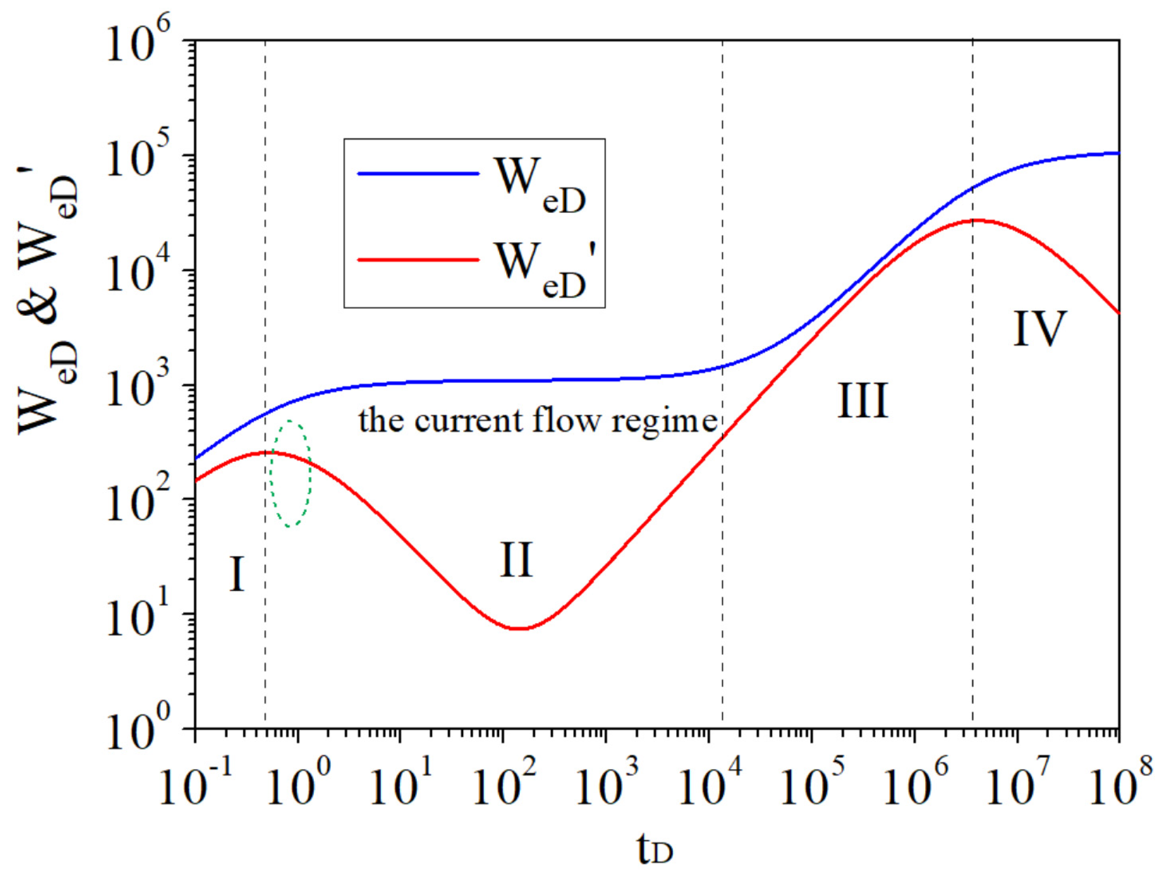
4.1. Flow Regimes
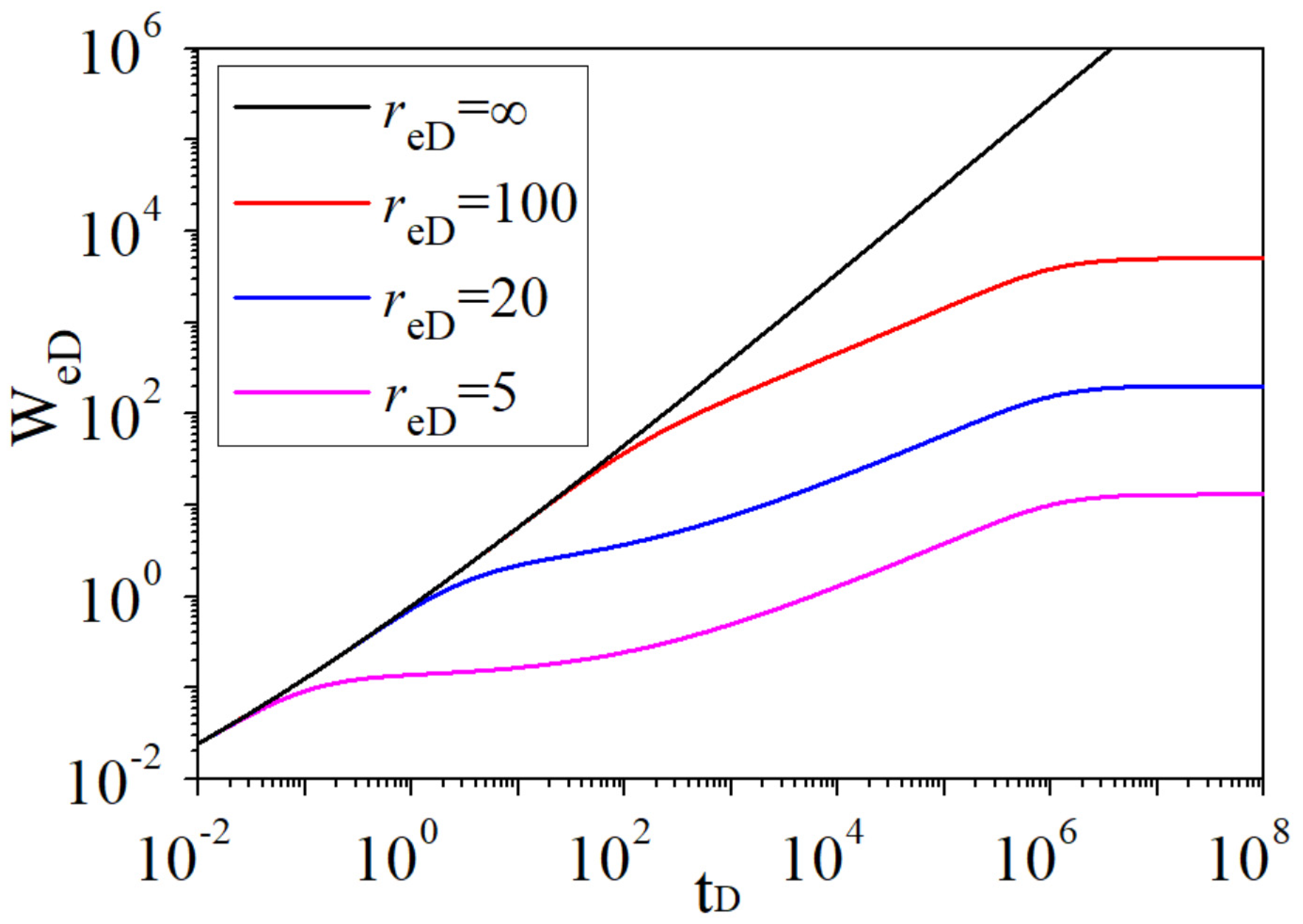
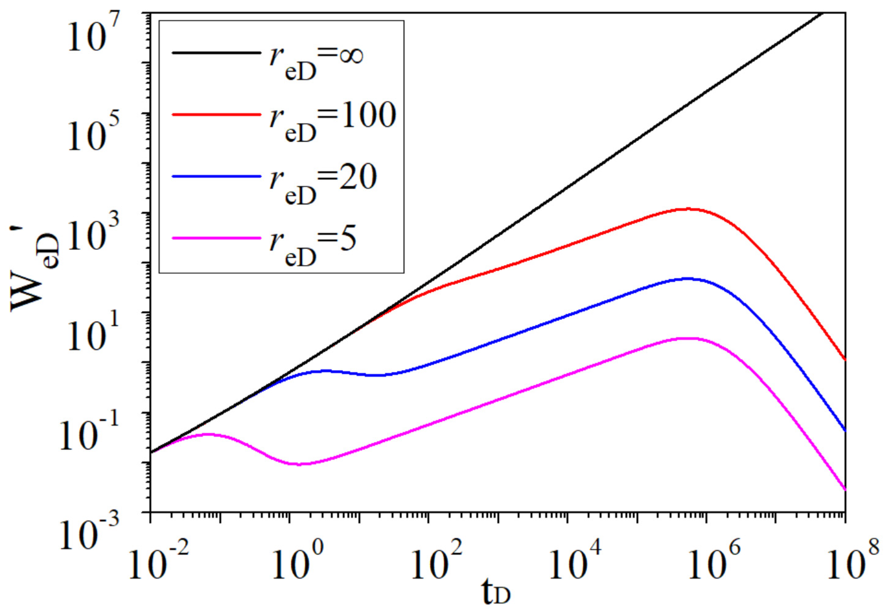
4.2. Sensitivity Study
5. Methodology
6. Field Application
7. Conclusions
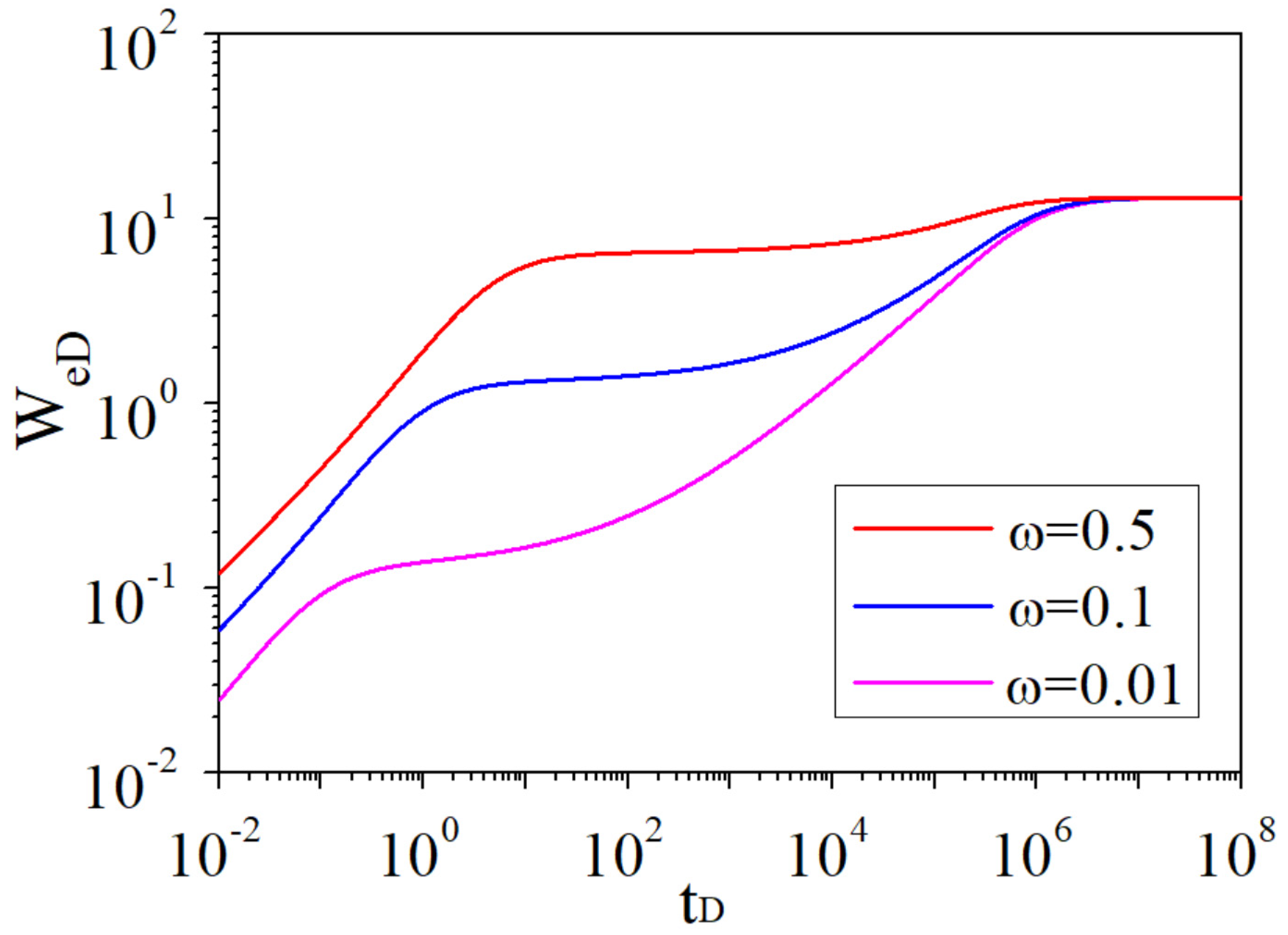
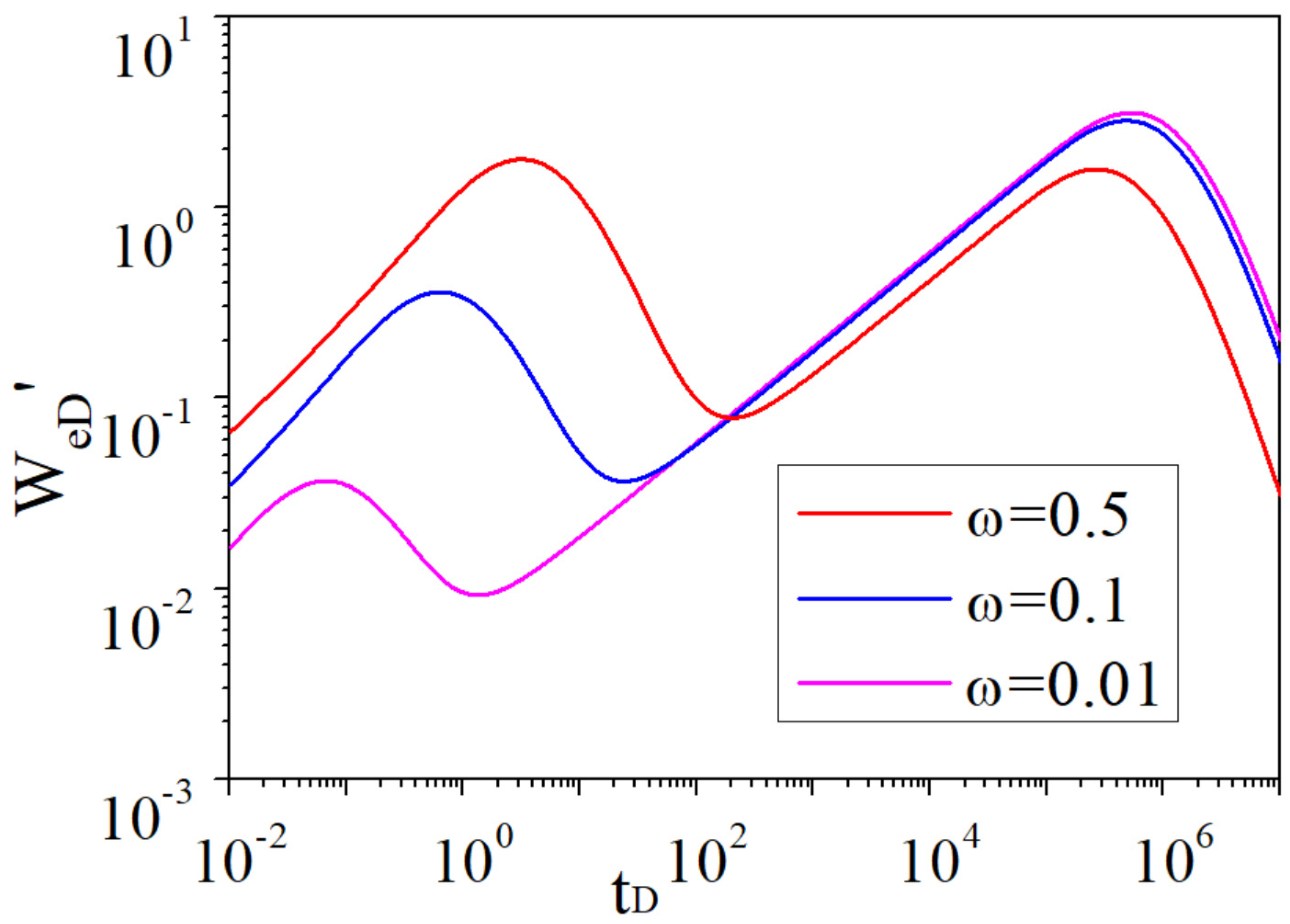
- After analyzing the water influx characteristic curves of naturally fractured reservoirs, there are four flow regimes, the water influx curves are double stepped and a “V-shape” appears in the derivative curves. For the water influx characteristic curves of homogeneous reservoirs, there are only two flow regimes, the water influx curves are single stepped and the derivative curves have no “V-shape”.
- With the decrease in the storativity ratio ω, the “V-shape” in the derivative curve appears earlier, and the difference in height between the double steps in the dimensionless water influx curve is greater.
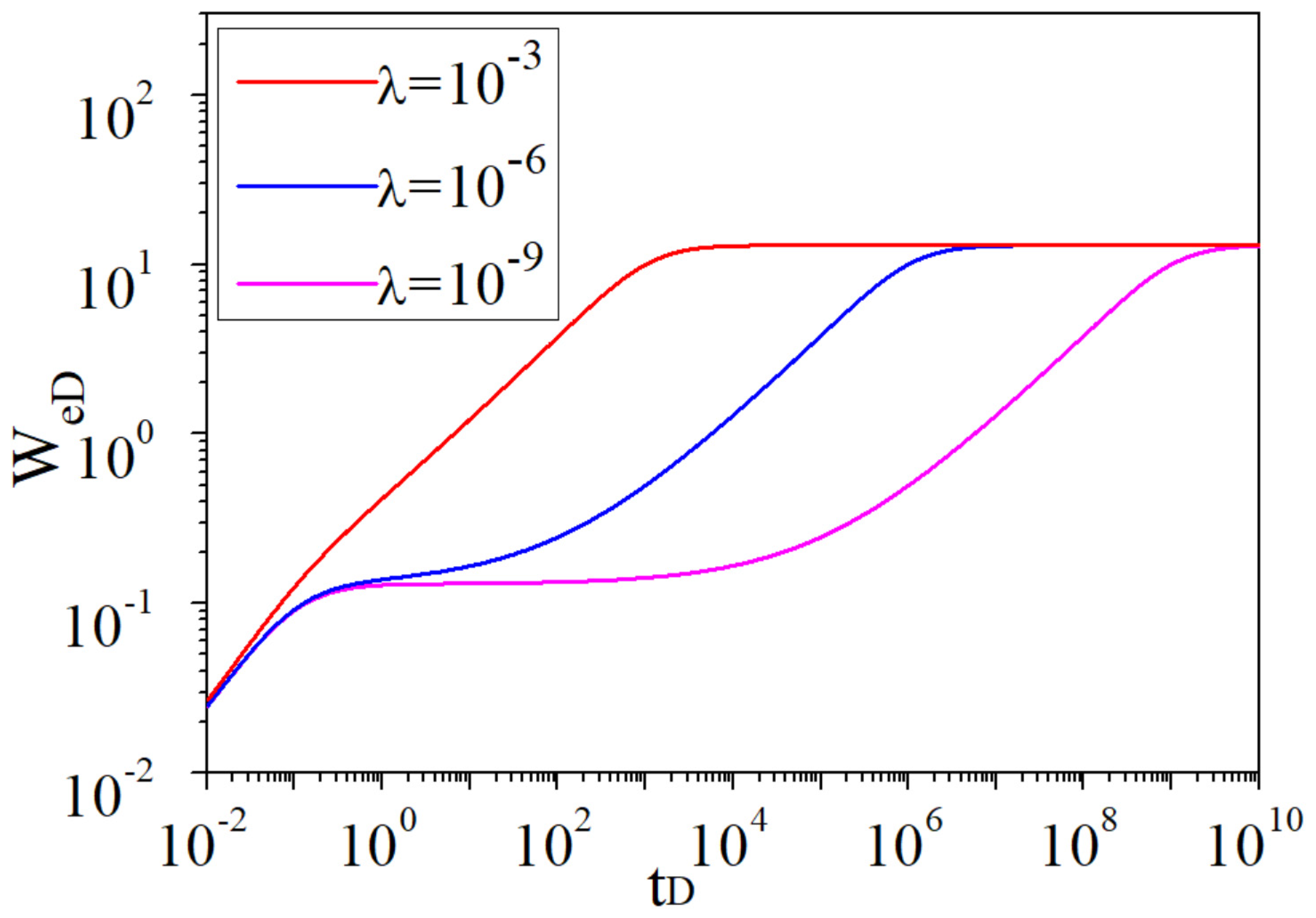
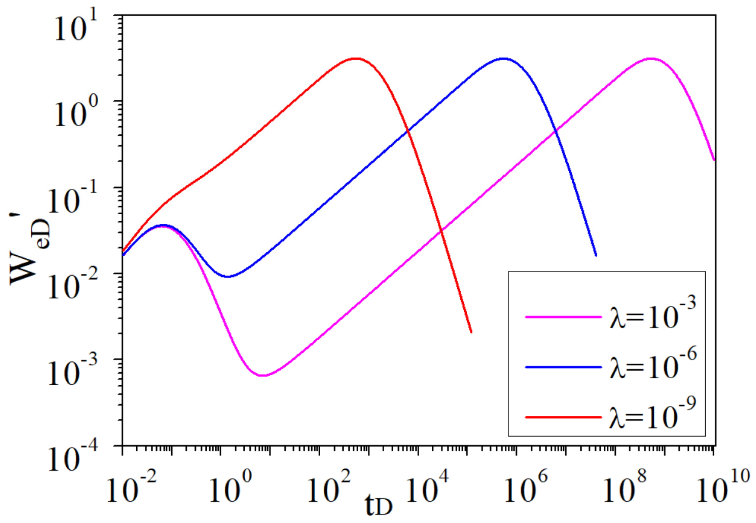
- The smaller the interporosity flow coefficient is, the more obvious the double steps in the dimensionless water influx curve and the more apparent the “V-shape” in the derivative curve are.
- The smaller the aquifer and gas reservoir radius ratio is, the more obvious the “V-shape” in the curve of the water influx derivative during the cross flow is, and the smaller the dimensionless water influx and its derivative are. These features provide meaningful tools to quantify the water influx.
- Water influx, gas radius, aquifer radius, dynamic geological reserves, and the regime of water invasion can be obtained by the global search algorithm. The results from the case study were verified by analyzing the error between dynamic and static geological reserves, and the error met the engineering accuracy, which indicates that the accuracy of the proposed method is acceptable.
Author Contributions
Funding
Acknowledgments
Conflicts of Interest
Nomenclatures
| water volume factor, m3/m3 | |
| gas volume factor, m3/m3 | |
| rock compressibility, MPa−1 | |
| formation water compression coefficient, MPa−1 | |
| comprehensive compression coefficient, MPa−1 | |
| gas reservoir volume compression coefficient, MPa−1 | |
| irreducible water saturation, dimensionless | |
| h | formation thickness, m |
| K | permeability, darcy |
| p | pressure, MPa |
| initial formation pressure, MPa | |
| q | flow flux, m3/d |
| edge water radius, m | |
| gas reservoir radius, m | |
| r | radial distance, m |
| t | time, hour |
| α | form factor, dimensionless |
| n | the number of orthogonal fracture groups, integer |
| L | the characteristic length of the rock, m |
| water influx, m3 | |
| dimensionless water influx, dimensionless | |
| Wp | the cumulative water flow flux in the ground, m3 |
| s | Laplace space operator, dimensionless |
| θ | the angle of water invasion in reservoirs, degree (°) |
| I0(x) | modified Bessel function (one class, zero order) |
| I1(x) | modified Bessel function (one class, first order) |
| K0(x) | modified Bessel function (second class, zero order) |
| K1(x) | modified Bessel function (second class, first order) |
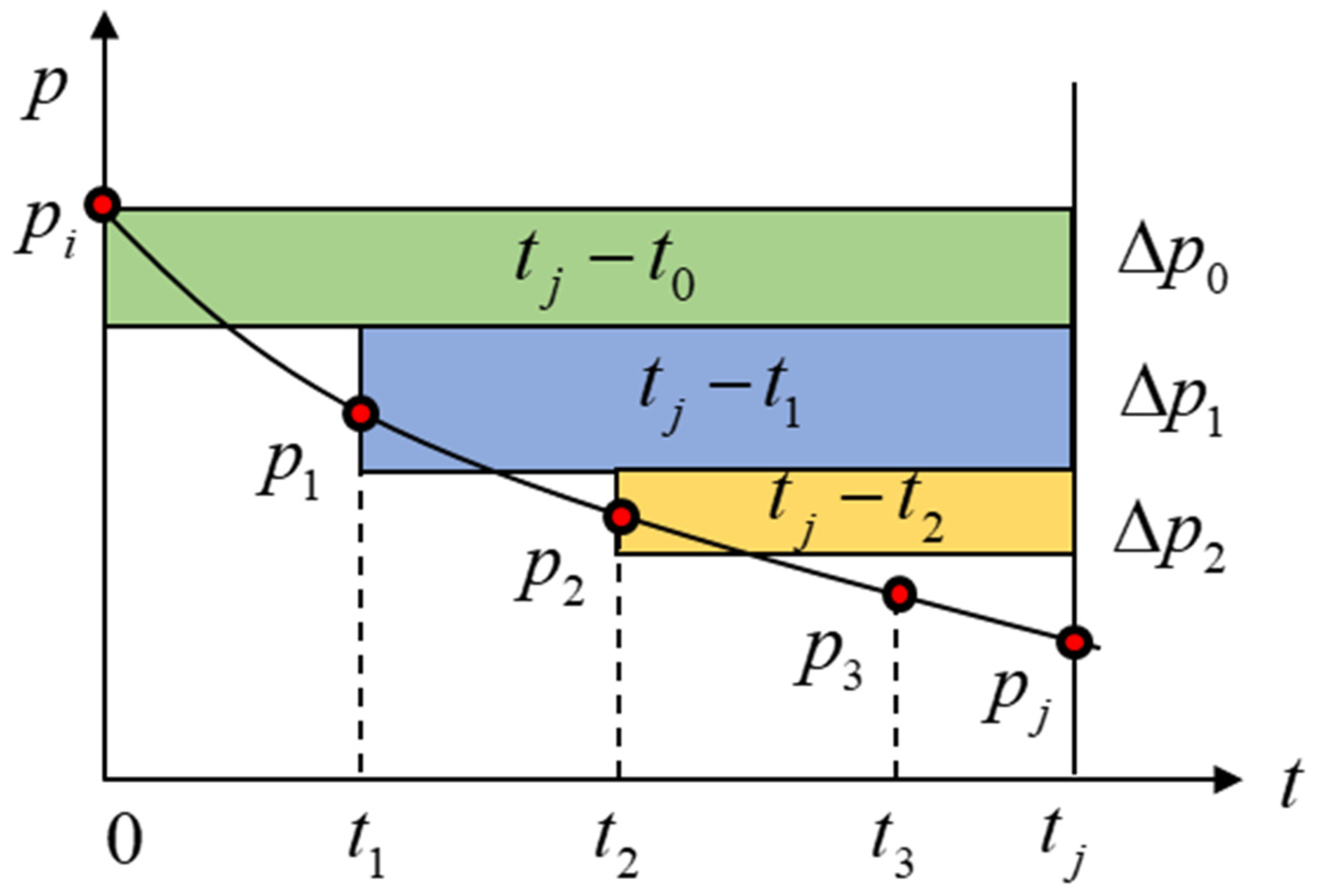
| the pressure difference at the jth stage, MPa | |
| Z | compression factor, dimensionless |
| Gp | cumulative gas flow flux, m3 |
| G | gas reservoir dynamic geological reserves, m3 |
| Gs | static geological reserves of gas reservoir, m3 |
| W | the volume of the left water in the formation, m3 |
| the H pressure of gas reservoirs, MPa | |
| the gas reservoir H pressure under original conditions, MPa | |
| e | the percentage of stored water volume in the volume of the gas reservoir, dimensionless |
| a, b | constants, dimensionless |
| T | gas reservoir temperature, K |
| Greek | |
| water viscosity, mPa·s | |
| porosity, decimal | |
| storativity ratio in aquifer, dimensionless | |
| interporosity flow coefficient in aquifer, dimensionless | |
| the error between dynamic and static geological reserves, decimal | |
| pseudo reduced pressure, dimensionless | |
| pseudo reduced temperature, dimensionless | |
| Subscript | |
| D | dimensionless |
| m | matrix |
| f | fracture |
| w | formation water |
| g | gas |
| sc | ground condition |
| Superscript | |
| − | Laplace transform |
| SI Conversion Factors | |
| MPa | ×1.0 × 106 = Pa |
| h | ×3.6 × 103 = s |
| mPa·s | ×1.0 × 10−3 = Pa·s |
| millidarcy | ×1 × 10−3 = Darcy |
| Darcy | ×1 × 10−12 = m2 |
References
- Van Everdingen, A.F.; Hurst, W. The Application of the Laplace Transformation to Flow Problems in Reservoirs. Soc. Pet. Eng. 1949, 1, 305–324. [Google Scholar] [CrossRef]
- Fetkovich, M.J. A Simplified Approach to Water Influx Calculations-Finite Aquifer Systems. Soc. Pet. Eng. 1971, 23, 814–824. [Google Scholar] [CrossRef]
- Hu, J.; Li, X.; Jing, W.; Xiao, Q. A New Method for Determining Dynamic Reserves and Water Influx in Water Drive Gas Reservoir. Xinjiang Pet. Geol. 2012, 33, 720–722. [Google Scholar]
- Liao, Z. Analysis of Outflow Rules and Production Dynamics of Fractured Water-drive Gas Reservoirs. Master’s Thesis, Southwest Petroleum University, Chengdu, Sichuan, China, 2016. [Google Scholar]
- Liao, Z.; Li, J. Review of Typical Calculation Methods for Water Influx of Water Drive Gas Reservoirs. Petrochem. Technol. 2016, 23, 117–118. [Google Scholar]
- Liu, S.; Li, Z.; Chen, P.; Guo, C.; Lai, F. A New Method for Calculating the Aquifer Influx of Abnormal High-pressure Gas Reservoirs. Spec. Oil Gas Reserv. 2017, 24, 139–142. [Google Scholar]
- Liu, T.; Huang, Q. Several Methods to Calculate Water Influx of Water Drive Gas Reservoir. Petrochem. Ind. Technol. 2016, 23, 116–125. [Google Scholar]
- Lu, K. A New Method for Water Invasion Prediction and Dynamic Reserves Calculation of Gas Cap Reservoirs. Spec. Oil Gas Reserv. 2017, 24, 89–93. [Google Scholar]
- Shimada, M.; Yildiz, T. Predicting Water Influx from Common Aquifers. In Proceedings of the EUROPEC/EAGE Conference and Exhibition, Amsterdam, The Netherlands, 8–11 June 2009. [Google Scholar]
- Song, D.; Li, X.; Nie, Y.; Xu, B. Review of Calculation Methods for Water Influx of Water Drive Gas Reservoirs. West China Explor. Eng. 2011, 23, 75–78. [Google Scholar]
- Xia, J.; Zheng, L. Calculation Method for Water Influx of Edge Water Gas Reservoir with Oil Ring. J. Liaoning Shihua Univ. 2017, 37, 30–34. [Google Scholar]
- Xu, G.; Zhu, C. Research of water production model in water encroachment gas deposit. Inn. Mong. Petrochem. 2011, 37, 172–173. [Google Scholar]
- Yu, Q.; Mou, Z.; Liu, P.; Li, Y.; Xia, J.; Li, B. Calculation Methods of Water Influx in Gas Reservoirs with Aquifers. Xinjiang Pet. Geol. 2017, 38, 586–591. [Google Scholar]
- Mcewen, C.R. Material Balance Calculations with Water Influx in the Presence of Uncertainty in Pressures. Soc. Pet. Eng. 1962, 2, 120–128. [Google Scholar] [CrossRef]
- Al-Ghanim, J.A.; Nashawi, I.S.; Malallah, A. Prediction of Water Influx of Edge-Water Drive Reservoirs Using Nonparametric Optimal Transformations. In Proceedings of the North Africa Technical Conference and Exhibition, Cairo, Egypt, 20–22 February 2012. [Google Scholar]
- Kryuchkov, S.; Moon, D.; Kantzas, A. Micro-CT Investigation of Water Influx. In Proceedings of the Canadian International Petroleum Conference, Calgary, AB, Canada, 12–14 June 2007. [Google Scholar]
- Li, Y.; Li, B.; Xia, J.; Zhang, J.; Wang, D.; Zhu, Z.; Xiao, X. New Method of Water Influx Identification and Ranking for a Super-Giant Aquifer Drive Gas Reservoir. In Proceedings of the SPE Oil & Gas India Conference and Exhibition, Mumbai, India, 24–26 November 2015. [Google Scholar]
- Li, Y.; Jia, C.; Peng, H.; Li, B.; Liu, Z.; Wang, Q. Method of Water Influx Identification and Prediction for a Fractured-Vuggy Carbonate Reservoir. In Proceedings of the SPE Middle East Oil & Gas Show and Conference, Manama, Bahrain, 6–9 March 2017. [Google Scholar]
- Chen, H.; Du, J.; Guo, P.; Liu, D.; Xiao, F.; Yang, Z. Study on Calculation of Dynamic Reserves and Water Influx in Fractured Condensate Gas Reservoir. Lithol. Reserv. 2012, 24, 117–120. [Google Scholar]
- Chen, J.; Yan, Y.; Zhang, A. Method for predicting water invasion in fractured gas reservoirs with water. Spec. Oil Gas Reserv. 2010, 17, 66–68, 123–124. [Google Scholar]
- Deng, Y.; Li, S.; Li, J. Water Invasion Performance of Fractured Gas Reservoir with Bottom-Aquifer. Spec. Oil Gas Reserv. 2016, 23, 93–95, 155. [Google Scholar]
- Li, X.; Zhang, D. Mathematical Method and Well Testing Mathematical Model; Petroleum Industry Press: Beijing, China, 1993; Volume 11, pp. 27–35, 61–96. [Google Scholar]
- Lu, D. Modern Well Test Theory and Application; Petroleum Industry Press: Beijing, China, 2009; Volume 1, pp. 44–50, 79–84, 226–246, 260–261. [Google Scholar]
- Sun, W.; Wang, S.; Yang, H.; Liu, L. Material Balance Method of Fractured Water Drive Reservoirs Considering Water Invasion Intensity. Pet. Geol. Recovery Effic. 2009, 16, 85–87, 117. [Google Scholar]
- Yang, L.; Wang, Y.; Wang, Z.; Huang, T.; Zhu, Q. Strength Estimate and the Volume Calculation for Water approaching of the Fractured Gas Reservoirs. West China Explor. Eng. 2011, 23, 43–46, 50. [Google Scholar]
- Yang, Y.; Feng, W.; Song, C. Computation Theory of Aquifer Influx in fractured edge-water drive reservoir. J. Mineral. Petrol. 2001, 21, 79–81. [Google Scholar]
- Zhou, Y.; Meng, Y.; Xu, Z.; Wang, Y.; Liang, H.; Li, G.; Zhou, H.; Wen, C. Study on the Impact of Fracture Density on the Law of Water Invasion in Tight Sandstone Gas Reservoirs. J. Chongqing Univ. Sci. Technol. Nat. Sci. Ed. 2015, 17, 13–17. [Google Scholar]
- Zhu, Z. Study on the Dynamic Law of Water Invasion of Fractured Bottom Water Gas Reservoirs. Master’s Thesis, Southwest Petroleum University, Chengdu, Sichuan, China, 2016. [Google Scholar]
- Aguilera, R. Unsteady State Water Influx in Naturally Fractured Reservoirs. In Proceedings of the Annual Technical Meeting, Petroleum Society of Canada, Calgary, AB, Canada, 12–16 June 1988. [Google Scholar]
- Warren, J.E.; Root, P.J. The behavior of naturally fractured reservoirs. SPE J. 1963, 3, 245–255. [Google Scholar] [CrossRef]
- Stehfest, H. Algorithm 368: Numerical Inversion of Laplace Transforms. Commun. ACM 1970, 13, 47–49. [Google Scholar] [CrossRef]
- Li, C. Fundamentals of Reservoir Engineering, 2nd ed.; Petroleum Industry Press: Beijing, China, 2011; Volume 9, pp. 174–184. [Google Scholar]
- Park, J.; Yang, G.; Satija, A.; Scheidt, C.; Caers, J. DGSA: A Matlab toolbox for distance-based generalized sensitivity analysis of geoscientific computer experiments. Comput. Geosci. 2016, 97, 15–29. [Google Scholar] [CrossRef]


| Parameters | Values | Units |
|---|---|---|
| Reservoir thickness | 27 | m |
| Irreducible water saturation | 0.32 | decimal |
| Formation water viscosity | 0.45 | mPa·s |
| Formation water volume coefficient | 1.01 | m3/m3 |
| Storativity ratio | 0.1 | dimensionless |
| Interporosity flow coefficient | 10−6 | dimensionless |
| Pseudo-critical pressure | 4.67 | MPa |
| Pseudo-critical temperature | 195.15 | K |
| Initial formation pressure | 29.7 | MPa |
| Initial formation temperature | 364.15 | K |
| Porosity | 0.1 | decimal |
| Natural fracture permeability | 1 | mD |
| Matrix permeability | 0.01 | mD |
| Formation water compressibility | 0.0046 | MPa−1 |
| Rock compressibility | 0.000435 | MPa−1 |
| t/mon | p/MPa | Gp/108 m3 | Wp/104 m3 |
|---|---|---|---|
| 0 | 29.7 | 0 | 0 |
| 12 | 27.4 | 6.88 | 0 |
| 20 | 25 | 17 | 120 |
| 28 | 23.7 | 27.5 | 180 |
| 36 | 21.3 | 37.3 | 260.7 |
| 48 | 19.4 | 51.5 | 500 |
| 60 | 17.6 | 61.6 | 1050 |
| We/104 m3 | ||
|---|---|---|
| 0.00 | 0.000 | 29.62 |
| 0.39 | 0.011 | 27.51 |
| 1.17 | 0.018 | 25.37 |
| 2.09 | 0.025 | 24.14 |
| 3.18 | 0.032 | 21.71 |
| 4.99 | 0.042 | 19.96 |
| 6.88 | 0.053 | 18.63 |
© 2019 by the authors. Licensee MDPI, Basel, Switzerland. This article is an open access article distributed under the terms and conditions of the Creative Commons Attribution (CC BY) license (http://creativecommons.org/licenses/by/4.0/).
Share and Cite
Zhang, J.; Liao, X.; Chen, Z.; Wang, N. A Global Search Algorithm for Determining Water Influx in Naturally Fractured Reservoirs. Energies 2019, 12, 2658. https://doi.org/10.3390/en12142658
Zhang J, Liao X, Chen Z, Wang N. A Global Search Algorithm for Determining Water Influx in Naturally Fractured Reservoirs. Energies. 2019; 12(14):2658. https://doi.org/10.3390/en12142658
Chicago/Turabian StyleZhang, Jiali, Xinwei Liao, Zhiming Chen, and Nutao Wang. 2019. "A Global Search Algorithm for Determining Water Influx in Naturally Fractured Reservoirs" Energies 12, no. 14: 2658. https://doi.org/10.3390/en12142658