On Fault Prediction for Wind Turbine Pitch System Using Radar Chart and Support Vector Machine Approach

Abstract

In order to reduce operation and maintenance cost and improve fault diagnosis and detection accuracy for wind turbines, a study on advanced methods has been carried out. The purpose of this paper is to present a new method developed using radar chart and support vector machine (SVM) approach for fault diagnosis and prediction of wind turbine pitch system as it usually has a higher failure rate. In the study, the supervisory control and data acquisition (SCADA) system data are utilized as source data for SVM prediction. First of all, the characteristics of the indicator variable data collected by the SCADA system are analyzed, and the radar charts corresponding to the normal and faulty operation of the wind turbine pitch system are constructed using the indicator variable data. Secondly, the SVM method is used to extract the gray-level co-occurrence matrix (GLCM) features and histogram of oriented gradients (HOG) features of the radar charts, and the SVM classifier is trained. Then, the operational status is predicted, the classification effect is evaluated by the confusion matrix, and the prediction evaluation index is calculated. Thirdly, the support vector regression method is used to analyze the SCADA indicator variable data, the input and output of the regression model are determined, and the training prediction model is established, and the prediction accuracy of the test model is analyzed using the test sample data. Finally, the forecasting evaluation indexes obtained by the above two methods are compared. It proves that the proposed method using SVM to analyze the system radar charts has a higher prediction accuracy of 91.24% than the support vector regression method. The prediction accuracy is improved by 8.6%. Hence, it is verified that the new method using a radar chart and SVM approach has superiority over the support vector regression method.

1. Introduction

Wind energy is one of the main renewable energy sources [1,2]. It is harvested using wind turbines and to be converted into electric power. With the increase of installed wind power capacity, more and more attention has been paid to the reduction of operation and maintenance cost. The operation and maintenance cost of wind turbines in the whole life cycle accounts for 25–30% of the total cost, e.g., Reference [3]. Failure of critical components in wind turbine operation may cause costly repairs and increased downtime. It is, therefore, that fault diagnosis and prediction has become very important. It is expected that a fault is to be detected at an earlier stage or to be predicted before it occurs [4]. The fault diagnosis and prediction are based on available data, including condition monitoring data usually collected through condition monitoring system (CMS), and control and operation data collected through the Supervisory Control and Data Acquisition (SCADA) system. CMS provides direct information reflecting a mechanical fault or failure, whereas SCADA system provides all other auxiliary information which assists in improving the efficiency and accuracy of the fault diagnosis and detection. SCADA system, for example, is an important subsystem in an energy management system which helps reduce the system operation and maintenance costs [5].

Electrical and electronic control systems in wind turbines are considered to be prone to failure, but gearbox and generator failures result in the longest downtime. In general, in large wind turbines, there are three the most vulnerable subsystems identified. They are pitch system, frequency converter and yaw system [6]. As a core component of a wind turbine, the pitch system’s failure rate is even higher than other mechanical subsystems, such as gearbox in some cases. The damage to the pitch system not only increases the operation and maintenance cost, but also reduces the production efficiency of the wind turbine [7]. In recent years, there are a number of studies reported on fault diagnosis and prediction for wind turbine pitch system, e.g., References [7,8,9,10,11,12,13,14]. Based on literature survey, it is found that the published studies can be generally classified into two categories: One is physical model-based approach, e.g., References [12,13,14,15] and the other is based on measurement data, e.g., References [16,17,18,19,20]. The physical model-based approach is mainly used for fault mechanism analysis, and the data-based studies are for condition assessment and prediction. Asgari [8] uses the unknown input observer combined with the actual operating data of the 660KW wind turbine, and detects and isolates the fault of the pitch system actuator and the generator rotor temperature rise fault in the MATLAB/Simulink environment. In Reference [9], the identification algorithm of a variable forgetting factor is introduced. Through the idea of parameter estimation, the natural frequency and damping coefficient of the variable pitch system actuator are identified and estimated, and the system fault is diagnosed by the change of parameters. Kusiak and Verma [10] established a system prediction model that is based on data mining technology for fault diagnosis of actuator failure of wind turbine pitch system. Based on the analysis of the fault characteristics of the hydraulic pitch system, Han [11] established the fault tree model of the hydraulic pitch system, and used the combination of quantitative and qualitative analysis to realize fault diagnosis. At present, the failure of the pitch system is mostly diagnosed for the mechanical failure of the system, and the diagnosis of the electrical failure of the pitch system needs to be further studied. In Reference [12], a combined adaptive and parameter estimation scheme and its application to fault prediction for wind turbines is proposed, which is based on the dynamic wind turbine and pitch system model. A set of possible faults affecting system dynamics is described. In Reference [13], a model-based variable pitch actuator fault detection method is proposed. When the pitch actuator is dynamically changed, the normalized gradient method is used to estimate the parameters of the pitch actuator and obtain the residual signal. Based on the wind farm SCADA data, Reference [14] proposed a generalized model of wind turbine anomaly identification. The fuzzy comprehensive evaluation method is used to synthesize the results of the selected wind turbine condition parameter prediction model. Reference [15] gave a method for diagnosing faults in the wind turbine pitch actuator that causes a change in pitch angle. The interval prediction algorithm is combined with recursive subspace recognition based on the variable forgetting factor algorithm. Reference [16] proposes to select more important variables in the SCADA system to improve the prediction accuracy, and adopts an index based on the exponentially weighted moving average model to eliminate the autocorrelation in the data. In Reference [17], an adaptive neural fuzzy inference system based on prior knowledge (APK-ANFIS) is proposed to analyze wind turbine SCADA data to realize automatic detection of significant pitch faults. An 85.50% classification accuracy was achieved in Reference [18] through 14 human-readable rules generated by the RIPPER induction rule learner. Of these rules, 11 were described as “useful and intuitive” by independent domain experts, and further, expert systems were developed using the model and domain knowledge. In Reference [19], for the slip ring pollution and the pitch controller failure, a novel pitch fault detection method based on performance curve (PC) normal behavior model (NBMs) is proposed. The power-generator speed (P-N) and pitch angle-generator speed (PA-N) curves were selected to establish NBMs, and behavioral curves were used to analyze behavioral differences for fault prediction. A model-based fault detection and isolation scheme for wind turbine variable pitch systems is presented in Reference [20] to detect faults in electric pitch actuators and sensors, where an Extended Kalman Filter (EKF) based multi-model adaptive estimation (MMAE) is designed to estimate the state of the system. In Reference [21], a designed algorithm based on the H2 norm optimization technique is proposed to detect blade and pitch system faults, and to repair false positive rate and detection speed as needed. In Reference [22], the fault diagnosis method of an innovative stochastic gradient algorithm based on the observer is proposed for the characteristics of wind turbine variable pitch system failure, which causes system parameters to change. The use of similar functions combined with Kohonen neural network for fault diagnosis is discussed in Reference [23] where the fuzzy clustering based on Kohonen neural network is used to solve the problem, and the optimized samples are used as input to the Kohonen network to obtain various types of standard fault models.

Generally, wind turbine fault prediction is achieved using mathematical modeling, but it is difficult to establish an accurate mathematical model because of complicated control in wind turbine operation [24]. This paper analyzes the failure of electronically controlled pitch system of wind turbines, where there are different types of failure modes. The main faults include: Blade 95-degree limit switch is triggered; pitch system charging device voltage is abnormal; blade synchronizing error; blade PMC controller output is overcurrent; blade PMC motor side grounding is short circuit; blade following error is over the limit; blade velocity controller output frequency exceeds the maximum rotational speed; blade CANbus communication error; digital channel fault of blade motor encoder; blade power detector failed; blade PMM analogue to digital converter error; pitch system input power voltage is lower; PMC controller output is overcurrent; etc. Considering that there are so many types of failure modes involved in the above-mentioned electronically controlled pitch system, it is very difficult or impossible to establish a perfect model for pitch system fault prediction. This paper proposes to follow a data-driven approach rather than a model-based approach to predicting the pitch system error in operation. Therefore, this paper starts to analyze SCADA data in order to identify the indicator variables that can reflect the majority of pitch system faults. Support vector machine (SVM) method is employed to train the prediction models by utilizing the condition monitoring and system operation data. When a failure in the electronically controlled pitch system occurs, there are seven indicators identified which reflect the change through an experimental analysis. These indicators are wind speed, wind direction, rotor speed, rotor position, output power, grid-connected frequency and pitch angle. The data of these seven indicators are extracted from a 1.5 MW wind turbine SCADA system. Then, this paper applies the method of analyzing SCADA indicator variable data to establish radar charts to perform the prediction of wind turbine pitch system failure.

2. Pitch System Data Processing

The pitch system faults account for a large proportion in the SCADA data fault list. In the predictive analysis of pitch faults, in general, only those common faults are of the focus in study and discussion. The readers are referred to the brief review given in the introduction section to learn more about the prediction methods developed. Here, we propose an innovative approach to predicting the pitch faults by using radar charts and SVM method. To apply this new approach, the first step is to collect the relevant data. In this study, one 1.5 MW wind turbine model is selected from which the SCADA system data is collected. A total of 400 data sets were collected, and classified into two groups. One group of 200 data sets represents the normal operation condition of the pitch system, whereas another group with the other 200 data sets represents the condition with the turbine pitch faults. The closer it is to the fault occurrence, the clearer it is to reflect the fault by the running and condition monitoring data. Therefore, the data representing the system condition 30 minutes before the fault occurs is collected. Through experimental analysis for testing the SVM method developed; when the wind turbine has a pitch failure, the related indicators are identified which are wind speed, wind direction, rotor speed, rotor position, output power, grid-connected frequency and pitch angle. The data collection frequency is one per 10 seconds.

Table 1. SCADA system indicator variable data when the system is in faulty operation.

Serial Number	Wind Speed (m/s)	Wind Direction (°)	Rotor Speed (rad/min)	Rotor Position (°)	Output Power (kW)	Grid Frequency (Hz)	Pitch Angle (°)
1	5.52	152.7	0.01	306.1	−10.2	50.1	0
2	3.76	130.6	0.17	300.4	−11.4	50.1	89
3	2.81	137.9	0.01	295.6	−10.2	50.1	89
4	3.05	104.4	0.01	295.3	−10.2	50.1	89
5	4.22	137.2	0.01	293.6	−10.2	50.1	89
…	…		…		…		…
179	14.79	207.6	16.7	306.2	1527	50	11.55
180	15.75	207.2	17.4	321.4	1530.6	50	16.36
181	16.87	198.6	16.4	217.6	1493.4	50	13.87

lists a set of indicator variables data—for example, when the system is in faulty operation. The negative value in the column ‘Output power’ means that there is no power output to the grid, but the wind turbine is getting power from the grid.

The data in each data set is displayed in an excel data table. Select the input quantity of indicators, including wind speed, wind direction, rotor speed, rotor position, grid-connected frequency and pitch angle, shown in a matrix table marked as I. Its dimension is 72,400 × 6. The output is output power recorded and marked as O; the dimension is 72,400 × 1. Therefore, a matrix, including input and output variable values is given in another matrix, M, M = [I, O]. The matrix table of the collected data under the pitch faulty condition is marked as I₁, and the matrix to show the normal condition data is marked as I₂. The dimension of I₁ and I₂ is 36,200 × 6. The output power data under the pitch faulty condition and normal condition are given in other separate matrixes marked as O₁ and O₂, respectively, with a dimension of 36,200 × 1. Then, there will be the matrixes $M_1=\left[I_1, O_1\right]$ under pitch faulty condition and $M_2=\left[I_2, O_2\right]$ under normal pitch condition.

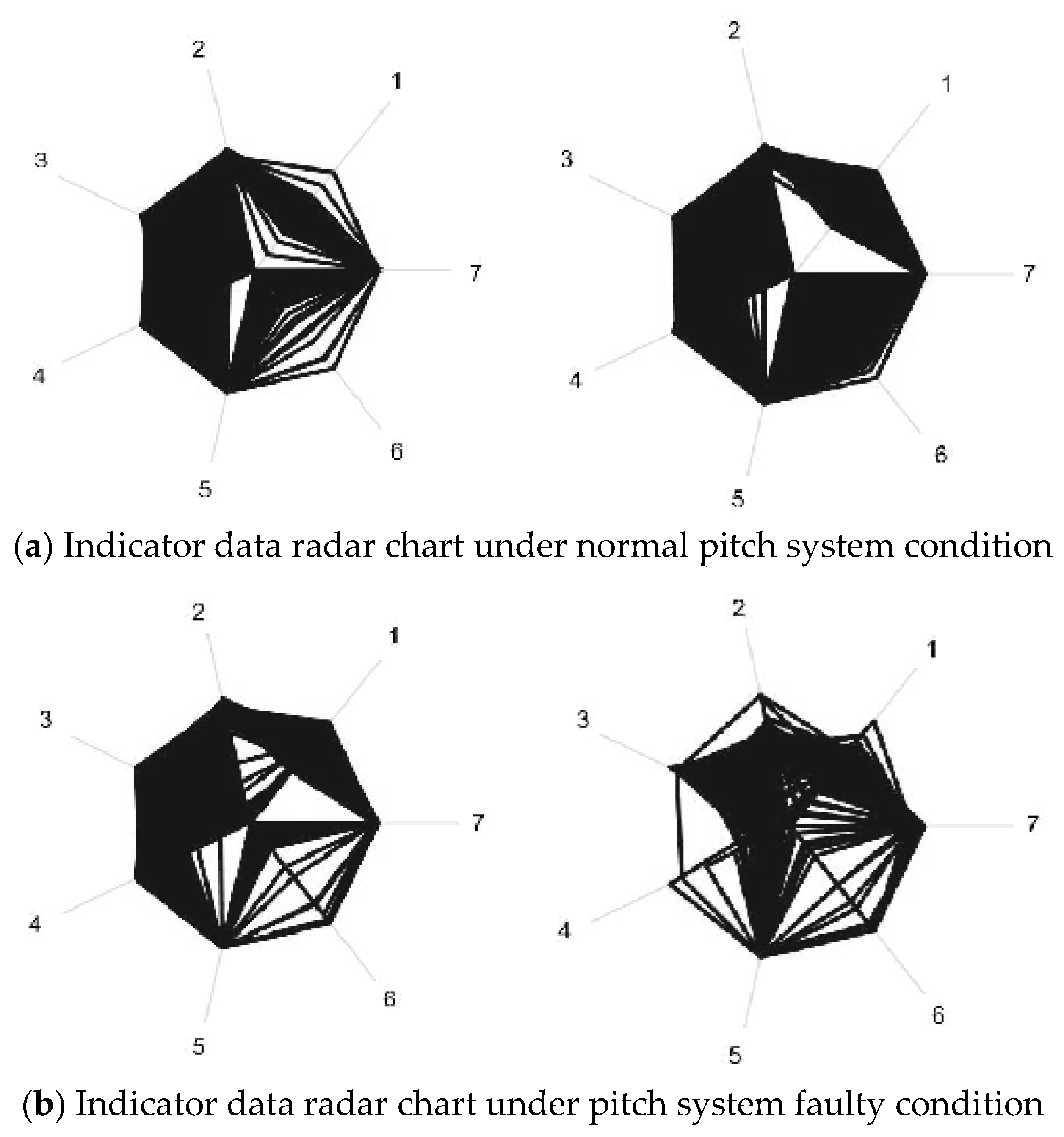
Based on the indicator variable data collected and managed as above, the radar charts corresponding to the pitch faulty and normal condition can be drawn, as shown in Figure 1. Taking the wind speed in the range from 3 m/s to 21 m/s; the radar charts with 18,001 frames corresponding to faulty and normal pitch condition are generated, respectively. The first 10,000 frames of the charts are used for training, and the remaining 8001 frames are used for testing in each. The numbers 1 to 7 in each chart represent the seven indicators in Table 1, i.e., 1 means wind speed, 2 represents indicator 2 which is wind direction; 3 means rotor speed and so on.

As can be seen from Figure 1, the radar charts of indicator variable data under normal pitch condition are more evenly distributed, and the radar charts of the indicator variable data under faulty pitch condition are less dispersed. The traditional analysis methods are based on the training analysis of fault data. This paper, however, proposes a novel analysis method based SVM for training and testing the indicator variable data radar charts under both normal and faulty pitch condition to predict the operation status of the wind turbine pitch system. Through analysis of the prediction accuracy, it is proved that the proposed method is more feasible for predicting pitch failure.

At the same time, the regression model is obtained using the training dataset data by support vector regression (SVR) method, and the prediction performance of the regression model is verified by the test set data. The predicted output power obtained by the regression model is compared with the actual output power, and the error evaluation indices are calculated to analyze the operational status of the pitch system.

3. Forecast Method Analysis

3.1. Indicator Variable Data Radar Chart Forecast by SVM

SVM is a machine learning method with supervised features, which improves the generalization ability of machine learning through structural risk minimization [25]. The empirical risk and confidence interval are minimized, and the pattern classification is effectively performed by extracting the characteristics of the radar chart drawn using the data of related indicators.

Figure 2 below shows the flow diagram of the algorithm for processing image classification using SVM. The flow chart mainly includes extraction of the image features, SVM classification operation, sample prediction and surface classification effect through the confusion matrix. First, the input picture is converted into a grayscale image, the image gray-level co-occurrence matrix (GLCM) feature is extracted and normalized, and then the grayscale image is binarized. The image histogram of oriented gradients (HOG) features are extracted, and the GLCM features and HOG features are combined as feature vectors of the image, and the algorithm outputs are characteristics and tags of the training set and the test sets. Secondly, the SVM classifier is trained by the obtained image features. Then, the prediction of the sample tag is performed using the feature vector of the test image. Finally, the classification effect is evaluated through a constructed confusion matrix.

3.1.1. Image Feature Extraction

The indicator variable data radar charts under normal operation and pitch faulty operation have differences in their shape characteristics. It is to predict the indicator variable values under normal operation and pitch faulty condition by extracting the image GLCM feature and HOG feature in this paper. Before performing feature extraction, the RGB color space image is first converted into a gray image, and the gray image is converted into a binary image by setting a threshold. The threshold is set to be 0.5608.

For Grayscale image GLCM feature extraction, it is noticed that the indicator variable data radar charts under normal operation and pitch faulty condition have different grayscale features. Here, the average value and variance are taken as the final extracted features of the image, and the mean value indicates that the degree of brightness to darkness of the image. The variance is used to display grayscale contrast. The larger the variance value is, the greater the grayscale contrast of the image is.

3.1.2. Constructing Confusion Matrix

This paper evaluates the classification effect of the algorithm by constructing a confusion matrix. The confusion matrix presents the visualization effect of the performance of the algorithm through a specific matrix, which is a situation analysis table that summarizes the prediction results of the classification model in machine learning. In the evaluation, the following terms are used: TP (True Positive) means that the true value is true and the predicted value is true; FN (False Negative) means that the true value is true and the predicted value is false; FP (False Positive) means that the true value is false and the predicted value is true; and TN (True Negative) means that the true value is false and the predicted value is false. Then, the prediction performance is evaluated by the following five indices:

(1)

Diagnostic accuracy

$$Diagnostic Accuracy=\frac{TP+TN}{TP+TN+FP+FN}$$

(1)

It is the most important indicator for evaluating a fault diagnostic model.

(2)

Predicted as true accuracy

$$Precision=\frac{TP}{TP+FP}$$

(2)

It is the proportion of the positive class records that the classifier judges to be in positive class.

(3)

True to true accuracy

$$Recall=\frac{TP}{TP+FN}$$

(3)

Recall represents the proportion of positive samples whose metrics are correctly predicted by the classifier.

(4)

True to false accuracy

$$Specificity=\frac{TN}{TN+FP}$$

(4)

Specificity indicates the ratio of the number of faults being correctly diagnosed to the actual number of faults, and it reflects the fault diagnosis capability of the model.

(5)

Predicted as false accuracy

$$Negative\mathrm{Pr}ediction=\frac{TN}{TN+FN}$$

(5)

Negative Prediction indicates the proportion of times when the fault is correctly diagnosed as a fault, which indicates the credibility of the diagnosis as a fault.

3.2. Support Vector Regression Prediction

SVR is the application of SVM to regression problems [26]. SVR can deal with practical problems, such as small samples, nonlinear and high digits, and can be effectively applied to modeling and prediction of nonlinear data and even optimization control. At the same time, it overcomes the issues that network structures, such as neural networks are difficult to determine, and it is prone to fall in local convergence so as to turn out the local extreme points [27].

When using SVR to handle regression problems for a given sample set {$\left(x_i, y_i\right)$} (i = 1, 2, Λ, M), $x_i$ is the ith m-dimensional input vector, $y_i$ is the ith output vector and M is the sample size. Through a function, g(x), the m-dimensional input vector is mapped into the l-dimensional feature space, l > m. The SVR implementation constructs a hyperplane $f\left(x\right)={\omega }^{T}g\left(x\right)+b$ in the feature space, where $\omega$ is the l-dimensional weight vector, and b is the bias term. The purpose is to obtain the distance $\left|y_i-f\left(x_i\right)\right|$ < ε from all sample points to the hyperplane, where ε is the given precision. When the error is less than ε, it is not considered. When the error is greater than ε, the extra error is usually expressed by the relaxation factors ξ and ξ*.

According to the structural risk minimization criterion, the optimization objectives and constraints of the SVR model are expressed, respectively, as follows [28]:

$$\underset{\omega ,b,\xi ,{\xi }^{*}}{\min }\left\{\frac{1}{2}{\Vert \omega \Vert }^2+C{\displaystyle \sum _{i=1}^M({\xi }_i+{\xi }_i^{*})}\right\},$$

(6)

$$subject to\{\begin{array}{c}{y}_i-f\left(x_i\right)\le \epsilon +{\xi }_i,\hspace{1em}i=1,\dots M.\\ f\left(x_i\right)-y_i\le \epsilon +{\xi }_i^{*},\hspace{1em}i=1,\dots M.\\ {\xi }_i\ge 0,{\xi }_i^{*}\ge 0,\hspace{1em}i=1,2,\dots ,M.\end{array}$$

where, ε ≥ 0 is the fitting accuracy of the function; ${\xi }_i$ ≥ 0 and ${\xi }_i^{*}$ ≥ 0 are the relaxation factors; and C > 0 is used to control the degree of penalty for the sample exceeding the error, ε.

The non-negative Lagrangian multipliers ${\alpha }_i$ and ${\alpha }_i^{*}$ are introduced by the objective function and the corresponding constraints, and the Lagrange function is constructed to transform the Equation (6) as:

$$\underset{\alpha ,{\alpha }^{*}}{\max }\left\{-{\displaystyle \sum _{i=1,j=1}^M\left({\alpha }_i-{\alpha }_i^{*}\right)}\cdot \left({\alpha }_j-{\alpha }_j^{*}\right)g^T\left(x_i\right)g\left(x_j\right)-\epsilon {\displaystyle \sum _{i=1}^M\left({\alpha }_i+{\alpha }_i^{*}\right)}+{\displaystyle \sum _{i=1}^M{y}_i\left({\alpha }_i-{\alpha }_i^{*}\right)}\right\},$$

(7)

$$subject to\hspace{1em}{\displaystyle \sum _{i=1}^M\left({\alpha }_i-{\alpha }_i^{*}\right)}=0\hspace{1em}0\le {\alpha }_i,{\alpha }_i^{*}\le C.$$

By solving Equation (7), the optimal hyperplane function is obtained,

$$f(x)={\displaystyle \sum _{i=1}^M({\alpha }_i-{\alpha }_i^{*})}{g}^T\left(x_i\right)g\left(x\right)+b.$$

(8)

An important concept in this model is the kernel function. From the Mercer theorem, this kernel function is:

$$K(x_i,x)=g^T(x_i)\cdot g(x).$$

(9)

Thus, insert Equation (9) into Equation (8), the optimal hyperplane function is changed to:

$$f(x)={\displaystyle \sum _{i=1}^M({\alpha }_i-{\alpha }_i^{*})}K(x_i,x)+b.$$

(10)

Equation (10) is the SVR function. Figure 3 gives a flow diagram showing the SVR prediction modeling algorithm. It starts with the determination of the input and output variables of the model like the seven indicators selected, then select a kernel function and regression parameter values, such as the kernel function is selected as a linear function f(x) = ω^T·x + b and C = 2.2 based on a preliminary study. After that, do sample data pretreatment, that is, the indicator variables data are organized and put into a designed table in excel spreadsheet like Table 1, for instance. The data is then grouped into two groups as training data and testing data, for example, 75% of the data is used for training model, and the remaining 25% is used for testing the model. Train the model until the model evaluation criteria, $R^2$ and RMSE values are satisfied, i.e., $R^2$ is larger than the threshold and RMSE is less than the setting target. After the model is obtained, it is tested using the test sample data.

Root Mean Squared Error (RMSE) is calculated by:

$$RMSE=\sqrt{\frac{1}{n}{\displaystyle \sum _{i=1}^n{(f(x_i)-y_i)}^2}}.$$

(11)

The model determination, R² (Square correlation coefficient) is calculated by:

$$R^2=\frac{{(n{\displaystyle \sum _{i=1}^{n}f(x_i)}{y}_i-{\displaystyle \sum _{i=1}^{n}f(x_i)}{\displaystyle \sum _{i=1}^n{y}_i})}^2}{\left(n{\displaystyle \sum _{i=1}^{n}f{(x_i)}^2}-({\displaystyle \sum _{i=1}^{n}f(x_i){)}^2}\right)(n{\displaystyle \sum _{i=1}^n{y}_i{}^2}-{({\displaystyle \sum _{i=1}^n{y}_i})}^2)}.$$

(12)

In Equation (12), $y_i$ is the ith true value; $f\left(x_i\right)$ is the ith simulated output value; n is the total number of test data.

4. Prediction Results and Analysis

In order to verify the effectiveness of the SVM algorithm, the radar charts are processed first, to achieve the radar charts of the indicator variable data under pitch system normal and faulty operation condition, followed by feature extraction. Finally, the SVM training model is used to generate the confusion matrix and analyze the prediction indices.

At the same time, the SVR model is established for the normal operation of SCADA data. For different operating conditions, the actual output power and the output power of the training model are compared to obtain the SVR model prediction accuracy.

By comparing the prediction effects of the above two methods, the feasibility and efficiency of using the SVM to forecast the wind turbine pitch system under normal and faulty condition are verified using the real wind turbine operation data in production.

4.1. SVM for Graphics Prediction and Prediction Accuracy Analysis

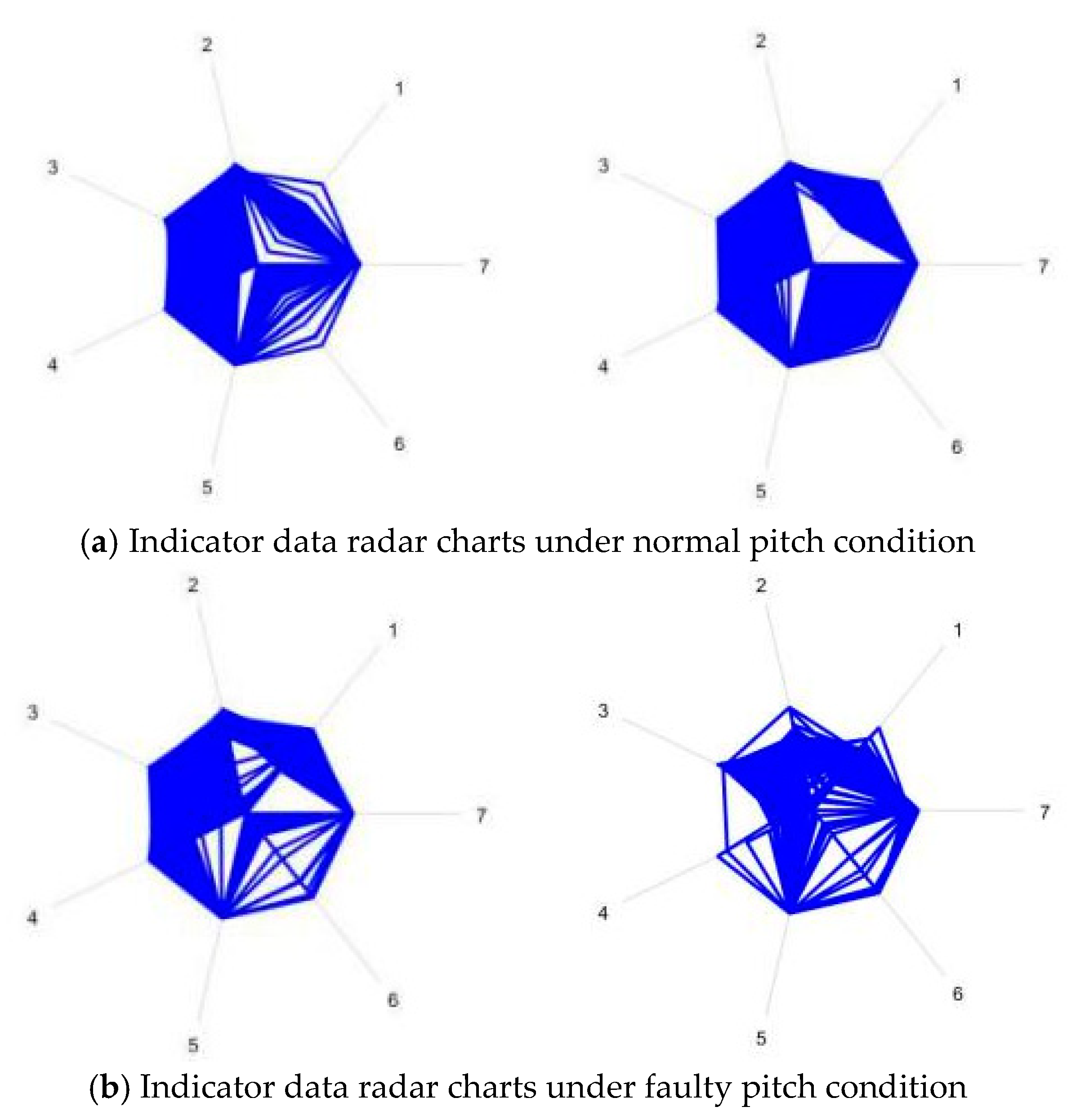
The SVM algorithm is used to perform fault prediction on the generated radar charts under different operation states of the wind turbine using the data collected. The radar charts plotted with the indicator variable data are shown in Figure 4. First, the radar image is grayscale processed, and the GLCM features of the image are extracted, and the average and variance are taken as the final extracted features of the image. The HOG features of the radar charts are then extracted, and the GLCM features and HOG features are combined as feature vectors of the image. After the SVM is trained, the classification effect of the model is evaluated by the generated confusion matrix.

4.1.1. Image Feature Extraction

(1) Image Grayscale Processing

Before extracting the characteristics of the radar chart, the graphics are first grayscaled, as shown in Figure 4.

(2) Image Feature Extraction

Here, the average value and the variance are used as the GLCM features of the extracted image. Since there are too many image samples and it is difficult to observe the feature difference, we select 150 sample charts from normal pitch system operation and 150 sample charts from when the system is in faulty condition to make a comparison in mean and variance of the GLCM features of the extracted image. The numbers 1–7 in Figure 4 represent the seven indicators in Table 1.

Figure 5 shows the GLCM feature average of grayscale values of the images for comparison. The feature extraction of the radar charts is from four directions, θ = 0°, 45°, 90°, 135°; and the 150 average values of the radar charts when the pitch system is in normal and faulty condition are calculated. Similarly, Figure 6 shows the comparison of GLCM feature variance of grayscale values of the images in these four directions.

As shown in Figure 5 and Figure 6, there is only a small or no overlap of the mean value and variance of the GLCM feature of the radar charts under two different conditions, the wind turbine pitch system faulty and normal operation status can be clearly distinguished. Obviously, the mean value of the feature under wind turbine faulty condition, as shown in Figure 5, is lower than the normal operation status except for the 0° direction; and the value under normal operation status in Figure 6 is always higher than the faulty condition. This provides a basis for the prediction of the subsequent operational status, i.e., normal operation or faulty condition.

4.1.2. Forecast Index Value Calculation

According to the construction of the confusion matrix, the values of the prediction indices, TP, FN, FP, and TN are shown in

Table 2. Forecast index value.

Index	TP	FN	FP	TN
Value	6599	1402	0	8001

. According to the prediction index values obtained, the prediction accuracy, the accuracy that the prediction is true, the true-true accuracy, the true-false accuracy and the accuracy that the prediction is false, are shown in

Table 3. Forecast evaluation index value.

Index	Accuracy	Precision	Recall	Specificity	Negative Prediction
Value (%)	91.24	100	82.48	100	85.09

below.

4.2. SVR Model Training and Prediction Accuracy Analysis

The input data is processed separately before performing predictive network training. The data is organized in the same way as described in Section 2, such as the data table is expressed as M, denoted as M = [I, O]. The indicator variable values corresponding to the pitch system faulty condition is given in another table, which is denoted as M₁ = [I₁, O₁]. Following the same, we have M₂ = [I₂, O₂] for the indicator variable data under the system normal operation. The input variable matrix dimension is 36,200 × 6, and the output vector dimension is 36,200 × 1 for each M₁ and M₂.

Starting from the first line of M₁ and M₂, take one line in every three lines and generate an array with the dimension of 9050 × 7 as the test data set of the model, denoted as N₁ and N₂. Starting from the first line of M₁ and M₂, take three lines every other line to generate another array with the dimension of 27,150 × 7 as the training data set of the model, denoted as N₃ and N₄.

The architecture of the SVM is shown in Figure 7, where K is the kernel function [29].

The idea to use the kernel function is to transform the random vector X_i on the feature space into a high-dimensional feature space F by nonlinear Φ mapping. Hence, it is to get a solution in high-dimension space by linearly dividing the space. The mapping is shown below:

$$\begin{array}{c}\mathsf{\Phi }:R\to F\\ X_i\to \mathsf{\Phi }(X_i)\end{array}.$$

(13)

In this paper, the linear kernel function C-SVR model is used, and the linear function f(x) = ω^T·x + b is applied for data fitting. For the optimization problems given in Equations (6) and (7); M, ${\alpha }_i$ and ${\alpha }_i^{*}$ are the Lagrange multipliers corresponding to the original problem with inequality constraints. The corresponding fitting function is f(x) = ω^T·x + b = ${{\displaystyle \sum }}_{i=1}^M\left({\alpha }_i^{*}-{\alpha }_i\right)\left(x_i·x\right)$ + b.

Setting error interval as [−6, 6] and the step size 0.5, it is used to record the number of errors that fall in each area. By taking the normal training data as an example, the number of errors distributed in each interval is obtained as PP_normal_train, then the error value in each region is averaged to obtain PP_normal, and finally, the three-term polynomial curve fitting is used to obtain PP_normal_result. For abnormal training data, normal test data, and abnormal test data; the same results are obtained through fitting as PP_fault_result, PP_normaltest_result, and PP_faulttest_result. The normalized data and abnormal data are tested on the trained network to verify the network prediction accuracy. The verification is by the following equation,

$$\begin{array}{l}{J}_1={\left(PP\_normal\_result-PP\_normaltest\_result\right)}^2\\ J_2={\left(PP\_fault\_result-PP\_faulttest\_result\right)}^2\end{array}$$

(14)

Y = J₁/J₂ is the threshold which is set to be 0.85 in this paper. When Y < 0.85, the output value is recorded as 0 to indicate normal operation. When Y ≥ 0.85, the output value is recorded as 1 to represent the faulty operation condition. A threshold of 0.85 is more stringent than a threshold of 1 to avoid missing some faults. However, as the turbine system is working under dynamic load and operates under different operating conditions, the value setting needs to be carefully considered.

4.2.1. Output Power Comparison

Figure 8 below gives a comparison of the output power of the training model and the actual output power. Figure 8a shows the comparison between the normal training output power and the model predicted output power; Figure 8b presents the comparison between the abnormal training output power and the model predicted output power; Figure 8c shows the comparison between the output power of normal test and the model predicted output power; and Figure 8d gives comparison between the abnormal test output power and the model predicted output power.

4.2.2. Error Index Comparison

The error indices are error integral (IE), absolute error integral (IAE), and squared error integral (ISE), which are used in comparing the normal training output power with the model predicted output power, the abnormal training output power and the model predicted output power, the normal test output power and the model predicted output power, and the abnormal test output power and the model predicted output power. The calculated error indices are given in

Table 4. Actual output power and model training output power error index.

Data Set Status	IE	IAE	ISE
Normal training	2.871	11.426	2.452 × 103
Abnormal training	−49.059	66.378	6.799 × 104
Normal test	13.775	17.386	5.576 × 103
Abnormal test	−29.952	39.120	3.465 × 104

in the case study. It can be seen from the table that the error value obtained by the SVR analysis is within an acceptable range.

4.2.3. Forecast Index Calculation

The SVR performs a regression analysis to obtain the prediction indices TP, FN, FP, and TN values, as shown in

Table 5. Forecast index value.

Index	TP	FN	FP	TN
Value	6804	2246	896	8154

below.

According to the prediction data obtained above, the prediction accuracy is evaluated, they are the accuracy of prediction, the accuracy that the prediction is true, the accuracy of the true to be predicted as true, the accuracy of the false to be predicted as false, and the accuracy of that the prediction is false, as shown in

Table 6. Forecast evaluation index.

Index	Accuracy	Precision	Recall	Specificity	Negative Prediction
Value (%)	82.64	88.36	75.18	90.09	78.40

.

4.3. Comparison between Prediction Methods

The prediction results using the SVR model and the SVM on the image prediction model are compared. The results of the index comparison are shown in

Table 7. Forecast evaluation index.

Approach	Accuracy	Precision	Recall	Specificity	Negative Prediction	False Alarm Rate
SVM Model Prediction (%)	82.64	88.36	75.18	90.09	78.40	17.36
SVM processing graphics (%)	91.24	100	82.48	100	85.09	8.76
Accuracy improvement (%)	8.60	11.64	7.30	9.91	6.69	8.60

.

It should be noted, False alarm rate is the rate that wind turbine system health status is predicted/forecasted wrongly, it is False alarm rate = 1 − Accuracy.

It can be seen from Table 7 that using SVM to analyze the radar chart, the accuracy of the training prediction model is higher than that of the regression model using SVR. The accuracy of the SVM training prediction model is 8.6% higher than that of the SVR prediction model. It is found that the true accuracy rate is 11.64% higher, the true-true accuracy rate is 7.3% higher, and the true-false accuracy rate is 9.91% higher, the false accuracy rate is 6.69% higher, and the predicted false alarm rate was reduced by 8.6%.

4.3.1. Comparison of Model Prediction Accuracy Using Regression and Neural Network Approach

In a previous study [30], multivariate linear regression and BP neural network were used to predict the wind turbine pitch system failure, caused by pitch 3° position sensor failure, pitch 90° position sensor failure, un-synchronizing of three blade position in pitching, pitch in emergency mode, pitch safety chain failure and pitch motor over-temperature using the data collected from the same wind farm. The seven indicator variables data were extracted from the collected data set to construct a model for analysis. Then, the pitch failure prediction model performance indices are shown in

Table 8. Pitch failure model prediction performance index.

Approach	Accuracy	Error	Specificity	Negative Prediction
Multiple linear regression analysis (%)	71	29	70	71.4
BP neural network analysis (%)	83	17	82	83.7

. It is found that the BP neural network prediction model is better than the multivariate linear regression analysis in terms of fault detection ability.

Similarly, in our another study [31], BP neural network and wavelet BP neural network were applied to model development for prediction of wind turbine pitch system failure caused by several other failure modes, including the pitch was in emergency mode, the pitch safety chain failed, three blades were not synchronized, the blade was not able to be reciprocated, the pitch communication was off, and blade hit 95° limit, using the data collected in the same time period as in the above comparison analysis. The prediction accuracy by the two approaches is shown in

Table 9. Pitch failure model prediction performance indices.

Approach	Accuracy	Error	Specificity	Negative Prediction
BP neural network analysis (%)	65	35	64.2	68
Wavelet BP Neural Network analysis (%)	82	18	79.6	86

. It is clearly identified that the wavelet BP neural network prediction accuracy is higher than the BP neural network model.

4.3.2. Summary and Discussion

Based on the above comparison analysis of the competitive models for prediction of pitch system failure, it has been found that the SVM method based on the radar charts generated using the relevant indicators data extracted from the collected wind turbine operation and monitoring data sets provides the best performance in prediction of pitch system failure than other competitive approaches. The prediction accuracy in terms of pitch system fault is as high as 91.24%, which is clearly higher than other models developed using multivariate regression and Neural Network techniques. The main reason may be due to the advantages of the SVM method as discussed below:

(1) For the fault prediction of wind turbine pitch control system, the image processing accuracy is higher than the data processing accuracy. In this study, the SVM is used to process the generated radar charts, and SVR is based on the recorded data so that the prediction accuracy using the SVM method is higher than using SVR.

(2) SVM is a novel small sample learning method with a solid theoretical background. In essence, it avoids the traditional from induction to deduction process, and can achieve efficient "transduction reasoning" from training samples to forecast samples, which greatly simplifies the general classification and regression process in problem solution.

(3) In general, a small proportion of support vectors determine the final result in a prediction analysis. This tells us to search for and grasp the key samples among a large number of redundant samples so that the developed algorithm shall be simple and show good “robustness”. The SCADA system collects a large amount of data, and it inevitably involves redundant and useless information, which will cause interference to the training model. For this reason, SVM is used for classification in this study.

(4) It is finally to solve a convex quadratic programming problem. In theory, we will get the globally optimal solution and solve the issue with local extremum with SVW, which is, however, hardly avoided in the neural network method.

Although it is known that it is difficult to solve the multi-classification problem with SVM, the focus of this research is on binary-pattern classification, so that it does not involve this issue.

5. Conclusions

In this paper, the SVM method is utilized to process the radar charts generated using the wind turbine pitch system operation indicators data collected. The data representing the wind turbine pitch system under normal operation condition and faulty condition were collected, and the corresponding radar charts were plotted. In the analysis, it is first to make the radar image grayed out, and the average value and variance of the gray image GLCM feature extracted are calculated. The HOG features are extracted after binarization, and the GLCM features and HOG features are combined as feature vectors of the image. Then the SVM prediction model is trained, and finally, the prediction accuracy of the prediction model is evaluated using the confusion matrix constructed. The prediction index values of TP, FN, FP and TN are obtained and the six types of prediction evaluation indices are analyzed, namely, the prediction accuracy, the accuracy to be predicted as true, the accuracy to be predicted as false, the accuracy of the true to be predicted as true, the accuracy of the false to be predicted as false, and the total false alarm rate of the prediction. It is verified that the prediction indices given by the new method proposed in this paper are better than the SVR prediction approach through comparison analyses. The prediction accuracy is 91.24% by the new method, which is increased by 8.6% by comparing to the SVR prediction model in the case study. The proposed SVM method is also verified better than other competitive methods, such as the ones using multivariate linear regression, BP Neural Network and wavelet Neural Network techniques in prediction of pitch system failure based on a comparison study.

The data used in this paper is from the real data recorded through a wind farm SCADA system in Hebei province, China. Similarly, the radar charts are also generated using the real data of seven indicator variables from the SCADA system. In the model training phase, the training data is collected from the SCADA system. And in the testing phase, the data generated by the model is compared to the real data from the SCADA system as well. As a result, the proposed method has great value for the application. It can be applied for real testing.

With the proposed method, a number of wind turbine pitch faults can be predicted before a real failure occurs so that it can help reduce the number of unscheduled shutdowns of wind turbines and the maintenance activities could be planned well based on the predicted condition of the pitch system. Therefore, this method can help reduce the wind turbine maintenance cost and increase the potential for more electric power production.

References

1. Tchakoua, P.; Wamkeue, R.; Ouhrouche, M.; Slaoui-Hasnaoui, F.; Tameghe, T.A.; Ekemb, G. Wind turbine condition monitoring: State of the art review, new trends, and future challenges. Energies 2014, 7, 2595–2630. [Google Scholar] [CrossRef]
2. Bangalore, P.; Patriksson, M. Analysis of SCADA data for early fault detection with application to the maintenance management of wind turbines. Renew. Energy 2018, 115, 521–532. [Google Scholar] [CrossRef]
3. Fu, Y.; Xu, W.X.; Liu, L.J. Study of operation and maintenance tactics for offshore wind turbines. J. Shanghai Univ. Electr. Power 2015, 31, 219–222. [Google Scholar]
4. Dao, P.B.; Staszewski, W.J.; Barszcz, T.; Uhl, T. Condition monitoring and fault detection in wind turbines based on cointegration analysis of SCADA data. Renew. Energy 2018, 116, 107–122. [Google Scholar] [CrossRef]
5. De la Hermosa González, R.R. Wind farm monitoring using Mahalanobis distance and fuzzy clustering. Renew. Energy 2018, 123, 526–540. [Google Scholar] [CrossRef]
6. Tautz-Weinert, J.; Watson, S.J. Using SCADA data for wind turbine condition monitoring—A review. IET Renew. Power Gener. 2017, 11, 382–394. [Google Scholar] [CrossRef]
7. Wang, W.N.; Dong, Z.; Zhang, K.; Zhang, L. Pitch fault diagnosis of wind turbine based on SCADA data analysis. Autom. Instrum. 2016, 1, 1–4. [Google Scholar]
8. Asgari, S.; Yazdizadeh, A.; Kazemi, M.G.; Kamarzarrin, M. Model-based fault detection and isolation for V47/660kW wind turbine. In Proceedings of the 2015 23rd Iranian Conference on Electrical Engineering 2015, Tehran, Iran, 10–14 May 2015; pp. 1574–1579. [Google Scholar]
9. Wu, D.; Song, J.; Shen, Y. Variable forgetting factor identification algorithm for fault diagnosis of wind turbines. In Proceedings of the 2016 Chinese Control and Decision Conference (CCDC), Yinchuan, China, 28–30 May 2016; pp. 1895–1900. [Google Scholar]
10. Kusiak, A.; Verma, A.A. Data-driven approach for monitoring blade pitch faults in wind turbines. IEEE Trans. Sustain. Energy 2011, 2, 87–96. [Google Scholar] [CrossRef]
11. Han, X.; Zhang, H.; Chen, Y.; Wang, C. Fault diagnosis of hydraulic variable pitch for wind turbine based on qualitative and quantitative analysis. In Proceedings of the 10th World Congress on Intelligent Control and Automation, Beijing, China, 6–8 July 2012; pp. 3181–3185. [Google Scholar]
12. Witczak, M.; Rotondo, D.; Puig, V.; Nejjari, F.; Pazera, M. Fault estimation of wind turbines using adaptive and parameter estimation schemes. Int. J. Adapt. Control. Signal Process. 2018, 32, 549–567. [Google Scholar] [CrossRef]
13. Tutivén, C.; Vidal, Y.; Acho, L.; Rodellar, J. A fault detection method for pitch actuators faults in Wind Turbines. Renew. Energy Power Qual. J. 2015, 1, 698–703. [Google Scholar] [CrossRef]
14. Sun, P.; Li, J.; Wang, C.H. A generalized model for wind turbine anomaly identification based on SCADA data. Appl. Energy 2016, 168, 550–567. [Google Scholar] [CrossRef] [Green Version]
15. Wu, D.; Liu, W. A new fault diagnosis approach for the pitch system of wind turbines. Adv. Mech. Eng. 2017, 9, 1–9. [Google Scholar] [CrossRef]
16. Yang, H.H.; Huang, M.L.; Lai, C.M.; Jin, J.R. An approach combining data mining and control charts-based model for fault detection in wind turbines. Renew. Energy 2018, 115, 808–816. [Google Scholar] [CrossRef]
17. Chen, B.D.; Matthews, P.C.; Tavner, P.J. Automated on-line fault prognosis for wind turbine pitch systems using supervisory control and data acquisition. IET Renew. Power Gener. 2015, 9, 503–513. [Google Scholar] [CrossRef]
18. Godwin, J.L.; Matthews, P. Classification and detection of wind turbine pitch faults through SCADA data analysis. Int. J. Progn. Health Manag. 2013, 16, 1–11. [Google Scholar]
19. Bi, R.; Zhou, C.K. Detection and classification of faults in pitch-regulated wind turbine generators using normal behaviour models based on performance curves. Renew. Energy 2017, 105, 674–688. [Google Scholar] [CrossRef] [Green Version]
20. Zhu, J.S.; Ma, K.C. Fault detection and isolation for wind turbine electric pitch system. In Proceedings of the 2017 IEEE 12th International Conference on Power Electronics and Drive Systems (PEDS), Honolulu, HI, USA, 12–15 December 2017; pp. 618–623. [Google Scholar]
21. Sales-Seti’en, E.; Penarrocha, I. Fault detection in the blade and pitch system of a wind turbine with H2 PI observers. J. Phys. Conf. Ser. 2015, 659, 1–9. [Google Scholar]
22. Wu, D.H.; Liu, W. Fault diagnosis for the pitch system of wind turbines using the observer-based multi-innovation stochastic gradient algorithm. In Theory, Methodology, Tools and Applications for Modeling and Simulation of Complex Systems; Springer: Singapore, 2016; pp. 1–9. [Google Scholar]
23. Li, X.L.; Yao, W.Y. Fault diagnosis of wind turbine pitch systems based on Kohonen Network. In Proceedings of the 3rd International Conference on Mechatronics, Robotics and Automation, Shenzhen, China, 20–21 April 2015; pp. 1168–1174. [Google Scholar]
24. Yang, Z. Research on Fault Early Warning Method Using Data Analysis for Wind Turbine Pitch System; North China Electric Power University: Beijing, China, 2015. [Google Scholar]
25. Liao, M.; Zhao, Y.Q.; Zeng, Y.Z.; Huang, Z.C.; Zhang, B.K.; Zou, B.J. Automatic segmentation for cell images bases on support vector machine and ellipse fitting. J. Zhejiang Univ. Eng. Sci. 2017, 51, 722–728. [Google Scholar]
26. Xu, W.J.; Pei, H.; Wei, Y. Ultra-short-term wind power forecasting based on SVR optimized by particle swarm optimization. J. Northeast. Norm. Univ. Nat. Sci. Ed. 2017, 49, 73–77. [Google Scholar]
27. Fang, R.M. Support Vector Machine Theory and Its Application Analysis; Electric Power Press: Beijing, China, 2007. [Google Scholar]
28. Liang, Y.; Fang, R.M. An online wind turbine condition assessment method based on SCADA and support vector regression. Autom. Electr. Power Syst. 2013, 37, 7–12. [Google Scholar]
29. Govindarajan, M. Recognition of handwritten numerals using RBF-SVM hybrid model. Int. Arab J. Inf. Technol. 2016, 13, 1092–1098. [Google Scholar]
30. Cheng, X.; Liu, Z.J. Variable pitch fault prediction of wind power system based on SCADA system. Renew. Energy Resour. 2017, 35, 278–284. [Google Scholar]
31. Cheng, X.; Liu, Z.J. Fault prediction of variable pitch system of wind turbine based on wavelet BP neural network. Renew. Energy Resour. 2017, 35, 893–899. [Google Scholar]
Figure 1. Indicator data radar charts.
Energies 12 02693 g001
Figure 2. Flow diagram of support vector machine (SVM) image processing classification algorithm. HOG, histogram of oriented gradients; GLCM, gray-level co-occurrence matrix.
Energies 12 02693 g002
Figure 3. SVR prediction modeling algorithm flow diagram.
Energies 12 02693 g003
Figure 4. Indicator data radar charts grayscale processing.
Energies 12 02693 g004
Figure 5. GLCM feature average value comparison.
Energies 12 02693 g005
Figure 6. GLCM feature variance value comparison.
Energies 12 02693 g006
Figure 7. SVM architecture.
Energies 12 02693 g007
Figure 8. Comparison of output power and actual output power of the training model.
Energies 12 02693 g008