A Novel Control Algorithm Design for Hybrid Electric Vehicles Considering Energy Consumption and Emission Performance

Abstract

Under the severe challenge of increasingly stringent emission regulations and constantly improving fuel economy requirements, hybrid electric vehicles (HEVs) have attracted widespread attention in the auto industry as a practicable technical route of green vehicles. To address the considerations on energy consumption and emission performance simultaneously, a novel control algorithm design is proposed for the energy management system (EMS) of HEVs. First, energy consumption of the investigated P3 HEV powertrain is determined based on bench test data. Second, crucial performance indicators of NOx and particle emissions, prior to a catalytic converter, are also measured and processed as a prerequisite. A comprehensive objective function is established on the grounds of the Equivalent Consumption Minimization Strategy (ECMS) and corresponding simulation models are constructed in MATLAB/SIMULINK. Subsequently, the control algorithm is validated against the simulation results predicated on the Worldwide-Harmonized Light-Vehicle Test Procedure (WLTP).Integrated research contents include: (1) The searching process aimed at the optimal solution of the pre-established multi-parameter objective function is thoroughly investigated; (2) the impacts of weighting coefficients pertaining to two exhaust pollutants upon the specific configurations of the proposed control algorithm are discussed in detail; and (3) the comparison analysis of the simulation results obtained from ECMS and classical Dynamic Programming (DP), respectively, is performed.

1. Introduction

Human beings have used fossil fuels in large quantities since the first Industrial Revolution. The discovery and exploitation of petroleum has significantly promoted the development of internal combustion engines and fuel vehicles [1,2,3]. Nevertheless, conventional vehicles with high fuel consumption and massive exhaust emissions have become more and more subject to fierce criticism due to serious energy shortage and potential environmental pollution problems [4,5]. Pressured by increasingly stringent emission regulations and constantly improving fuel economy requirements, green vehicles including hybrid electric vehicles (HEVs), plug-in hybrid electric vehicles (PHEVs), battery electric vehicles (BEVs), and fuel cell electric vehicles (FCEVs) have attracted attention from the entire automobile industry [6,7]. Considering these different technical routes, the so-called range anxiety problem and the perceived inconvenience of charging vehicles set barriers to the widespread acceptance of PHEVs and BEVs [8,9]. Additionally, the inadequacies of existing hydrogen production, storage, and transportation technology, the poor infrastructure construction of hydrogen refueling station as well as soaring manufacturing costs have always been the biggest obstacles restricting the large-scale industrialization of FCEVs [10]. In contrast, HEVs display unique advantages in structural compatibility and control system complexity without suffering from the severe capacity fading of power batteries. Consisting of an engine, most of the time a motor and a battery, HEVs combine the advantages of conventional fuel-powered vehicles and pure electric vehicles, which makes HEVs a practicable technical scheme and consequently gives rise to its prosperity in the field of both academic research and industrial application [11,12].

With respect to the core technologies of HEVs development, energy management system (EMS) undoubtedly occupies an important position. For the purpose of realizing better fuel economy and lower power consumption, EMS is generally designed to locate the operating points of a vehicle engine in the optimal efficiency region [13]. Integrated EMS is capable of making significant difference in HEVs overall performance improvement. Therefore, the hierarchical control architecture and the concrete control strategy of EMS have been considered as a research hotspot by many corporations and institutes, especially in Europe, Japan, and the United States [11,14].

Homchaudhuri et al. presented a hierarchical control strategy for connected HEVs in urban road conditions. Both higher level controller and lower level controller solved problems focused on fuel efficiency and energy management. Information about driving conditions was captured and made full use of. First, traffic light information was utilized through vehicle to infrastructure (V2I) communication. Secondly, state information of the vehicles in its near neighborhood was utilized via vehicle to vehicle (V2V) communication [15]. Zhang et al. quantitatively analyzed and evaluated current research status of energy management strategies for HEVs based on bibliometrics for the first time and put forward the emphasis and orientation of future study which aimed at promoting the development of a simple and practical energy management controller with low cost and high performance for HEVs [16]. Bayindir et al. proposed an overview of HEVs with a focus on hybrid configurations, energy management strategies, and electronic control units, clearly emphasizing the advantages and disadvantages of each configuration [17]. Yi et al. introduced a novel architecture of hybrid electric powertrain systems which suppressed torque fluctuations and carried out the functionality of hybrid driving. A model for this new powertrain was established and a specially designed ruled-based multi-state controller was included to achieve control and enhance fuel economy [18]. Shabbir and Evangelou put forward a real-time control strategy called supervisory control system (SCS) to maximize HEV powertrain efficiency. It was tested and benchmarked against two conventional control strategies in a high-fidelity vehicle model, representing a series HEV. Extensive simulation results were presented for repeated cycles of a diverse range of standard driving cycles, showing significant improvements in fuel economy (up to 20%) and less aggressive use of the battery [19].

Additionally, Model Predictive Control (MPC) should not be neglected as a research hotspot, as it is an online strategy able to manage fuel consumption, battery aging, and overall cost of energy simultaneously. Sockeel et al. provided a Pareto-front analysis of the objective function, taking into account the equivalent fuel consumption and the battery aging for PHEVs in the charge sustaining (CS) mode [20]. Furthermore, the concrete influences of how to estimate the state of charge on MPC performance with respect to equivalent fuel consumption and battery capacity fades were also thoroughly investigated [21]. Prevailing power management strategy (PMS) utilized in HEVs were summarized by Huang et al. from a comprehensive perspective [22]. Based on detailed comparison, they initially attached significant importance to MPC based strategies. Di Cairano et al. presented a novel method for driver-aware vehicle control based on stochastic model predictive control with learning (SMPCL) and backed up it with experimental validation [23]. A MPC torque-split strategy fully considering corresponding diesel engine transient characteristics was proposed by Yan et al. for the first time. Simulation research based on an HEV model with actual system parameters and an experimentally validated diesel-engine model indicated that the proposed MPC supervisory strategy considering diesel engine transient characteristics possessed superior equivalent fuel efficiency while maintaining HEV driving performance [24]. Rashid and Minh built up a typical model of a parallel HEV and developed model predictive controllers for this model to control the speeds and torques for fast clutch engagement with high driving comfort and low jerk. Some modified algorithms for model predictive controllers were also studied to improve their ability to track the desired speed set points, subject to input and output constraints [25]. Xiang et al. proposed a real time EMS for a dual-mode power-split HEV in order to improve the fuel economy and maintain proper battery’s state of charge while satisfying all the constraints and the driving demands. The EMS employed a cascaded control concept including a velocity predictor, a master controller and a slave controller. The velocity predictor was proposed based on radial basis function neural network and forward dynamic programming was employed in nonlinear model predictive control to improve efficiency [26].

In general, HEVs are one of the most promising solutions for reducing fuel consumption and exhaust emissions [27]. Furthermore, how to optimize the specific control algorithm for EMS and obtain a more comprehensive power allocation scheme is one of the major topics to be investigated in this field. Unfortunately, most previous studies addressed the concerns including fuel economy, power performance, and overall powertrain efficiency. In particular, few studies, to our knowledge, have considered the impacts of exhaust pollutants and put as much emphasis on emission reduction as on energy conservation. Apparently, the EMS, which only considers fuel economy and power performance, cannot meet the tougher requirements on environmental influence. To illuminate this uncharted area, a novel control algorithm design for HEVs considering both energy consumption and emission performance is proposed. A combined objective function is established on the grounds of the Equivalent Consumption Minimization Strategy (ECMS) [28,29]. Taking into account the indicators of both energy consumption and emission performance, we adopt a normalization method in purpose to eliminate the adverse effects caused by different dimensions. The emission data of NOx and particle are measured and processed as a prerequisite for subsequent control algorithm design. Corresponding emission model is carefully selected and validated against the experimental data to guarantee its accuracy. Associated with the established mathematical model of multi-objective optimization, a simulation model is built in MATLAB/SIMULINK accordingly. First, the proposed optimization method is tested against the measured data based on the Worldwide-Harmonized Light-Vehicle Test Procedure (WLTP). Second, the impacts of weighting coefficients pertaining to different kinds of pollutants upon the final results are discussed in detail. By comparing the optimization results with that obtained by classical Dynamic Programming (DP), the feasibility and accuracy of the proposed control algorithm are demonstrated.

2. Energy Consumption and Emission Performance Indicators Modeling

2.1. HEV Powertrain Configuration

In terms of existing HEVs, parallel powertrain architecture is broadly applied due to its unique advantages in control complexity [18,30,31]. A P3 HEV oriented at both Europe and China auto market is set as the research focus of this paper with its vehicle model constructed in MATLAB/SIMULINK environment. P3 refers to a kind of HEV powertrain structure in which the motor is located at the output of gearbox. Figure 1 displays the structure of the investigated P3 HEV powertrain. As shown in Figure 1, high voltage (HV) battery and gasoline engine conspire to provide the power needed for driving the vehicle. Specifications of the gasoline engine are presented in

Table 1. Gasoline engine specifications.

Parameters	Value
Type	L4
Displacement	1498 cm3
Bore	74.5 mm
Stroke	85.9 mm
Bore/stroke ratio	0.867
Compress ratio	12.5
Maximum power	96 kW
Maximum torque	200 N·m
Intake valve opening event	150 °CA
Exhaust valve opening event	180 °CA
Fuel	ROZ95 E10

.

2.2. Quadratic Polynomial Fitting of Consumed Power

The overall consumed energy of the investigated P3 HEV powertrain is composed of two parts: The chemical energy contained in fuel burned in the internal combustion engine (ICE) and the electric energy supplied to the motor. The former is denoted as chemical energy consumed power and the latter is denoted as electric energy consumed power. A large number of bench tests are conducted in purpose to obtain a precise estimation of the functional relationship between output torque and the consumed power. As displayed in Figure 2, experimental data are marked as cross dots with different colors indicating different engine speed. It can be obviously observed that chemical energy consumed power is changed along with engine torque content in a manner of approximate quadratic function regularity. Similarly, it can be derived that there exists a quadratic function between motor torque and electric energy consumed power as shown in Figure 3. It is important to note that motor torque and electric energy consumed power can be simultaneously negative under the circumstance that the E-Motor in Figure 1 acts as a generator. On this condition, the HV battery will be charged and electric energy consumed power actually turns into charging power. As a consequence, the quadratic curves of the motor can be divided into two central-symmetric parts with zero as a demarcation point.

Based on the experimental data, quadratic polynomial fitting is introduced into describing the relationship between the consumed power and interrelated output torque. The equation is as follows:

$$P_{EC}=p_{1,EC}+p_{2,EC}{M}_{EC}+p_{3,EC}{M}_{EC}^2$$

(1)

where $P_{EC}$ is one of these two energy consumed power mentioned above, $M_{EC}$ is the corresponding output torque (engine torque or motor torque), and $p_{1,EC}$, $p_{2,EC}$, and $p_{3,EC}$ are fitting coefficients. It should be noted that with respect to the electric energy consumed power, there exists two different quadratic function expressions over full operating range. Alternatively, a piecewise function can be employed to integrate these two segments with zero as a demarcation point as mentioned above.

2.3. Quadratic Polynomial Fitting of Emission Data

Apart from addressing the concerns about energy consumption, it is equally important to work out emissions accurately and rapidly for the purpose of realizing the subsequent optimization of emission performance and energy consumption simultaneously.

Table 2. Characteristics of several mainstream emission models.

Emission Models	Vehicle Test Procedure	Emission Representation	Vehicle Activity Factors
Parameterized Physical Model	short driving cycle to determine key parameters	parameterized analytical representation	second-by-second profile and/or parameterized trip characteristics
Velocity-Acceleration Matrix Model	second-by-second emissions testing for all modes	average emissions for each mode of velocity-acceleration	time spent in velocity-acceleration matrix
Emission Mapping Model	second-by-second emissions testing	emissions map for all modes of engine power and speed	engine power and speed (must be translated from second-by-second velocity profile)

displays the vital modeling components of several mainstream emissions modeling methodologies [32,33]:

Among these models above, the Parameterized Physical Model calculates emissions according to the fuel consumption rate [33]:

$$ER=FR·\left(\frac{g_{emissions}}{g_{fuel}}\right)·CPF$$

(2)

where $ER$ is specific emission rate, $FR$ is fuel consumption rate, $g_{emissions}$ is the mass of engine-out emissions, and $g_{fuel}$ is the mass of consumed fuel. $CPF$ is defined as catalyst pass fraction, which indicates the proportion of emissions discharged through the tailpipe. $CPF$ is usually a function primarily of air/fuel ratio (A/F) and engine-out emissions. Additionally, Equation (2) can be approximately estimated is shown as follows:

$$ER\approx \left[C_0·\left(1-{\varphi }^{-1}\right)+C_1\right]·FR$$

(3)

where $C_0$ is the weigh coefficient and approximately set as 3.6, $\varphi$ is the fuel/air equivalence ratio and $C_1$ is defined as the emission index coefficient (engine-out emissions in g/s divided by fuel consumption rate in g/s), which can be measured under stoichiometric combustion condition. Further, the equation for calculating $CPF$ is:

$$CPF=1-\Gamma ·\exp \left[\left(-C_F-C_M·\left(1-{\varphi }^{-1}\right)\right)·FR\right]$$

(4)

where $\Gamma$ is the maximum catalyst carbon monoxide (CO) or hydrocarbon (HC) efficiency, $C_F$ is the stoichiometric $CPF$ coefficient calibrated based on the low power Federal Test Procedure (FTP) Bag 2 cycle, and $C_M$ is the enrichment $CPF$ coefficient calibrated based on the 1^st Version of the Modal Emissions (MEC01) cycle.

Both the Velocity-Acceleration Matrix Model and the Emission Mapping Model calculate the emissions through map look-up. The difference between them is that velocity and acceleration are defined as independent variables in the first map while their counterparts in the second map are engine power and speed. Furthermore, some regression models have been employed by previous researchers to simplify the calculation mainly based on comparatively sophisticated map look-up process. For the Velocity-Acceleration Matrix Model, the engine-out emissions can be calculated as shown [34,35]:

$$ER=\left(a_1+b_{1}v+c_1{v}^2\right)+\left(a_2+b_{2}v+c_2{v}^2\right)a+\left(a_3+b_{3}v+c_3{v}^2\right)a^2$$

(5)

$$v=\frac{n}{i_0{i}_g}·2\pi R$$

(6)

$$a=\frac{\frac{\left(M_{ICE}{i}_g+M_{MOT}{i}_m\right)i_0}{R}-\frac{1}{2}{c}_{d}A{\rho }_{air}{v}^2-mg{f}_r}{m}$$

(7)

where $a_1,a_2,a_3,b_1,b_2,b_3,c_1,c_2,c_3$ are regression coefficients, $v$ is vehicle velocity, $a$ is vehicle acceleration, $n$ is engine speed, $i_0$ is the reduction gear ratio of main decelerator, $i_g$ is the transmission ratio of gearbox, $R$ is the radius of wheel, $M_{ICE}$ is engine torque, $M_{MOT}$ is motor torque, $i_m$ is the transmission ratio of motor gearbox, $c_d$ is aerodynamic drag coefficient, $A$ is cross-sectional area, ${\rho }_{air}$ is the mass density of ambient air, $m$ is entire vehicle weight, and $f_r$ is rolling resistance coefficient. As for the Emission Mapping Model, $v$ and $a$ in Equation (5) are replaced with engine power and speed, respectively. In addition, Asher et al. have established an emission model based on artificial neural network algorithms [36]. However, limited by the actual computational capacities, this emission model generally has to get accurate results at the cost of soaring time expenditure, which makes it not a practicable solution.

Due to numerous influence factors, vehicle emissions are often considered as comparatively complicated functions. However, to determine the amount of emissions at an acceptable time cost is of vital importance to the control algorithm design of EMS for the investigated P3 HEV powertrain, especially in the real-time online control scenario. As a consequence, an appropriate approximation method has to be employed to speed up the control algorithm for the sake of improving practicability. In this paper, a quadratic regression model is applied to indicate the emission performance for both computing time and conformance requirements reasons. First, it is fairly easy to determine the optimum point of a quadratic function, which means the time expenditure can be affordable. Second, the mathematical expressions of emission estimation model are supposed to be in consistency with previously established calculation models for energy consumption. In Section 2.2, quadratic polynomial fitting is adopted to determine the specific consumed power of both chemical energy and electric energy. Similar to Equation (1), the emission rate prediction equation is shown as follows:

$$ER=p_{1,i}+p_{2,i}{M}_{ICE}+p_{3,i}{M}_{ICE}^2$$

(8)

where $i$ refers to specific emissions (NOx or particle), $p_{1,i}$, $p_{2,i}$, and $p_{3,i}$ are fitting coefficients. In accordance with Equation (1), Equation (8) holds on the basis of constant engine speed $n$, which means the specific values of fittings coefficients $p_{1,i}$, $p_{2,i}$, and $p_{3,i}$ will change along with engine speed. In order to obtain the detailed coefficient configurations of Equation (8) under all operation conditions, massive efforts have been contributed to corresponding emission testing of the ICE in the investigated P3 HEV powertrain. As mentioned above, NOx and particle are determined as two main considerations for emission performance evaluation. Foundational emissions map of these pollutants are plotted based on the experimental data as shown in Figure 4. It should be noted that the amount of NOx is measured in grams per kilowatt hour while that of particle is represented by the detected specific blackening values (SBV, a unitless quantitative evaluation index employed to reflect the amount of particle in exhaust gas) per kilowatt hour. Additionally, what needs to be emphasized is that currently HEVs equipped with catalytic converters would almost completely clean out the NOx emissions under proper operating temperatures, so that the NOx optimization results after applying the proposed control algorithm would be non-significant if the NOx emission data acquisition was performed after the catalytic converter. Consequently, we collect the emission data directly from the exhaust pipe located before the catalytic converter when carrying out corresponding bench test. First, the measured numerical values of NOx emissions cease to be negligible, which subsequently highlights the contrast effect before and after optimization. Secondly, this experimental operation has little impact upon the measured values of the other pollutant particle. Considering that the following proposed control algorithm mainly targets at the realization of particle emissions reduction, this simplified operation not totally conforming to the real NOx emissions scenario is considered tolerable.

The family of relation curves between specific emission rate and engine torque are plotted in Figure 5. Similar to Figure 2 and Figure 3, experimental data are marked as cross dots with different colors indicating different engine speed. Comparing the measured experimental data with related quadratic polynomial fitting curves, we can reach a conclusion that the fitting results show good agreement with the raw data. In particular, the variation tendency of original particle data points is comparatively complicated as shown in Figure 5b. Apparently, a simple quadratic function is not accurate enough to fit the data. In order to make the fitting curve match the original data points better, a piecewise quadratic function is brought into the fitting process. In addition, the demarcation point is self-adjusting under different engine speed circumstances to reach precise fitting results.

In general, the indicators of both energy consumption and emission performance are modeled by means of quadratic polynomial fitting method, which lays a solid foundation for subsequent control algorithm design. Based on the existing fitting results, the consumed power and specific emission rate can be incorporated into an integral objective function because of their parallel structures of mathematical expressions.

3. Control Algorithm Design for EMS

3.1. Combined Objective Function Establishment

In order to simultaneously account for the indicators of energy consumption and emission performance, appropriate multi-objective optimization method should be employed. For the control algorithm of EMS for HEVs, DP, and ECMS are commonly used methods [37]. The former adopts a traverse approach to get the global optimum solution, while the latter usually establishes a comprehensive fuel consumption cost function by means of making the instantaneous consumed battery energy equivalent to fuel consumption of the ICE:

$${\dot{m}}_{eqv}={\dot{m}}_f+{\dot{m}}_{batt,eqv}={\dot{m}}_f+{\alpha }_{ef}·\frac{E_{batt}}{LHV}·\dot{\mathrm{SOC}}$$

(9)

where ${\dot{m}}_{eqv}$ is overall equivalent fuel consumption rate, ${\dot{m}}_f$ is the actual fuel consumption rate of ICE, ${\dot{m}}_{batt,eqv}$ is the equivalent fuel consumption rate of consumed battery energy, ${\alpha }_{ef}$ is an equivalence factor applied to convert consumed battery energy into fuel consumption rate, $E_{batt}$ is consumed battery energy, $LHV$ is the low heating value of used fuel, and $\dot{\mathrm{SOC}}$ is the derivative of the state of charge. Compared with DP, which needs the specific configurations of complete driving cycle, EMCS shows unique advantages in undemanding applications and fast algorithm speed, which consequently makes the online implementation a practicable reality under precise parameter calibration [38]. In this paper, a multi-parameter objective function is established on the grounds of ECMS as follows:

$$J_{MP}\left(t\right)=P_e\left(M_{ICE},n\right)+\lambda ·P_m\left(M_{MOT},n\right)+\mu ·ER\left(M_{ICE},n\right)$$

(10)

where $J_{MP}\left(t\right)$ is the calculation value of the multi-parameter objective function at any time step, $P_e\left(M_{ICE},n\right)$ is the calculation value of the chemical energy consumed power, $P_m\left(M_{MOT},n\right)$ is the calculation value of the electric energy consumed power, and $ER\left(M_{ICE},n\right)$ is the calculation value of the emission rate of specific emissions (NOx or particle). Both $P_e\left(M_{ICE},n\right)$ and $ER\left(M_{ICE},n\right)$ are the function of engine torque $M_{ICE}$ and engine speed $n$, while $P_m\left(M_{MOT},n\right)$ is the function of motor torque $M_{MOT}$ and engine speed $n$. $P_m\left(M_{MOT},n\right)$ is less than the battery capacity decrease because of efficiency loss, whereas battery efficiency coefficient $\lambda$ is adopted in order to describe the health status of vehicle battery. $\mu$ is the weighting coefficient of emission performance and the change of $\mu$ has a significant impact on the subsequent control strategy. Higher $\mu$ means that objective function pays more attention to emission performance, while lower $\mu$ indicates that consideration of energy consumption reduction is more preferred in the search process for optimal solution.

As shown in Figure 2, Figure 3 and Figure 5, numerical values of the three parameters $P_e\left(M_{ICE},n\right)$, $P_m\left(M_{MOT},n\right)$, and $ER\left(M_{ICE},n\right)$ differ greatly. To eliminate the adverse effect caused by excessive numerical value differences, normalization is employed as a dimensionless method as shown in following equations:

$$\{\begin{array}{l}{P}_{en}=\frac{P_e\left(M_{ICE},n\right)}{P_e{\left(M_{ICE},n\right)}_{max}}\\ P_{mn}=\frac{P_m\left(M_{MOT},n\right)}{P_m{\left(M_{MOT},n\right)}_{max}}\\ E{R}_n=\frac{ER\left(M_{ICE},n\right)}{ER{\left(M_{ICE},n\right)}_{max}}\end{array}$$

(11)

where $P_{en}$, $P_{mn}$, and $E{R}_n$ are all non-dimensional parameters, $P_e{\left(M_{ICE},n\right)}_{max}$,$P_m{\left(M_{MOT},n\right)}_{max}$, and $ER{\left(M_{ICE},n\right)}_{max}$ refer to corresponding maximum numerical values during all calculation time steps, respectively. Combined with previously obtained quadratic fitting results, each of these three key factors can be determined through followed equations:

$$\frac{P_e\left(M_{ICE},n\right)}{P_e{\left(M_{ICE},n\right)}_{max}}=\frac{p_{1,ICE}+p_{2,ICE}·\frac{\frac{M_{dem}}{i_0}-M_{MOT}{i}_m}{i_g}+p_{3,ICE}·{\left(\frac{\frac{M_{dem}}{i_0}-M_{MOT}{i}_m}{i_g}\right)}^2}{P_e{\left(M_{ICE},n\right)}_{max}}$$

(12)

$$\frac{P_m\left(M_{MOT},n\right)}{P_m{\left(M_{MOT},n\right)}_{max}}=\frac{p_{1,MOT}+p_{2,MOT}{M}_{MOT}+p_{3,MOT}{M}_{MOT}{}^2}{P_m{\left(M_{MOT},n\right)}_{max}}$$

(13)

$$\frac{ER\left(M_{ICE},n\right)}{ER{\left(M_{ICE},n\right)}_{max}}=\frac{p_{1,ER}+p_{2,ER}·\frac{\frac{M_{dem}}{i_0}-M_{MOT}{i}_m}{i_g}+p_{3,ER}·{\left(\frac{\frac{M_{dem}}{i_0}-M_{MOT}{i}_m}{i_g}\right)}^2}{ER{\left(M_{ICE},n\right)}_{max}}$$

(14)

$$J_{MP}\left(t\right)=P_{en}+\lambda ·P_{mn}+\mu ·E{R}_n=\frac{P_e\left(M_{ICE},n\right)}{P_e{\left(M_{ICE},n\right)}_{max}}+\lambda ·\frac{P_m\left(M_{MOT},n\right)}{P_m{\left(M_{MOT},n\right)}_{max}}+\mu ·\frac{ER\left(M_{ICE},n\right)}{ER{\left(M_{ICE},n\right)}_{max}}$$

(15)

where $p_{1,ICE},p_{2,ICE},p_{3,ICE},p_{1,MOT},p_{2,MOT},p_{3,MOT},p_{1,ER},p_{2,ER},p_{3,ER}$ are fitting coefficients, $M_{dem}$ is the total demanded torque of the investigated P3 HEV. The original multi-parameter objective function in Equation (10) is updated as displayed in Equation (15). Above equations confirm that $J_{MP}\left(t\right)$ can be considered as a quadratic function of motor torque under all operation conditions. Earlier analysis has revealed that both $P_m\left(M_{MOT},n\right)$ and $ER\left(M_{ICE},n\right)$ are piecewise quadratic functions. The demarcation point of the former is always zero while that of the latter varies under different operation conditions, which means there are two demarcation points over full torque range. Considering that $J_{MP}\left(t\right)$ is the linear combination of these three crucial parameters, it is clear that $J_{MP}\left(t\right)$ is a piecewise quadratic function divided into three continuous intervals.

With regard to a three-stage piecewise quadratic function, a conclusion that can be drawn is that the optimal point must be selected from two boundary points, two demarcation points, and extreme points. As displayed in Figure 6, boundary points are marked with purple circles and demarcation points are marked with blue circles, while all existing extreme points are marked with green circles. For this scenario, the optimal point is marked with a red round dot. Planned comparisons lead to the conclusion that the identification of the optimal point can be performed accurately and promptly, which consequently guarantees the computation speed of subsequent control algorithm. As shown in Figure 6, $M_{op}$ refers to the determined optimal motor torque within the range from $M_{lb}$ to $M_{ub}$ and $J_{MP}{\left(t\right)}_{min}$ is the corresponding minimum value of the multi-parameter objective function established in Equation (15).

What calls for special attention is that the related part of the piecewise quadratic function can be regarded as a part of parabola going upward or downward in each interval. Considering that there are three intervals divided by two demarcation points (one demarcation point is zero while the other is indeterminate), 23 or 8 scenarios of the specific trend of the piecewise quadratic curve are supposed to be obtained. Furthermore, the indeterminate demarcation point may be positive or negative, which results in that all possible scenarios amounts to 8 × 2 = 16, as displayed in Figure 7. What needs illustration is that the identification process of the optimal point for each scenario of the 16 is nearly the same as demonstrated in Figure 6, thus there is no more detailed description.

3.2. Algorithm Flow Design

Figure 8 shows a unified modeling language (UML) activity diagram for the proposed control algorithm. Considering that battery efficiency coefficient $\lambda$ is generally unknown before the process of algorithm implementation, the initial iteration value ${\lambda }_0$ within the range from ${\lambda }_{min}$ to ${\lambda }_{max}$ is determined at the beginning. Moreover, the initial value of the state of charge ${\mathrm{SOC}}_0$ and weighting coefficient $\mu$ are input as default parameters. Based on the related simulation model established in MATLAB/SIMULINK, $M_{dem}$, $J_{MP}{\left(t\right)}_{min}$, the optimal $M_{MOT}$, and corresponding $M_{ICE}$ at each time step of the whole driving cycle are calculated sequentially.

With regard to the investigated P3 HEV, an obvious conclusion that can be drawn is that better driving experience comes from lower battery replacement frequency. In consideration of the non-rechargeable characteristic of the on-board power battery, its battery capacity is expected to maintain at the original level as much as possible with vehicle tested by a complete driving cycle, owing in large measure to appropriate control algorithm of EMS. Consequently, the proposed control strategy is performed around the premise that ${\mathrm{SOC}}_{\mathrm{final}}$ of vehicle battery must equal to the original status after a complete driving cycle. A crucial constraint condition is set in search for the certain value of $\lambda$. The current $\mathrm{SOC}$ of vehicle battery is calculated at each time step and ${\mathrm{SOC}}_{\mathrm{final}}$ will be determined after all time steps of the complete driving cycle have been calculated. Detailed configurations of the control algorithm for the complete driving cycle can be abstracted from previous calculation results on condition that ${\mathrm{SOC}}_0$ equals to ${\mathrm{SOC}}_{\mathrm{final}}$; otherwise, the bisection method will be applied to iterate the specific value of $\lambda$ and the preceding algorithm flow will be re-executed until the constraint condition has been satisfied. Another point to note is that the impact of weighting coefficient $\mu$ upon the final control algorithm results can be investigated by replacing the preset value of $\mu$ with another one at the start of algorithm flow, as displayed in Figure 8. In general, the inputs of the proposed control algorithm include the initial value of $\mathrm{SOC}$ (${\mathrm{SOC}}_0$), the initial iteration value of $\lambda$ (${\lambda }_0$), the range constraint for $\lambda$ (upper bound ${\lambda }_{max}$ and lower bound ${\lambda }_{min}$), the preset weighting coefficient of emission performance $\mu$, the demanded vehicle velocity $v$, and vehicle acceleration $a$ at each time step of the complete driving cycle (WLTP). Moreover, engine torque $M_{ICE}$ and motor torque $M_{MOT}$ are determined as the control input.

As mentioned above, a corresponding simulation model is established in MATLAB/SIMULINK environment. With respect to the optimization solver, there are four general categories of solvers internally installed in the MATLAB/SIMULINK optimization toolbox: Minimizers, Multi-Objective minimizers, Equation solvers, and Least-Squares (curve-fitting) solvers. Among them the last one attempts to minimize a sum of squares. This type of problem frequently arises in fitting a model to data. As a consequence, this group of solvers is commonly used to address problems of finding nonnegative solutions, bounded or linearly constrained solutions, and fitting parametrized nonlinear or linear models to data. Coincidentally, the optimization problem targeted at $J_{MP}\left(t\right)$ fits into this category. Therefore, Least-Squares (curve-fitting) solvers are selected in consideration of their good compatibility with the proposed control algorithm.

4. Simulation Results Analysis

4.1. Driving Cycle Selection

The previously established control algorithm model should be tested against the actual urban driving conditions to prove its practicability. Considering that the investigated P3 HEV is oriented around the Europe and China auto market, mainstream driving cycles including the New European Driving Cycle (NEDC) and the aforementioned WLTP should be selected before further comparison.

Figure 9 displays the complete velocity profile of the NEDC. Both urban and suburban driving conditions are taken into consideration in NEDC to guarantee that the driving performance of vehicle can be accurately tested most of the time. However, it should be noted that NEDC is composed of different uniform-acceleration, uniform-speed, and uniform-deceleration processes, which makes it less approximate to the actual driving conditions as we all know that it is nearly possible for drivers to maintain at a constant speed or acceleration under the circumstance of actual road running. Past investigations have shown that NEDC is not representative for real-world vehicle usage because the emissions and fuel consumption of the vehicles are underestimated. With emissions regulations tightening continuously, NEDC has been replaced by WLTP in Europe since Sept. 1st 2018 due to its inadequacy in test precision [39,40].

As shown in Figure 10, it is clear that the velocity profile of the WLTP is comparatively sophisticated, aiming at a more dynamic and worldwide harmonized test cycle. Considering that the WLTP is closer to real-world driving and has become the new type approval test in Europe, WLTP is ultimately selected as the driving cycle for simulation. Corresponding configurations are presented in

Table 3. WLTP velocity profile configurations.

Parameters	Value
Cycle distance	23.26 km
Cycle time	1800 s
Average velocity	46.52 km/h
Maximum velocity	131.3 km/h
Maximum acceleration	1.75 m/s2
Maximum deceleration	−1.72 m/s2

[41,42].

4.2. Simulation Results with Different Weighting Coefficients

It should be noted that all those fitting coefficients in Equations (12)–(15) play an important role in determining the specific value of $J_{MP}\left(t\right)$. However, considering the huge amount of fitting data (the whole operation conditions are supposed to be included) and space limitation, corresponding fitting coefficients table are not presented in this paper. Additionally, specific configurations of the investigated P3 HEV are listed in

Table 4. P3 HEV configurations in simulation model.

Parameters	Value	Parameters	Value
$i_0$	4	$m$	1615 kg
$i_g$	4.6/3.3/2.3/1.7/1.29/1/0.84	$f_r$	0.01
$R$	353.1 mm	${\lambda }_{max}$	10
$i_m$	3.5	${\lambda }_{min}$	1
$c_d$	0.37	${\mathrm{SOC}}_0$	70%
$A$	1.88 m2	${\lambda }_0$	1.25
${\rho }_{air}$	1.188 kg/m3	$\mu$	0~0.2

. It needs to be emphasized that a series of discrete values of $\mu$ is determined as algorithm input to further explore the impact of weighting coefficient upon the control strategy. ${\mu }_{max}$ is set as 0.2 while ${\mu }_{min}$ is set as 0. As mentioned above, the realization of particle emissions reduction is our primary concern in the present study. Therefore, these two most representative scenarios for particle are investigated in detail with simulation results shown as follows:

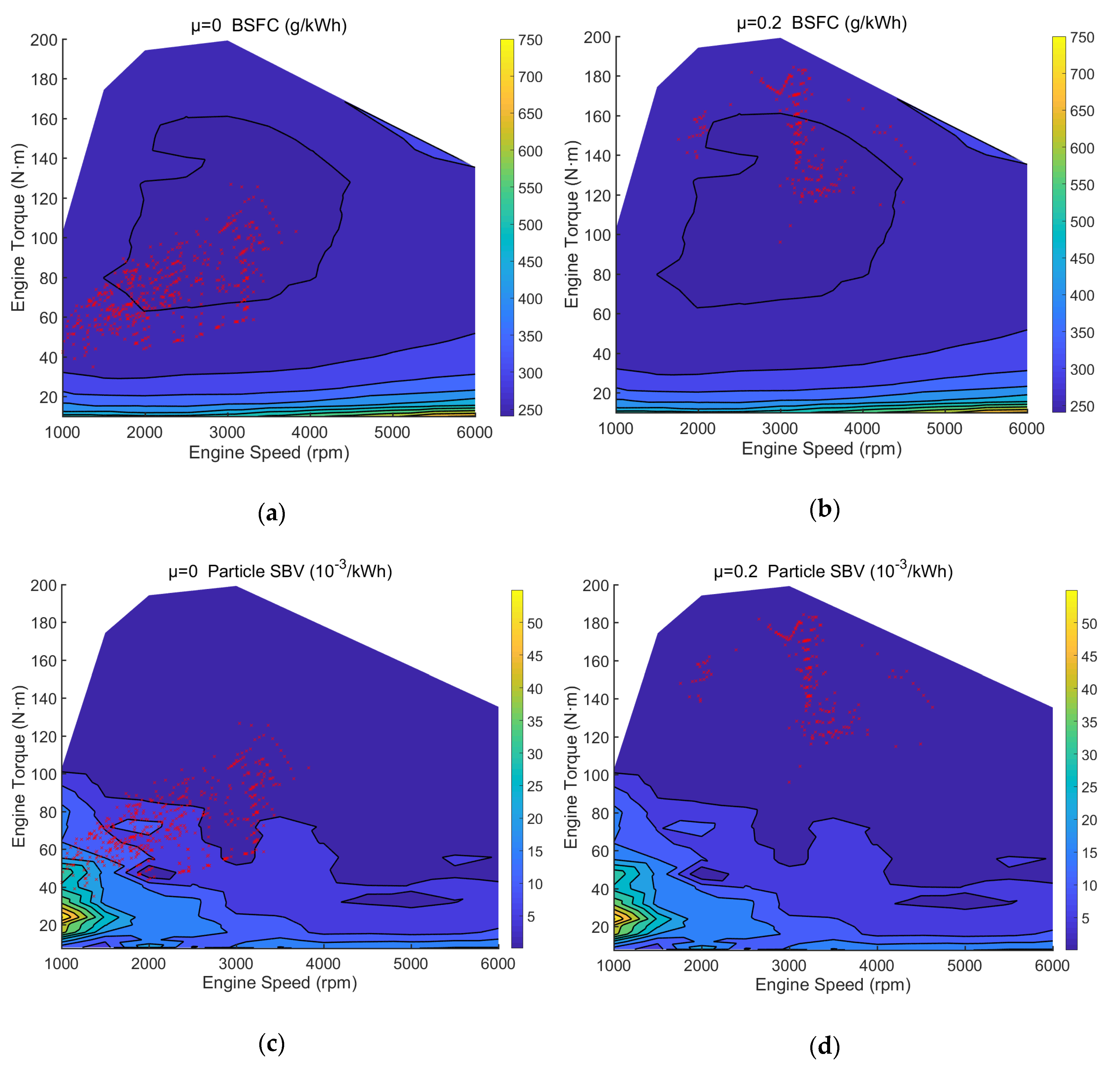
With respect to different weighting coefficients, the simulation results of ${\mu }_{min}$ are presented in Figure 11a,c, contrasted with those of ${\mu }_{max}$ in Figure 11b,d. As shown in Table 3, the cycle time of WLTP is 1800 s. It should be noted that the time step in the MATLAB/SIMULINK model is set as 1 s, which indicates that all operation condition points of the complete WLTP cycle amount to 1800. Red cross dots in Figure 11 represents these operating points.

Applying Equation (10), it is clear that the leverage of emission performance will be not taken into consideration in the ${\mu }_{min}$ scenario. Comparing Figure 11a,b, it can be concluded that the distribution status of brake specific fuel consumption (BSFC) values of all operating points fails to change significantly with $\mu$ increasing from 0 to 0.2. In the ${\mu }_{min}$ scenario where the established objective function only pays attention to energy consumption, nearly half of all operating points are located in the optimal fuel economy area while the other half are mainly located at its periphery area as shown in Figure 11a. By contrast, the above situation seems to stay the same in the ${\mu }_{max}$ scenario where emission performance influence plays an important role as exhibited in Figure 11b, which implies that the overall fuel consumption of these two scenarios are roughly equivalent.

Nevertheless, remarkable differences can be observed when it comes to the amount of particle represented by specific blackening values between these two scenarios. As shown in Figure 11d, operating points are more concentrated in the low SBV area with emission performance assigned with a higher weight in the process of constructing objective function in Equation (10). Comparatively, the distribution status of the ${\mu }_{min}$ scenario appears not as good as the other one. As shown in Figure 11c, quite a few operating points situate in the high SBV area, which means more particle emissions during the whole WLTP test cycle.

Figure 12 and Figure 13 show the variation curves of crucial state parameters including $\mathrm{SOC}$, engine torque, motor torque, and gear of ${\mu }_{min}$ and ${\mu }_{max}$ scenarios, respectively. Associated with the velocity profile of WLTP presented in Figure 10, comparative analysis leads to the conclusion that the engine generally runs in the relatively high-torque region in the ${\mu }_{max}$ scenario. Simultaneously, the frequency of recharging and discharging of the vehicle battery, which is represented by the degree of fluctuation observed in the $\mathrm{SOC}$ or motor torque variation curves, is slightly higher. Conversely, the frequency of the gear shift is strikingly lower than that of the ${\mu }_{min}$ scenario; the corresponding control algorithm will provide the driver with a relatively simple gear shift strategy during the whole WLTP test cycle under the circumstance of the preset value ${\mu }_{max}$. Obviously, relevant adjustment of gear shift strategy makes contribution to the driving experience improvements for the driver.

Figure 14 displays the variation curves of $\mathrm{SOC}$ during the whole WLTP test cycle pertaining to different $\mu$ for emission particles. It can be observed that the maximum decreasing amplitude of $\mathrm{SOC}$ grows larger with $\mu$ gradually increasing. Considering that the higher $\mu$ is, the more attention will be paid to the optimization of emission indicators. As a consequence, the operation range of engine is supposed to be obliged to “comparatively low emissions area” (i.e., the darker areas in Figure 4b) in pursuit of the fulfillment of emission performance considerations. Comparison results in Figure 14 provide solid evidence that motor will make greater contribution to overall power output to compensate the underpowered engine. It is in perfect accordance with the relevant facts demonstrated by the motor variation curves shown in Figure 12 and Figure 13 that motor will act more as a role of power output instead of power generation under the higher $\mu$ circumstance. Meanwhile, it is confirmed again that the preset constraint condition ${\mathrm{SOC}}_0$ must equal ${\mathrm{SOC}}_{\mathrm{final}}$ and further, that is strictly satisfied under different $\mu$ circumstances.

In terms of corresponding simulation results for the other pollutant NOx, similar conclusions can be reached through the same analysis. Due to space limitation, detailed result figures of NOx are presented in Appendix A.

Combining all the simulation results of the series of discrete values $\mu$ for both particle and NOx, Figure 15 exhibits the relationship between emission performance and fuel consumption (FC) based on the 20 obtained sets of data; specific values are listed in

Table A1. The combination of simulation results of the series of discrete values $\mu$.

$\mathit{\mu }$	Particle		NOx
	FC (L/100km)	SBV(-)	FC (L/100km)	Emissions (g)
0.00	3.908	54.92	3.897	28.63
0.01	3.938	44.48	3.903	28.34
0.02	3.992	30.94	3.905	28.16
0.03	4.032	25.57	3.922	27.32
0.04	4.073	19.21	3.928	27.10
0.05	4.116	14.76	3.931	26.78
0.06	4.153	13.93	3.935	26.43
0.07	4.172	13.84	3.939	26.16
0.08	4.181	13.82	3.950	25.74
0.09	4.197	13.84	3.962	25.04
0.10	4.221	13.79	3.995	23.63
0.11	4.246	13.82	4.007	23.42
0.12	4.278	12.80	4.012	23.32
0.13	4.293	11.93	4.033	23.15
0.14	4.324	11.56	4.045	22.96
0.15	4.348	11.32	4.052	22.90
0.16	4.377	10.92	4.068	22.85
0.17	4.391	10.51	4.075	22.81
0.18	4.418	10.29	4.083	22.78
0.19	4.439	9.90	4.096	22.76
0.20	4.466	9.63	4.105	22.75

in Appendix A. The data points of particle are marked as 20 red plus dots; those of NOx are marked as blue cross dots. Considering the complete WLTP test cycle, the calculation results of each time step add up to the integrated FC in L/100km and total emissions (i.e., NOx emissions in grams and particle emissions in SBV). As shown in Figure 15, data points located from top left to bottom right signify the simulation results of increasing $\mu$ for both exhaust pollutants. By analysis of the curve trend, it is clear that there exists a trade-off relationship between fuel economy and emission performance, whether it is for NOx or particle. As the weighting coefficient $\mu$ grows up, relevant results indicating worse fuel economy and better emission performance simultaneously are attained through simulation, which also conforms to a previous inference derived from $J_{MP}\left(t\right)$, set up in Equation (15).

Considering that the investigated P3 HEV is oriented at Europe and China auto market, both the latest European emission standard (i.e., Euro 6c) and the Chinese counterpart (i.e., China VI) are investigated and the emission limits of particle and NOx are shown in

Table 5. Comparison between simulation results and the latest emission standards.

Scenarios	Particle Emissions (Nb/km)	NOx Emissions (mg/km)
${\mu }_{min}=0.00$	$3.0\times {10}^{12}$	1231
${\mu }_{max}=0.20$	$5.0\times {10}^{11}$	978
China VI	$6.0\times {10}^{11}$	60
Euro 6c	$6.0\times {10}^{11}$	75

[43,44,45,46,47]. Moreover, the simulation results obtained from the two most representative scenarios (i.e., ${\mu }_{min}=0.00$ and ${\mu }_{max}=0.20$) are also presented in Table 5 as a contrast. It should be noted that the unit of particle emissions used in China VI and Euro 6c is the number (Nb) of particle per kilometer rather than SBV employed in this paper. Therefore, the conversion of the relevant numerical values is supposed to be performed beforehand. In terms of particle emissions, it can be concluded that the particle number (PN) is more than five times the limit of China VI/Euro 6c in the ${\mu }_{min}$ scenario where the established objective function only pays attention to energy consumption. Conversely, the PN succeeds in meeting the requirements of these two emission legislations in the ${\mu }_{max}$ scenario where the emission performance indicator is endowed with a substantial weight. An obvious conclusion that can be drawn is that the effectiveness of the proposed control algorithm is validated once again. With respect to NOx emissions, it is clear that ${\mu }_{min}$ or ${\mu }_{max}$ scenario yields results that significantly exceed the limits of the China VI/Euro 6c. As mentioned above, the experimental data of NOx emission is directly captured from the exhaust pipe located before the catalytic converter, which causes its numerical values considerable, thus the optimization effect will be heightened. Actually, HEVs are supposed to be equipped with catalytic converters in order to fulfil the relevant NOx limitations of the China VI/Euro 6c in the real world.

4.3. Comparison between DP and ECMS

Actual execution time features prominently in the practicability of proposed algorithm. In the real world, classical DP algorithm is subject to online application restrictions in most cases because of prohibitive time expenditure. Nevertheless, a real sense of global optimal solution can be obtained by DP algorithm. In contrast to DP, solutions found by ECMS or other simplification algorithm generally suffer, to some extent, local optimal traps. Consequently, offline calculation results based on DP are commonly set as a reference for comparison [48,49,50].

As mentioned above, the proposed control algorithm design is developed on the basis of ECMS. Instead of applying quadratic polynomial fitting method for the sake of the simplification of objective function, the classical DP algorithm employs a comparatively straightforward traversal method in order to identify the specific location of the optimal point. During the optimization process of searching the minimal value of $J_{MP}\left(t\right)$, the DP algorithm basically calculates the specific values of $J_{MP}\left(t\right)$ under all possible operation conditions and sorts out the corresponding output torque configurations (i.e., $M_{op}$) for $J_{MP}{\left(t\right)}_{min}$. It should be noted that the detailed numerical calculation in the DP algorithm is predicated on the raw experimental data (e.g., the emissions map of two main pollutants particle and NOx as shown in Figure 4) rather than fitting results, which on the one hand guarantees the precision of the global optimal solution obtained by DP algorithm, but on the other hand makes it significantly time-consuming.

Considering both exhaust pollutants, Figure 16 displays the comparison between simulation results of DP and ECMS; the specific relative error (RE) data are presented in

Table A2. The relative error between simulation results of DP and ECMS.

$\mathit{\mu }$	Particle		NOx
	FC RE (%)	SBV RE (%)	FC RE (%)	Emissions RE (%)
0.00	0.252	0.019	0.256	0.045
0.01	0.217	0.031	0.334	0.036
0.02	0.206	0.089	0.367	0.017
0.03	0.36	0.017	0.247	0.034
0.04	0.367	0.038	0.214	0.014
0.05	0.254	0.063	0.342	0.033
0.06	0.369	0.044	0.271	0.011
0.07	0.284	0.031	0.318	0.012
0.08	0.282	0.045	0.237	0.039
0.09	0.218	0.022	0.249	0.061
0.10	0.288	0.048	0.368	0.042
0.11	0.304	0.019	0.228	0.043
0.12	0.249	0.094	0.202	0.054
0.13	0.235	0.118	0.296	0.056
0.14	0.275	0.121	0.221	0.017
0.15	0.305	0.131	0.28	0.044
0.16	0.339	0.083	0.364	0.092
0.17	0.258	0.076	0.355	0.043
0.18	0.316	0.092	0.313	0.014
0.19	0.354	0.023	0.245	0.043

in Appendix A. It can be concluded from Figure 16 that DP yields global optimal data points distinguishing from those local optimal counterparts of ECMS with only slightly perceptible difference, which thus demonstrates the accuracy and feasibility of the proposed control algorithm predicated on ECMS.

5. Discussions and Conclusions

Continuous deterioration of the global atmospheric environment has given rise to the prosperity of so-called green vehicles. Therefore, HEVs have drawn extensive attention from academia and the automobile industry alike as a practicable technical route. With respect to the EMS design, which undoubtedly occupies an indispensable position in HEVs advance, strategic planning are in particular required in order to boost the overall performance improvement of the HEV powertrain. In consideration of tightening regulations on vehicle exhausts, it seems natural that there needs to be more concern about vehicle emission performance during the design process of the control algorithm design for the EMS in HEV powertrain.

However, few previous studies have deeply investigated a feasible control algorithm, simultaneously considering both energy consumption and emission performance. To illuminate the uncharted area, we present a novel design scheme incorporating the aforementioned two performance evaluation indicators into a single objective function based on ECMS. Massive bench test data have been collected as the prerequisite for subsequent modeling. Quadratic polynomial fitting method is appropriately applied into the process of determining the specific values of corresponding indicators. This operation not only guarantees that both consumed power and specific emission rate can be incorporated into an integral objective function because of their parallel structures of mathematical expressions, but it also significantly improves the computation speed of the proposed control algorithm because the identification process of the optimal point can be performed accurately and promptly.

Subsequently, a comprehensive multi-parameter objective function is established on the grounds of ECMS with the relevant simulation models constructed in MATLAB/SIMULINK. The proposed control algorithm design is validated against the simulation results predicated on WLTP. The impacts of weighting coefficients pertaining to two exhaust pollutants upon the specific configurations of the proposed control algorithm are discussed in detail. Furthermore, comparative analysis of the simulation results obtained from ECMS and classical DP algorithm, respectively, is performed. In the present study, we mainly focus on the algorithm structure design and preliminary simulation verification. Further, we think that the present research findings may not be optimal but should be sufficient to provide requisite guidance necessary for the appropriate design of control algorithm for EMS, which undoubtedly plays a vital role in the HEV powertrain performance improvement. Although demonstrated by preliminary simulation results, this proposed control algorithm design suffers from some limitations due to the lack of real road running experimental data from the vehicle equipped with the redesigned EMS. However, the obtained results can still cast a new light on the control algorithm design for EMS in HEV powertrain despite that inadequacy. Detailed analysis leads to the following conclusions:

• The indicators of both energy consumption and emission performance are accurately modeled by applying the quadratic polynomial fitting method. Fitting results of corresponding relation curves show good agreement with the raw data obtained from bench test, which lays a solid foundation for subsequently incorporating the aforementioned considerations into the integrated objective function.
• With respect to the related mathematical expression of the combined objective function, a three-stage piecewise quadratic function is attained. Furthermore, it is confirmed that the identification of corresponding optimal point can be performed precisely and promptly, which consequently yields significant computation speed advantages when compared with the classical DP algorithm.
• Remarkable changes can be observed in the simulation results between weighting coefficients $\mu$. Under the circumstance of emission performance assigned with a higher weight, findings prove that the operation range of engine is obliged to “comparatively low emissions area” while motor makes greater contribution to the overall power output. Considering the series of discrete values $\mu$, analysis of curve trend demonstrates that there exists a trade-off relationship between fuel economy and emission performance, whether it is for NOx or particle.
• A comparative investigation of the simulation results from ECMS and DP respectively validates the feasibility and accuracy of the proposed control algorithm design predicated on ECMS.

References

1. Stone, R. Introduction to Internal Combustion Engines, 2nd ed.; Palgrave Macmillan: London, UK, 1985; pp. 23–25. ISBN 978-1-349-22147-9. [Google Scholar]
2. Guzzella, L.; Onder, C.H. Introduction to Modeling and Control of Internal Combustion Engine Systems; Springer: Berlin, Germany, 2010; pp. 2622–2626. ISBN 978-3-662-08003-0. [Google Scholar]
3. Taylor, A.M.K.P. Science review of internal combustion engines. Energy Policy 2008, 36, 4657–4667. [Google Scholar] [CrossRef]
4. Qiao, Y.; Huang, K.; Jeub, J.; Qian, J.; Song, Y. Deploying Electric Vehicle Charging Stations Considering Time Cost and Existing Infrastructure. Energies 2018, 11, 2436. [Google Scholar] [CrossRef]
5. Groff, E.G. Automotive Two-Stroke-Cycle Engine Development in the 1980-1990’s; Technical Paper; SAE International: Detroit, MI, USA, 2016. [Google Scholar]
6. Krutilla, K.; Graham, J.D. Are Green Vehicles Worth the Extra Cost? The Case of Diesel-Electric Hybrid Technology for Urban Delivery Vehicles. J. Policy Anal. Manag. 2012, 31, 501–532. [Google Scholar] [CrossRef]
7. Wang, F.K.; Saito, M. Evaluating the efficiency of green vehicles and diesel vehicles. Int. J. Green Energy 2016, 13, 1163–1174. [Google Scholar] [CrossRef]
8. Haddadian, G.; Khodayar, M.; Shahidehpour, M. Accelerating the global adoption of electric vehicles: Barriers and drivers. Electr. J. 2015, 28, 53–68. [Google Scholar] [CrossRef]
9. Trigg, T.; Telleen, P.; Boyd, R.; Cuenot, F.; D’Ambrosio, D.; Gaghen, R.; Gagné, J.; Hardcastle, A.; Houssin, D.; Jones, A. Global EV outlook: Understanding the electric vehicle landscape to 2020. Int. Energy Agency 2013, 1, 1–40. [Google Scholar]
10. Reddi, K.; Elgowainy, A.; Rustagi, N.; Gupta, E. Impact of hydrogen refueling configurations and market parameters on the refueling cost of hydrogen. Int. J. Hydrog. Energy 2017, 42, 21855–21865. [Google Scholar] [CrossRef]
11. Enang, W.; Bannister, C. Modelling and control of hybrid electric vehicles (A comprehensive review). Renew. Sustain. Energy Rev. 2017, 74, 1210–1239. [Google Scholar] [CrossRef] [Green Version]
12. Geetha, A.; Subramani, C. A comprehensive review on energy management strategies of hybrid energy storage system for electric vehicles. Int. J. Energy Res. 2017, 41, 1817–1834. [Google Scholar] [CrossRef]
13. Tie, S.F.; Tan, C.W. A review of energy sources and energy management system in electric vehicles. Renew. Sustain. Energy Rev. 2013, 20, 82–102. [Google Scholar] [CrossRef]
14. Lim, D.J.; Jahromi, S.R.; Anderson, T.R.; Tudorie, A.A. Comparing technological advancement of hybrid electric vehicles (HEV) in different market segments. Technol. Forecast. Soc. Chang. 2015, 97, 140–153. [Google Scholar] [CrossRef] [Green Version]
15. Homchaudhuri, B.; Lin, R.; Pisu, P. Hierarchical control strategies for energy management of connected hybrid electric vehicles in urban roads. Transp. Res. Part C Emerg. Technol. 2016, 62, 70–86. [Google Scholar] [CrossRef] [Green Version]
16. Zhang, P.; Yan, F.; Du, C. A comprehensive analysis of energy management strategies for hybrid electric vehicles based on bibliometrics. Renew. Sustain. Energy Rev. 2015, 48, 88–104. [Google Scholar] [CrossRef]
17. Bayindir, K.Ç.; Gözüküçük, M.A.; Teke, A. A comprehensive overview of hybrid electric vehicle: Powertrain configurations, powertrain control techniques and electronic control units. Energy Convers. Manag. 2011, 52, 1305–1313. [Google Scholar] [CrossRef]
18. Yi, C.; Epureanu, B.I.; Hong, S.K.; Ge, T.; Yang, X.G. Modeling, control, and performance of a novel architecture of hybrid electric powertrain system. Appl. Energy 2016, 178, 454–467. [Google Scholar] [CrossRef]
19. Shabbir, W.; Evangelou, S.A. Real-time control strategy to maximize hybrid electric vehicle powertrain efficiency. Appl. Energy 2014, 135, 512–522. [Google Scholar] [CrossRef]
20. Sockeel, N.; Shi, J.; Shahverdi, M.; Mazzola, M. Pareto Front Analysis of the Objective Function in Model Predictive Control Based Power Management System of a Plug-in Hybrid Electric Vehicle. In Proceedings of the 2018 IEEE Transportation Electrification Conference and Expo (ITEC), Chicago, IL, USA, 13–15 June 2018; pp. 1–6. [Google Scholar]
21. Sockeel, N.; Shahverdi, M.; Mazzola, M. Impact of the State of Charge estimation on Model Predictive Control Performance in a Plug-in Hybrid Electric Vehicle accounting for equivalent fuel consumption and battery capacity fades. In Proceedings of the 2019 IEEE Transportation Electrification Conference and Expo (ITEC), Detroit, MI, USA, 19–21 June 2019; pp. 127–136. [Google Scholar]
22. Huang, Y.; Wang, H.; Khajepour, A.; He, H.; Ji, J. Model predictive control power management strategies for HEVs: A review. J. Power Sources 2017, 341, 91–106. [Google Scholar] [CrossRef]
23. Di Cairano, S.; Bernardini, D.; Bemporad, A.; Kolmanovsky, I.V. Stochastic MPC with learning for driver-predictive vehicle control and its application to HEV energy management. IEEE Trans. Control Syst. Technol. 2013, 22, 1018–1031. [Google Scholar] [CrossRef]
24. Yan, F.; Wang, J.; Huang, K. Hybrid electric vehicle model predictive control torque-split strategy incorporating engine transient characteristics. IEEE trans. Veh. Technol. 2012, 61, 2458–2467. [Google Scholar] [CrossRef]
25. Minh, V.; Rashid, A. Modeling and model predictive control for hybrid electric vehicles. Int. J. Automot. Technol. 2012, 13, 477–485. [Google Scholar] [CrossRef]
26. Xiang, C.; Ding, F.; Wang, W.; He, W. Energy management of a dual-mode power-split hybrid electric vehicle based on velocity prediction and nonlinear model predictive control. Appl. Energy 2017, 189, 640–653. [Google Scholar] [CrossRef]
27. Ibrahim, M.; Jemei, S.; Wimmer, G.; Hissel, D. Nonlinear autoregressive neural network in an energy management strategy for battery/ultra-capacitor hybrid electrical vehicles. Electr. Power Syst. Res. 2016, 136, 262–269. [Google Scholar] [CrossRef]
28. Paganelli, G.; Delprat, S.; Guerra, T.M.; Rimaux, J.; Santin, J.J. Equivalent consumption minimization strategy for parallel hybrid powertrains. In Proceedings of the 2002 IEEE Vehicular Technology Conference, Birmingham, AL, USA, 6–9 May 2002; pp. 2076–2081. [Google Scholar]
29. Onori, S.; Serrao, L.; Rizzoni, G. Hybrid Electric Vehicles Energy Management Strategies; Springer: London, UK, 2016; pp. 65–77. ISBN 978-1-4471-6781-5. [Google Scholar]
30. Teng, L.; Hu, X.; Li, S.E.; Cao, D. Reinforcement Learning Optimized Look-Ahead Energy Management of a Parallel Hybrid Electric Vehicle. IEEE/ASME Trans. Mechatron. 2017, 22, 1497–1507. [Google Scholar]
31. Alegre, S.; Míguez, J.V.; Carpio, J. Modelling of electric and parallel-hybrid electric vehicle using Matlab/Simulink environment and planning of charging stations through a geographic information system and genetic algorithms. Renew. Sustain. Energy Rev. 2017, 74, 1020–1027. [Google Scholar] [CrossRef]
32. Barth, M.; An, F.; Norbeck, J.; Ross, M. Modal emissions modeling: A physical approach. Transp. Res. Rec. 1996, 1520, 81–88. [Google Scholar] [CrossRef]
33. Cappiello, A.; Chabini, I.; Nam, E.K.; Lue, A.; Zeid, M.A. A statistical model of vehicle emissions and fuel consumption. In Proceedings of the 2002 IEEE 5th International Conference on Intelligent Transportation Systems, Singapore, 3–6 September 2002; pp. 801–809. [Google Scholar]
34. Ahn, K.; Rakha, H.; Trani, A.; Van Aerde, M. Estimating vehicle fuel consumption and emissions based on instantaneous speed and acceleration levels. J. Transp. Eng. 2002, 128, 182–190. [Google Scholar] [CrossRef]
35. Rakha, H.; Ahn, K.; Trani, A. Development of VT-Micro model for estimating hot stabilized light duty vehicle and truck emissions. Transp. Res. Part D: Transp. Environ. 2004, 9, 49–74. [Google Scholar] [CrossRef]
36. Asher, Z.; Galang, A.; Briggs, W.; Johnston, B. Economic and Efficient Hybrid Vehicle Fuel Economy and Emissions Modeling Using an Artificial Neural Network; Technical Paper; SAE International: Detroit, MI, USA, 2018. [Google Scholar]
37. Qiao, Y.; Duan, X.; Huang, K.; Song, Y.; Qian, J. Scavenging Ports’ Optimal Design of a Two-Stroke Small Aeroengine Based on the Benson/Bradham Model. Energies 2018, 11, 2739. [Google Scholar] [CrossRef]
38. Serrao, L.; Onori, S.; Rizzoni, G. ECMS as a realization of Pontryagin’s minimum principle for HEV control. In Proceedings of the 2009 IEEE American Control Conference, St. Louis, MO, USA, 10–12 June 2009; pp. 3964–3969. [Google Scholar]
39. Demuynck, J.; Bosteels, D.; De Paepe, M.; Favre, C.; May, J.; Verhelst, S. Recommendations for the new WLTP cycle based on an analysis of vehicle emission measurements on NEDC and CADC. Energy Policy 2012, 49, 234–242. [Google Scholar] [CrossRef] [Green Version]
40. Pavlovic, J.; Marotta, A.; Ciuffo, B. CO2 emissions and energy demands of vehicles tested under the NEDC and the new WLTP type approval test procedures. Appl. Energy 2016, 177, 661–670. [Google Scholar] [CrossRef]
41. Pavlovic, J.; Ciuffo, B.; Fontaras, G.; Valverde, V.; Marotta, A. How much difference in type-approval CO2 emissions from passenger cars in Europe can be expected from changing to the new test procedure (NEDC vs. WLTP)? Transp. Res. Part A Policy Pract. 2018, 111, 136–147. [Google Scholar] [CrossRef]
42. Fontaras, G.; Ciuffo, B.; Zacharof, N.; Tsiakmakis, S.; Marotta, A.; Pavlovic, J.; Anagnostopoulos, K. The difference between reported and real-world CO2 emissions: How much improvement can be expected by WLTP introduction? Transp. Res. Procedia 2017, 25, 3933–3943. [Google Scholar] [CrossRef]
43. Ciuffo, B.; Maratta, A.; Tutuianu, M.; Anagnostopoulos, K.; Fontaras, G.; Pavlovic, J.; Serra, S.; Tsiakmakis, S.; Zacharof, N. Development of the Worldwide Harmonized Test Procedure for Light-Duty Vehicles: Pathway for Implementation in European Union Legislation. Transp. Res. Rec. 2015, 2503, 110–118. [Google Scholar] [CrossRef]
44. Mera, Z.; Fonseca, N.; López, J.M.; Casanova, J. Analysis of the high instantaneous NOx emissions from Euro 6 diesel passenger cars under real driving conditions. Appl. Energy 2019, 242, 1074–1089. [Google Scholar] [CrossRef]
45. Suarez-Bertoa, R.; Astorga, C. Impact of cold temperature on Euro 6 passenger car emissions. Environ. Pollut. 2018, 234, 318–329. [Google Scholar] [CrossRef] [PubMed]
46. Zhang, S.; Wu, Y.; Wu, X.; Li, M.; Ge, Y.; Liang, B.; Xu, Y.; Zhou, Y.; Liu, H.; Fu, L. Historic and future trends of vehicle emissions in Beijing, 1998–2020: A policy assessment for the most stringent vehicle emission control program in China. Atmos. Environ. 2014, 89, 216–229. [Google Scholar] [CrossRef]
47. Wu, X.; Wu, Y.; Zhang, S.; Liu, H.; Fu, L.; Hao, J. Assessment of vehicle emission programs in China during 1998–2013: Achievement, challenges and implications. Environ. Pollut. 2016, 214, 556–567. [Google Scholar] [CrossRef] [PubMed]
48. Wahl, H.G.; Gauterin, F. An Iterative Dynamic Programming Approach for the Global Optimal Control of Hybrid Electric Vehicles under Real-time Constraints. In Proceedings of the 2013 IEEE Intelligent Vehicles Symposium, Gold Coast City, Australia, 23–26 June 2013; pp. 592–597. [Google Scholar]
49. Lian, H.; Zeng, C.; Cai, Z. Dynamic programming based optimal control strategy of the hybrid vehicular power system. In Proceedings of the 2017 43rd Annual Conference of the IEEE Industrial Electronics Society, Beijing, China, 29 October–1 November 2017; pp. 7123–7127. [Google Scholar]
50. Ozatay, E.; Onori, S.; Wollaeger, J.; Ozguner, U.; Rizzoni, G.; Filev, D.; Michelini, J.; Cairano, S.D. Cloud-Based Velocity Profile Optimization for Everyday Driving: A Dynamic-Programming-Based Solution. IEEE Trans. Intell. Transp. Syst. 2014, 15, 2491–2505. [Google Scholar] [CrossRef]
Figure 1. Structure of the investigated P3 hybrid electric vehicles (HEV) powertrain.
Energies 12 02698 g001
Figure 2. Fitting results of the chemical energy consumed power.
Energies 12 02698 g002
Figure 3. Fitting results of the electric energy consumed power.
Energies 12 02698 g003
Figure 4. Emissions map of two main pollutants: (a) NOx and (b) Particle.
Energies 12 02698 g004
Figure 5. Quadratic polynomial fitting results of two main pollutants: (a) NOx and (b) Particle.
Energies 12 02698 g005
Figure 6. The optimal point identification for one scenario.
Energies 12 02698 g006
Figure 7. All possible scenarios of the piecewise quadratic function.
Energies 12 02698 g007
Figure 8. Unified modeling language (UML) activity diagram for the control algorithm.
Energies 12 02698 g008
Figure 9. The velocity profile of the New European Driving Cycle (NEDC).
Energies 12 02698 g009
Figure 10. The velocity profile of the Worldwide-Harmonized Light-Vehicle Test Procedure (WLTP).
Energies 12 02698 g010
Figure 11. Comparison results of different weighting coefficients for emission particle. (a) μ = 0 BSFC; (b) μ = 0.2 BSFC; (c) μ = 0 Particle SBV; (d) μ = 0.2 Particle SBV.
Energies 12 02698 g011
Figure 12. Three state parameters’ variation curves of μ m i n for emission particle.
Energies 12 02698 g012
Figure 13. Three state parameters’ variation curves of μ m a x for emission particle.
Energies 12 02698 g013
Figure 14. The variation curves of SOC pertaining to different μ for emission particle.
Energies 12 02698 g014
Figure 15. The combination of simulation results of the series of discrete values μ .
Energies 12 02698 g015
Figure 16. The comparison between simulation results of Dynamic Programming (DP) and Equivalent Consumption Minimization Strategy (ECMS): (a) Particle and (b) NOx.
Energies 12 02698 g016