Article

Optimising the Operation of Tidal Range Schemes

Cardiff School of Engineering, Cardiff University, Cardiff CF24 3AA, UK
*
Author to whom correspondence should be addressed.
Energies 2019, 12(15), 2870; https://doi.org/10.3390/en12152870
Submission received: 3 July 2019 / Revised: 19 July 2019 / Accepted: 23 July 2019 / Published: 25 July 2019
(This article belongs to the Section A3: Wind, Wave and Tidal Energy)

Abstract

:
Marine renewable energy, including tidal renewable energy, is one of the less exploited sources of energy that could contribute to energy demand, while reducing greenhouse gas emissions. Amongst several proposals to build tidal range structure (TRS), a tidal lagoon has been proposed for construction in Swansea Bay, in the South West of the UK, but this scheme was recently rejected by the UK government due to the high electricity costs. This decision makes the optimisation of such schemes more important for the future. This study proposes various novel approaches by breaking the operation into small components to optimise the operation of TRS using a widely used 0-D modelling methodology. The approach results in a minimum 10% increase in energy output, without the inclusion of pumping, in comparison to the maximum energy output using a similar operation for all tides. This increase in energy will be approximately 25% more when pumping is included. The optimised operation schemes are used to simulate the lagoon operation using a 2-D model and the differences between the results are highlighted.

Graphical Abstract

1. Introduction

With improvements in environmental awareness globally, emission levels of CO2 are expected to decrease by reducing reliance on fossil fuels, and further development in renewable energy. The UK government aims to produce 15% of its total energy from renewable resources by 2020, which corresponds to approximately 35% of the UK’s electricity demand [1,2,3]. Marine renewable energy (MRE) is one of the emerging renewable energies being explored further. Currently, 0.5 GWh of commercial marine energy generation capacity is in operation and another 1.7 GWh is under construction, with most of this accounted for tidal range [4].
It has been suggested that the tidal range resources of the UK is able to deliver 25 GW theoretically [5]. A number of TRS have been proposed around the UK, particularly in the Severn Estuary and Bristol Channel, with these estuaries being located in the South West of the UK, as shown in Figure 1. Swansea Bay Lagoon is one of these projects, which has been one of the world’s first tidal lagoon power plants [6]. It was granted planning permission by the UK Department of Energy and Climate Change (DECC) in June 2015 [7] and was positively supported by the independent Hendry Review of tidal lagoons, commissioned by the UK government and published in January 2017 [8]. However, the cost of electricity has been found to be an issue [9] and the UK government Business and Energy Secretary Greg Clark said that the £1.3bn project was not good value for money, despite claims to the contrary by the developers Tidal Lagoon Power [10]. There have been different values reported for the cost of electricity. The general figure quoted for the levelised cost of electricity (LCOE) is reported to be £150/MWh [11], while the consumer cost over the lifetime of the project is reported to be £25.78/MWh [12]. This reemphasises the need for further optimisation of tidal range structures to enable such projects to produce competitive energy costs.
Tidal range structure (TRS) creates an artificial head difference across the scheme and generates energy using this head difference. The schemes could be operated to generate energy during flood tide (flood generation), ebb tide (ebb generation), and on both ebb and flood tides (two-way generation). One of the key aspects of the operation of such schemes is the head difference at the time when the scheme would be programmed to start generating energy and when generation stops (further details on the operation of TRS is provided in Section 2). Therefore, TRS can be operated in various ways for each type of operation scheme, i.e., for flood, ebb, or two-way generation, and this operation will influence the basin water level and discharge transferred between the impoundment and open waters, and therefore affecting the energy generated. 0-D models have been widely used in designing TRS and particularly in initially optimising the operation of such schemes [13,14,15,16]. Fundamental theoretical research was carried out in this field by Prandle in the 1980s [17]. Eight dimensionless parameters were defined to provide a formulation for the design characteristics and energy calculations, using four key assumptions that affect the energy predictions. For example, the energy generation starts and stops at the same prescribed minimum head, i.e., ηmin, which can affect the energy output significantly. Aggidis and Benzon used a 0-D model to evaluate the energy (electricity) generation in relation to varying trends in energy demand [13]. They optimised driving heads based on the size and number of turbines, which varies with the barrage and/or lagoon dimensions and characteristics. These studies have demonstrated that the 0-D approach has significant preliminary design potential for all types of tidal impoundments.
However, Angeloudis et al. showed that 0-D models can overestimate the energy predictions by up to 40% when compared to prediction based on more sophisticated and accurate 2-D numerical models [18,19]. They concluded that the 0-D approach overestimation is relative to the size of the scheme. They suggested that 0-D predictions are only reliable for design optimisation at the preliminary stage and need to be complemented by more sophisticated 2-D models. It should be noted that all three studies have used constant driving and minimum generation heads throughout the operation, i.e., for all spring and neap and flood and ebb tides. Based on the authors’ extensive literature review, Ahmadian et al. [15] and Yates et al. [14] have separately discussed the concept of variable driving and minimum generation heads for each operation period, namely half a tide, and highlighted the potential improvements achievable by implementing variable driving and minimum generation heads. More recently, Angeloudis et al. also took advantage of a gradient-based method for the optimisation of flexible operation heads [16].
Research on using pumping to increase energy generation has been limited and was mainly carried out using a constant driving and minimum generation head throughout. Yates et al. used an unlimited pumping head and constant generating head to study the influence of turbining and pumping efficiencies in a 0-D model [20]. They found that the overall energy could improve by about 17% if pumping was included in a two-way generation scheme using constant values for turbine and pump efficiencies. Furthermore, Douglas et al. showed that pumping could increase energy generation by approximately 10% [21]. Their results were consistent with the findings of Aggidis and Benzon [13]. However, they used the same hill-chart for both the energy generation and pumping phases, with a scaled down maximum energy output. With lack of detailed information, they also assumed a combined efficiency during the pumping phase. In the literature, there are a very limited number of studies for the case of pumping, with the majority of studies using a constant pumping head and constant starting and ending head difference for the schemes, with virtually no research being undertaken into measuring the pumping efficiency. Consequently, adding flexible operating heads for the whole tidal cycle, including pumping with flexible operating heads, is another novel aspect being investigated in this study.
This paper focuses on facilitating the development of TRS by using a novel approach that includes splitting the operation for each tidal cycle up into smaller components and optimising the operation of TRS, in order to generate the maximum energy and therefore reduce the cost of the energy generation. Flexible operation was implemented with variable operational heads and optimised using various combination of tides and utilising a 0-D model. The optimised outcomes were further improved by considering pumping with more optimised operational characteristics in order to increase energy generation. The results were then compared using a more sophisticated 2-D unstructured grid model, namely the depth integrated velocities and solute transport (DIVAST 2-DU) model, with the differences between energy output and performance being highlighted from the predictions obtained for the 0-D and 2-D models.

2. Tidal Range Schemes

2.1. No-Pumping Operation

Xia et al. [22] showed that the two most effective operational schemes are ebb-only and two-way generation. Therefore, this study mainly focuses on these operational schemes, and schematic illustrations of them are shown in Figure 2a,b, respectively.
Starting at a high tide, ebb-only generation starts with a holding stage where both the turbines and sluice gates are closed and there is no flow between the outside sea and the impounded water body. Therefore, the impounded basin water level stays at around high tide, while the seaward water level recedes with the tide. Ebb generation phase commences when the head difference between the water level inside and outside the basin, referred to as Hse herein, is large enough to generate energy efficiently through opening only the turbines. This ebb generation phase then continues until the head difference across the impoundment embankment is not sufficient to generate energy efficiently, referred to as Hee herein. At this time, the second holding phase commences, with both the turbines and sluice gates being closed. The downstream water levels are then raised again with the flooding tide and the filling phase starts by opening both sluice gates and turbines (without generating energy) when the seaward water levels are higher than the water level inside the basin. This filling stage is followed by a holding phase for the next cycle when the water levels reach almost the same level, both inside and outside of the impoundment close to high tide. A schematic of the ebb generation scheme is illustrated in Figure 2a.
For two-way generation and starting from the ebb holding phase, where both the sluice gates and turbines are closed, the holding phase continues until the head difference across the impoundment embankment is large enough for efficient generation, in other words, reaching a starting head for ebb tides of Hse. This stage of the ebb generating phase starts by operating the turbines in order to generate energy and continues until the head difference across the impoundment is no longer adequate for efficient energy generation, i.e., reaching the ending head Hee towards the end of ebb tide. Near the end of ebb tide, the sluice gates are opened to empty the basin, until the water levels across the impoundment embankment are almost the same. Following this step, the flood-holding phase begins by closing the turbines and sluice gates until the head difference is higher than the starting head during flooding, i.e., Hsf. This is followed by the flood generation phase, where the turbines are operated again to generate energy. When the head difference is smaller than ending head, namely Hef, the sluice gates are again opened to raise the water levels inside the impoundment. The filling phase now stops and the ebb holding phase starts again, when the water levels across the impoundment embankment reach the same levels and the water level outside the impoundment starts falling again with the ebbing tide falling again with the ebbing tide. This can be seen as a periodic process, which repeats itself throughout each cycle. A schematic of the two-way generation scheme is illustrated in Figure 2b.

2.2. Including Pumping

The total energy generated by a tidal range scheme can be potentially increased by taking advantage of pumping, at high and low water. If the turbines are also designed for pumping, there will not be any significant increase in the cost of the scheme. However, pumping could also bring additional environmental benefits [23], as well as generating more energy.
In practise, pumping is introduced during the holding phases. In the ebb-only generation mode, the objective is to raise the water level inside the basin to a maximum by pumping when the water level difference across the impoundment embankment is small. This generates a bigger head difference Hps, and in turn more energy when the seaward water level falls with the ebbing tide. For the two-way generation scheme, pumping during ebb generation will be similar to pumping for the ebb-only scheme. Pumping will be used to lower the water levels Hpe inside the basing during the flood-holding phase. This will generate a higher head difference during the flood generation phase. Pumping is economically feasible when the combined efficiency losses of pumping and generation are offset by the gained energy output as a result of an increased head difference. Schematic illustrations for ebb-only and two-way generation with pumping are illustrated in Figure 3a,b, respectively.

3. Swansea Bay Lagoon

Swansea Bay is located in the South West of the United Kingdom and constitutes part of the South Wales coastline. As a part of the Bristol Channel, the tidal range in the bay often exceeds 10 m [24], which makes it a suitable location for a tidal range scheme. The Swansea Bay Tidal Lagoon was proposed by tidal lagoon power (TLP) in 2004 [25]. The proposed lagoon wall would be 9.5 km long, creating a lagoon area of about 11.5 km2. The scheme would have an energy-generating life of 120 years and would consist of 16 bulb turbines, each of diameter 7.2 m, and with an installed capacity of 320 MW [7]. The area of the sluice gates would be approximately 800 m2 and the lagoon was designed to be operated using the two-way generation [24,25] as outlined above. Based on the most recent report published by TLP [7], the annual energy generated is predicted to be 530 GWh per year.

4. Modelling Methodology

4.1. 0-D Modelling

4.1.1. 0-D Model Setup

A typical 0-D backward difference model was developed to solve the continuity equation. The new upstream water levels inside the impoundment ( Z up , i   +   1 ) at any point in time can be calculated according to both the upstream water levels at the previous time step ( Z up , i ) and the downstream water levels ( Z dn , i ), as follows:
Z up , i   +   1 = Z up , i + Q ( H ) + Q in A Δ t
where Δ t denotes the time step; Q in is the inflow/outflow to the lagoon through sources other than through the TRS, e.g., a river or outflows; A is the wetted plan surface area of the lagoon and Q ( H ) is the total discharge through the turbines and sluices and which will be discussed further in Section 4.1.2 [19].
In the absence of substantial wetting and drying, the plan surface area A is generally assumed to be a constant value in 0-D models [17]. However, due to extensive flooding and drying in some regions of Swansea Bay, this plan surface area of the impoundment could change significantly through the tidal cycle. The overview location of the Swansea Bay Lagoon is shown in Figure 4 [26], and Figure 5 illustrates the plan surface area of the lagoon for different impounded water levels (relatively to Ordnance Datum), which is calculated based on the bathymetry of the area inside the lagoon as shown in Figure 12. The variable wetted plan surface area, which is a function of the impounded water level as shown in Figure 5, is used in this study.
The model simulations were compared to published 0-D results in order to first validate the model. The model was set up with conditions reported by Petley and Aggidis [24], namely H se = 3.0 m and H ee = 1.0 m. The annual energy generated was predicted to be 472.89 GWhr, which is within 10% of the value reported by Petley and Aggidis [24] and Angelidous and Falconer [27].
Tidal data generated from the depth integrated velocities and solute transport (DIVAST 2-DU) model, without Swansea Bay Lagoon, were used to provide the downstream water levels in the 0-D model. However, it is common to use nearby tidal gauges in the absence of such data. Comparisons of the model-predicted energy output using the simulated downstream water levels at the location of the lagoon and the Mumbles tidal gauge, which is part of the UK Tide Gauge Network of the British Oceanographic Data Centre [28], were carried out. It was noted that using the fixed operation, with H se = 3.0 m and H ee = 1.0 m, and water levels from the Mumbles Gauging station underestimated the annual energy output by about 10%, compared to the predicted energy using water levels generated from a 2-D model.
Due to the large variability in the tidal range through a spring-neap cycle, optimisation process in this study involves finding the most efficient operational conditions for each ebb and flood tide. In order to achieve this, a range of starting generation water elevations ( H se ) were considered, varying from 2 m to 8 m and in 1 cm increments, and for a range of ending generation water levels ( H ee ) from 0.5 m to 4.5 m and also with 1 cm increments. Figure 6a,b illustrates the contour map of energy output excluding and including the impact of flooding and drying, respectively. The total energy output when flooding and drying of the impounded wetted plan surface area is neglected is only 5% less than the energy output when flooding and drying is included in the model. It should be noted that the optimum conditions are different for with and without flooding drying as shown in Figure 6a,b. These changes in operation are caused by feedback within the system when the head difference across the structure is reduced, and is similar to that found by Bray et al. [29] when the discharge was reduced in the 2-D modelling. However, these changes are often ignored when comparing the simulations with and without flooding and drying [15].
Although both H se and H ee covered the whole range in the 0-D models, it was found that the generated energy was insignificant when H se was between 6.5 m and 8 m and H ee between 3.5 m and 4.5 m. Hence, the contour results shown in Figure 6a,b, and for the rest of this study, only cover from 2 m to 6.5 m for H se and from 0.5 m to 3.5 m for H ee . It can be seen that the highest energy appears in the middle region areas in these figures, which represents the operation head of H se and H se . It can also be seen that if the impact of flooding and drying is excluded, then this has a limited impact on the energy output for this basin, with the energy being less than 5% compared with including the flooding and drying within the impoundment.
The year 2012 was chosen for this study due to the availability of boundary conditions and validation data through other projects. In the optimisation model, using every half tide method was implemented over a Neap-Spring cycle instead of an entire year, due to the high computational time required for the analysis over a year. In order to ensure that the energy predicted over this typical cycle represented the average energy generated over a year, the energy generated for all tidal cycles in 2012 was calculated and the cycle with the values closest to the average annual generation was selected as the typical tidal cycle. The predicted energy output for all complete tidal cycles in 2012 and the variation from the average value per tidal cycle are listed in Table 1. Only complete cycles were included, resulting in the first cycle starting after 60.6 h from the start of 2012. The total predicted energy generated for the complete cycles was approximately 500.4 GWh for a starting head H se of 4.0 m and H ee of 1.0 m. The average energy output per cycle was approximately 20.85 GWh, with the difference between the maximum and minimum outputs being over 25%. Therefore, the representative tidal cycle was chosen in order to estimate the annual generation. The second cycle in the year, which deviated by less than 2% from the average, was chosen as the representative tidal cycle for optimisation in this study. A coefficient of 24.377, which is the proportional time of the year for one complete tidal cycle, was used to convert the predicted energy over one cycle to the annual energy generated.

4.1.2. Energy and Discharge Calculation

The discharge through the turbines and, subsequently, the energy generated could be calculated using a Hill Chart. The Hill Chart for the Andritz Hydro double-regulated bulb turbine is shown in Figure 7 and this relationship was used in this study [30]. The flow through the sluice gates was estimated as follows [29,31]:
Q = C d A 2 gH
where C d is the discharge coefficient, a dimensionless factor of an orifice or valve, used to characterise the flow behaviour, and a suggested scalar with a magnitude of 1.0 was utilised in the study [29,30]; A is the sluice gate area (m2) and H is the head difference across the impoundment wall, calculated as Z up , i Z dn , i .
The turbine and pump efficiency can be calculated as:
η t = P output P potential
η p = P potential P input
where η t and η p are turbine and pump efficiencies, respectively. It should be noted that although the η t and η p includes a variety of efficiencies, the turbine or pumping efficiency are the main losses in the tidal structure system [13], hence the other efficiencies which are outside the remit of this paper, such as generator efficiency and transformer efficiency, etc., are assumed to be 1.0 in this study; P output and P input denote the power output for the turbines and the power used during the pumping phase, respectively; P potential represents the potential power output of the turbines or as used in pumping.
The resulting turbine efficiency obtained from the hill chart is shown in Figure 8. The measured turbine and efficiency for the bulb turbines has been taken from the pervious work by Yates et al. [20]. Although the efficiency of turbines and pumps efficiency might be different before/after generating/sluicing phases, the primary direction of half of the turbines in the ebb direction and the other half in the flood direction have been considered herein. This is a very common approach adopted in the industry as confirmed through a certain number of studies published in the far-field modelling [18,24,27,32]. The difference in the turbine efficiency between Figure 8 and the measured data [20] is under reasonable control, mirroring the reliability of the Hill Chart used in this study.

4.2. 2-D Modelling

DIVAST 2-DU has been widely used in simulating marine renewable energy schemes in the past [33,34,35]. The DIVAST 2-DU model has been modified in this study to simulate lagoons, with flexible operation schemes being generated from 0-D models. The governing equations used in the DIVAST 2-DU model are outlined below. The mass conservation equation and the 2-D depth integrated momentum conservation equations in x and y directions, respectively, are given in Equations (5)–(7) and are derived by integrating the 3-D Reynolds average equations. The effects of bed friction, wind shear, the earth’s rotation, and turbulence are included in the depth-integrated momentum conservation equations [36]. Further details of the 2-D model can be found in [36,37].
ξ t + q x x + q y y = 0
q x t + β [ uq x x + vq x y ] = fq y gH ξ x + τ xw ρ τ xb ρ + ε [ 2 2 q x x 2 + 2 q x y 2 + 2 q y x y ]
q y t + β [ uq y x + vq y y ] = fq x gH ξ y + τ yw ρ τ yb ρ + ε [ 2 q x x 2 + 2 2 q x y 2 + 2 q x x y ]
where q x and q y represent discharges per unit width in the x- and y-axis direction, respectively (m2 s−1); ξ denotes the water surface elevation above datum (m); H is the total water depth (m); β represents the momentum correction factor; f denotes the Coriolis parameter, which is caused by earth rotation (rad s−1); g is gravitational acceleration (m s−2); τ xw and τ yw are the surface wind stress components in the x- and y-axis directions, respectively (N m−2); τ xb and τ yb represent bed shear stress, also in both directions; and ε is depth averaged eddy viscosity (m2 s−1).
The model is constructed using an unstructured computational mesh, with a “cell-centred” layout [38]. Domain decomposition is used in this study to simulate the lagoon. This formulation enables two sub-domains to be generated, which are fully detachable. In particular, the upstream sub-domain represents the lagoon impoundment, whereas the downstream sub-domain represents the rest of the Bristol Chanel and the Severn Estuary. It should be noted that both of the sub-domains are non-overlapping, and each is covered by its own triangular unstructured mesh structure. Both sun-domains are linked dynamically, according to interior open boundary conditions defined through a water level and discharge relationship, as shown in Figure 7 and Figure 8, and operated over time according to the sequences illustrated in Figure 2.

5. Optimisation of Swansea Bay Lagoon

5.1. Flexible Operation

As outlined in the introduction, energy generation of a TRS can be increased through using a flexible head operating system. This study calculates the energy output for various starting and ending heads to identify the most optimum operation scheme for the lagoon, but it takes a novel approach by breaking down the operation into small components as follows: Operation of every single tide, from high water to the next high water, is considered separately to find the ideal starting and ending heads which produce the maximum energy output. Optimising every single tidal cycle is denoted as ET in this study. Figure 9 shows three imaginary tides to demonstrate the tidal components that are used for optimisation. The optimum operation is then calculated separately for each tide A, B, and C, as shown in Figure 9a. This includes running the 0-D model for the complete range of feasible starting heads for ebb tides, i.e., H se , and flood tides, i.e., H sf , from 2.0 m to 8.0 m with 1 cm increments and the ending heads for ebb tides, i.e., H ee , and flood tides, i.e., H ef , covering a range from 0.5 m to 4.5 m, also with an increment of 1 cm. In this method, different starting and ending heads are examined for Tide A, with the optimum starting and ending heads defined when the maximum energy for this cycle is achieved. Similarly, the best and selected operations for Tide B and Tide C are calculated in isolation, as shown in Figure 9a. However, the water level inside the lagoon for the start of Tide B is the water level calculated inside the lagoon at the end of Tide A, obtained using the selected operation for Tide A. The link between the operation of the tides leads to the next approach, which is the optimisation of the operation. In this method, which is referred herein to every tidal cycle and next (ETN), the optimum operation for every cycle is decided in conjunction with the next cycle. The 0-D model is used over the same range as for the ET method to simulate the optimum operation heads, which gives the maximum energy output for two successive tides; for instance, Tide A and B as shown in Figure 9a. The optimum operation will be used for the first tide of the two tides, Tide A herein, and the process is repeated for the next two tides, Tide B and C, as shown in Figure 9a. This way, we consider the fact that the inner water level for the consecutive tides, e.g., Tide B, is influenced by the inner water level at the beginning of this tide or the operation of the previous tide. In other words, the energy output generated for each cycle would be affected directly by the previous cycle.
On the other hand, every tidal cycle could be seen as two ebb or flood-half tides, as illustrated in Figure 9b. The every-half (EH) tide model is set up to simulate the most optimised operation head for every ebb and flood half tide. In a similar manner to the ETN approach, the EH model can be used to consider the next ebb or flood half tide, which is referred to as every half-tidal cycle and next (EHN) model in this study. The rationalisation for using the next half tide in the EHN is the impact that the operation at every half tide will have on the next half tide, corresponding to the ETN approach. In the ETN method, the best operating schedule is found by considering a range of starting and ending heads, as mentioned previously. However, the next half tide is also considered in selecting the best operation.
Although a wide range of starting and ending heads were considered in this study to ensure that all the potential scenarios were captured, it was found that the energy generated was negligible for the large and small operating head combinations, as shown in Figure 10. The main energy generation graphs used in this paper are therefore focused on H se from 0.5 m to 4.5 m and H ee from 2.0 m to 8.0 m for clarity. Figure 10 shows typical energy generation levels for different heads for 10 spring tides using the ET model, where low generation outside the chosen range was clear. Moreover, the maximum energy generation point, which corresponded to the best possible operation, is shown with a red cross, highlighting the changes from tide to tide due to changes in the range for two consecutive tides.
Operation of the lagoon was optimised using a fixed (non-flexible) operation, and different methods were introduced in this study. The energy generated for each method over the second tidal cycle, representing the annual generation output, is summarised in Table 2. It can be seen that the EHN model, i.e., every-half-next model, gave the best optimised operation, resulting in the highest energy generated [16]. The energy generated using the EHN model was approximately 12.5% higher than for fixed-head operation. Using half tides to operate could improve the energy generated by about 1.6%, while then including the next half tide only improved the outcome by about 0.6%.
The behaviour of impoundments operated based on different optimisation models, including fixed-head operation models, are compared in order to highlight the differences. Figure 11 illustrates the water levels inside the impoundment, energy output, and the operation scheduling of the impoundment for four neap tides, based on different optimisation models. Comparisons of the models showed that generating started at a lower head difference on many occasions for the fixed-head models. This causes a lower peak generation and prolonged generating phases. This will be more favourable in terms of the integration of the generation into the national grid [16]. Moreover, the corresponding increase in the tidal range within the lagoon has environmental benefits, but more detailed studies are required on the potential overall environmental impacts [29,33]. By separating every tide into two every-half tides, the ETN and EHN models showed a better capability of finding a balance point between each current tide and the next tide, thus allowing for the energy generated to be more stable. It can also be concluded that the maximum energy output obtained from each tide is usually less than the total installed capacity, even taking optimisation schemes into consideration.

5.2. Optimisation with Pumping

The inclusion of pumping, using the pumping efficiency discussed in Section 4.1.2, was also considered in the optimisation models developed as a part of this study, namely the ET, ETN, EH, and EHN models. The letter ‘P’ has been added to the abbreviation for each model to show the inclusion of pumping. As a result, the models including pumping were: Every-tide-pump model (ETP model), every-tide-next-pump model (ETNP model), every-half-pump model (EHP model), and every-half-next-pump model (EHNP Model). The same range of starting heads, namely H se and H sf , were chosen from 2.0 m to 8.0 m, with a 1 cm increment, and also the ending heads, namely H ee and H ef , being from 0.5 m to 4.5 m, with a 1 cm increase. These models also included a wide range of flexible pumping heads in order to capture many feasible scenario, including a pumping starting head, i.e., H ps , from 0.0 m to 2.0 m, with a 1 cm increase; a pumping ending head H pe , from 0.0 m to 2.0 m, also with 1 cm increase, with all pumping variations being considered at the end of each operating scenario.
The optimisation results of the operation for various models including pumping are shown in Table 3. There is no particular cost considered in the pumping simulations. However, the amount of electricity used for pumping, including pumping efficiency as shown in [20], was deduced from the total electricity generation to calculate the net electricity generated. It can be seen that the EHNP model, which is every-half-next-pump model, produces the best optimised operating schedule, resulting in approximately 27.2% more energy output in comparison to a fixed-head operation without pumping. The differences between the models introduced in this study are consistent with the results without including pumping, as shown in Table 2. These results from the 0-D model suggests that the optimisation schemes including pumping can increase the potential of the lagoon for energy generation by about 15% without any significant extra costs.

6. 2-D Modelling

6.1. Model Setup

To accurately simulate the tidal flow and energy prediction for Swansea Bay Lagoon, the entire Bristol Chanel and Severn Estuary, which encompasses the lagoon area and covers an area of about 5805 km2, is modelled in this study. The seaward open boundary data are obtained from the National Oceanographic Centre [15]. Average river inputs were included as point sources in the model. The bathymetry was provided by EDINA Digimap and was used to build the mesh in this study [39]. Model decomposition was used to model the lagoon [22,29] and the domains were linked using the hydraulic structures, i.e., the turbines and sluice gates [29]. The wind stress is assumed to be 0 and the Manning roughness coefficient, which represents the bed friction in estuarine and riverine studies, is set to 0.02 in this study, which has been calibrated to be a reliable value in the 2-D model [40]. The model only conserves mass through the turbines and sluice gates, which is considered to be sufficient for the purpose of this study. The lagoon representation, model bathymetry around the lagoon, and validation points are shown in Figure 12, along with a satellite image as the background.
Unstructured models including and excluding the lagoon were set up over the computational domain using different grid sizes. A finer mesh without Swansea Bay Lagoon was refined to 50 m in the location of the lagoon to give a higher resolution around the lagoon site. The computational domain consisted of 59,410 unstructured triangular cells, 117,377 nodes, and 176,787 elements. The calculation of the discharges through the turbines and sluice gates were coupled with a ramp sinusoidal function to provide a smooth relationship between the operation regime modes [41].

6.2. Model Validation

Validation of the models were carried out using available field measurements in the DIVAST 2-DU model without Swansea Bay Lagoon in the year of 2012. In particular, the models were calibrated against water levels and velocity magnitudes and directions measured at five different offshore locations, shown in Figure 12, using seabed mounted Aquapro acoustic doppler current profilers (ADCPs) by Aberystwyth University as a part of the Smart Coast Project [42]. For brevity, three points representing the Western, Central, and Eastern parts of the Bay, namely L2, L3, and L5, are shown here. Figure 13, Figure 14 and Figure 15 show the comparisons between observed and predicted water levels, and depth average velocity magnitudes and directions, respectively. It is clear that the 2-D model overestimates the water levels by roughly 0.2 m at high tide (HW) and 0.5 m at low tide (LW), compared with the observed ADCP data. The discrepancies between the measured and observed current speeds are limited, as shown in Figure 14, and this is thought to be due to inaccuracies in the representation of the wind effects, recently changed bed elevations, and a constant bed friction [38].
The root mean square error (RMSE) and the R-squared (R2) of differences between the predicted and measured water levels and current speeds at all three validation sites are included in Table 4. The RMSE and R2 values are calculated according to the formulations given in Equations (8) and (9):
RMSE = i = 1 n ( P i O i ) 2 n
R 2 = ( n ( i = 1 n P i O i ) i = 1 n P i i = 1 n O i [ n i = 1 n P i 2 ( i = 1 n P i ) 2 ] [ n i = 1 n O i 2 ( i = 1 n O i ) 2 ] ) 2
where n denotes the number of time steps during the simulation period, and P i and O i represent the predicted and observed terms at time step i , respectively.
The relatively small RMSE and high R2 values indicate good correlation between the predicated and measured values with the errors in the predicted water levels being less than 0.15. Hence, it can be concluded that the model agrees well with the observed data and, therefore, can be reliably used to model the key hydrodynamic parameters of elevations and velocities over the domain of interest.
Grid dependency assessment was carried out and it was found that the models were not dependent on the grid size. There was only a slight difference in the water levels between the coarse and finer meshes. The main reason for this is thought to be due to the differences in the surface slope gradients, i.e., the term of gH ξ x in Equations (6) and (7), as a result of differences in the bathymetry and as a result of interpolation based on different grid sizes.
The water levels and currents during ebb and flood generation are shown in Figure 16 and Figure 17, respectively. These results are consistent with previous studies [18] and give further confidence in utilising the model for the purpose of energy generation prediction.

7. Comparison between 2-D and 0-D Models

7.1. Under Constant Operation Head

0-D and 2-D model predictions were compared, in order to validate the 0-D model predictions. It was also noted earlier that no extra momentum transfer was added in the DIVAST 2-DU model as a result of the flow through the turbines, as the main purpose of this study has been focused on optimising the operation head to maximize the energy generation, with more detail being given in [43]. The 2-D simulations were carried out with constant operating heads of H se = 4.6 m and H ee = 1.9 m, which were the values from the most optimal constant operation head in the 0-D model. Simulations were conducted over the typical spring and neap tidal cycles, i.e., the second cycle as shown in Table 2, in order to provide a representative estimate of the annual output yield. Figure 18a–c shows the water levels, water head difference, discharge through the turbines and sluices gates, power output, and energy in the 2-D and the 0-D models, respectively. The duration of generation per tide and energy in the typical cycle are summarized in Table 5. It can be seen that there is good regression between the 0-D and 2-D models. The energy predicted using the 0-D model in this study overestimated the predictions relative to the 2-D model by approximately 7.5%. These are consistent with the overestimation of about 7% reported for a similar 0-D predictions for an independent study [18]. Therefore, the 0-D model is considered as a reliable tool for energy estimation for the preliminary design stages and implementation during optimisation, which requires a large number of runs. The main reason for the different values of the energy generated between the 0-D and 2-D models is the impact from hydrodynamics associated with a more accurate prediction from the 2-D models. As mentioned above, the upstream water level is calculated from a continuity equation (Equation (1)) in the former model, while the latter model applies the mass conservation equation and the 2-D depth integrated momentum conservation equations (Equations (5)–(7)).

7.2. Energy Comparison with Flexible Optimisation Scenarios

The DIVAST 2-DU model was then modified to run using a flexible operation, derived from the 0-D models. Moreover, the DIVAST 2-DU was also modified to include pumping, with a flexible pumping operation being obtained from the 0-D model simulations, in which the upstream and downstream were linked dynamically with the pumping volume over each time step being added to the linked cell. A flexible pumping efficiency was used in this section [20]. The 2-D model was implemented to assess the performance of the various 0-D models developed in this study, namely the ET, ETN, EH, and EHN models. It should be noted that the H se and H ee in the fixed-head scheme were similar to the previous section and were set to 4.6 m and 1.9 m, respectively. Table 6 and Table 7 summarise the energy estimates and their changes compared to fixed-head operations, using various flexible optimisation schemes in the 2-D and 0-D models and without and with pumping, respectively. The 2-D model results support the 0-D model results and highlight that the optimisation schemes could bring more than a 15% increase to the energy generated using fixed-head operation without pumping. This increase is about 30% when pumping is included. Finally, the energy generation predicted using flexible 0-D models were in very good agreement with those predicted using the 2-D models under the same conditions, with the difference between the 0-D and 2-D model predictions being lower for the flexible models. This highlights that the 0-D model is also a reliable tool for energy estimation, including flexible operation and pumping at preliminary stages and as an optimisation tool requiring a large number of runs.

8. Conclusions

In this paper, various schemes have been proposed to optimise the operation of TRS using a widely used 0-D modelling methodology and applied to the proposed Swansea Bay Lagoon. Initially, the energy output was calculated for various starting and ending heads to identify the optimum operation schemes for the lagoon. However, in estimating the optimal operation schemes, a novel approach has been adopted by breaking the operation up into small components instead of applying a fixed head for a whole tidal cycle. In turn, the optimisation results of the operation for various models, including pumping, has been adopted to further optimise more operational characteristics. These results from the 0-D models were compared with a more sophisticated 2-D model, and the differences between the energy output and performance were highlighted, as predicted from the 0-D and 2-D models, ensuring the reliability of the optimisation effects in some extent.
Most notably, it has been shown that the 0-D model and 2-D models can complement one-another, particularly in enabling the number of computationally expensive 2-D model simulations to be reduced. Multi-dimensional numerical models without barrages or lagoons can provide the input water level boundary conditions for 0-D models. In return, 0-D models can support multi-dimensional models with optimised parameters for more accurate predictions.
For Swansea Bay Lagoon, the results shown that optimisation using the novel approach reported herein can lead to at least a 10% increase in energy output, without including pumping, in comparison to the maximum energy output using a similar operational procedure for all the tides. This increase in energy could be as much as approximately 25% more when pumping is included. It has been shown that storm surges could affect the instantaneous power output, although the two-way generation mode of operation utilised in this study has been shown to be least influenced by storm surges [44]. This improved energy generation procedure, including operation flexibility, needs to be validated using 2-D modelling due to differences in the simplistic 0-D modelling approach compared to the more accurate 2-D model procedure. Further studies are required to evaluate the impact of storm surges and improve on the simplified 0-D modelling approach used in this study to predict the total energy generated for a spring-neap and annual cycle.
The optimised operation schemes are used to simulate the lagoon using 2-D models, and the differences between the 0-D and 2-D results are highlighted. The 0-D model results are in good agreement with the hydrodynamic model predictions, since the deviation is below 10%. Additionally, simulations of the optimised operations using the 2-D model reveals an increase in energy generation of 10%–20% without pumping and 20%–30% with pumping. Hence, the results show that by using flexible operation heads, a TRS is able to improve on the energy output efficiency, particularly when taking into account the different tidal ranges at the start of every or every-half tide.
With regard to the designed operational characteristics of tidal lagoons, more research should aim towards the far-field hydrodynamic impact, both with and without the combined effects of other proposed tidal lagoons and barrages in the Bristol Chanel and Severn Estuary, particularly when applying such optimisation schemes to the studied lagoon. Additional studies of particular interest could focus on the method of implementing these schemes as the operational characteristics may vary during the whole tide.

Author Contributions

J.X. developed and set up the 0-D model for the various scenarios reported and carried out the simulations. R.A. developed the concept and supervised the project. R.A. and R.A.F. have led a wide range of research projects in tidal renewable energy and R.A.F. has advised on this project. J.X. drafted the manuscript which was refined by all authors.

Funding

This research received no external funding.

Acknowledgments

Jingjing Xue would like to thank China Scholarship Council (CSC) and Cardiff University for supporting this work.

Conflicts of Interest

The authors declare no conflicts of interest.

References

  1. Falconer, R.A.; Xia, J.; Lin, B.; Ahmadian, R. The Severn Barrage and other tidal energy options: Hydrodynamic and power output modeling. Sci. China Ser. E Technol. Sci. 2009, 52, 3413–3424. [Google Scholar] [CrossRef]
  2. Wikipedia. Wind Power in the United Kingdom. Available online: https://en.wikipedia.org/wiki/Wind_power_in_the_United_Kingdom (accessed on July 2019).
  3. Department of Energy Climate Change. UK Renewable Energy Roadmap. 2011. Available online: https://assets.publishing.service.gov.uk/government/uploads/system/uploads/attachment_data/file/48128/2167-uk-renewable-energy-roadmap.pdf (accessed on 24 July 2019).
  4. World Energy Council. World Energy Resources Marine Energy. 2016. Available online: https://www.marineenergywales.co.uk/wp-content/uploads/2016/01/World-Energy-Council-Marine-Energy-Resources-2016.pdf (accessed on 12 December 2015).
  5. Wave and Tidal Energy: Part of the UK’s Energy Mix. Available online: https://www.gov.uk/guidance/wave-and-tidal-energy-part-of-the-uks-energy-mix#tidal-range-potential (accessed on 22 January 2013).
  6. Waters, S.; Aggidis, G. A World First: Swansea Bay Tidal lagoon in review. Renew. Sustain. Energy Rev. 2016, 56, 916–921. [Google Scholar] [CrossRef]
  7. Green Light for World’s First Tidal Lagoon. Available online: http://www.renewableenergyfocus.com/view/42607/green-light-for-worlds-first-tidal-lagoon/ (accessed on 21 July 2015).
  8. Hendry, C. The Role of Tidal Lagoons. Available online: https://hendryreview.files.wordpress.com/2016/08/hendry-review-final-report-english-version.pdf (accessed on September 2016).
  9. BBC. David Cameron’s enthusiasm for Swansea Tidal Lagoon ‘Reducing’. Available online: https://www.bbc.co.uk/news/uk-wales-politics-35306084 (accessed on 13 January 2016).
  10. BBC. £1.3bn Swansea Bay Tidal Lagoon Project Thrown Out. Available online: https://www.bbc.co.uk/news/uk-wales-south-west-wales-44589083 (accessed on 25 June 2018).
  11. Mohr, P.; Lloyd, A. “Levelised Costs of Power from Tidal Lagoons,” Pöyry Management Consulting (UK) Ltd. Available online: http://www.poyry.co.uk/sites/www.poyry.co.uk/files/tidallagoonpower_levelisedcoststudy_v7_0.pdf (accessed on 31 March 2014).
  12. Tidal Lagoon Power. The New Power Cost League Table 2016. Available online: http://www.tidallagoonpower.com/wp-content/uploads/2016/09/New_Power_Cost_League_Table_2016.pdf (accessed on 24 July 2019).
  13. Aggidis, G.; Benzon, D.S. Operational optimisation of a tidal barrage across the Mersey estuary using 0-D modelling. Ocean Eng. 2013, 66, 69–81. [Google Scholar] [CrossRef]
  14. Yates, N. Optimising Tidal Lagoons. In Proceedings of the European Wave and Tidal Eenergy Conference 2017, Cork, Republic of Ireland, 27 August–1 September 2017. [Google Scholar]
  15. Ahmadian, R.; Xue, J.; Falconer, R.A.; Hanousek, N. Optimisation of Tidal Range Schemes. In Proceedings of the 12th European Wave and Tidal Energy Conference, 27 August–1 September 2017; p. 1059. [Google Scholar]
  16. Angeloudis, A.; Kramer, S.C.; Avdis, A.; Piggott, M.D. Optimising tidal range power plant operation. Appl. Energy 2018, 212, 680–690. [Google Scholar] [CrossRef]
  17. Prandle, D. Simple theory for designing tidal power schemes. Water Resource 1984, 7, 21–27. [Google Scholar] [CrossRef]
  18. Angeloudis, A.; Falconer, R.A.; Bray, S.; Ahmadian, R. Representation and operation of tidal energy impoundments in a coastal hydrodynamic model. Renew. Energy 2016, 99, 103–1115. [Google Scholar] [CrossRef]
  19. Angeloudis, A.; Ahmadian, R.; Falconer, R.A.; Bockelmann-Evans, B. Numerical model simulations for optimisation of tidal lagoon schemes. Appl. Energy 2016, 165, 522–536. [Google Scholar] [CrossRef] [Green Version]
  20. Yates, N.; Walkington, I.; Burrows, R.; Wolf, J. The energy gains realisable through pumping for tidal range energy schemes. Renew. Energy 2013, 58, 79–84. [Google Scholar] [CrossRef]
  21. Douglas, T.H. Pumped Storage, Conference Proceedings edition; Thomas Telford Publishing: London, UK, 1990. [Google Scholar]
  22. Xia, J.; Falconer, R.A.; Lin, B. Impact of different operating modes for a Severn Barrage on the tidal power and flood inundation in the Severn Estuary, UK. Appl. Energy 2010, 87, 2374–2391. [Google Scholar] [CrossRef]
  23. Vieira, F.; Ramos, H. Hybrid solution and pump-storage optimization in water supply system efficiency: A case study. Energy Policy 2018, 36, 4142–4148. [Google Scholar] [CrossRef]
  24. Petley, S.; Aggidis, G. Swansea Bay tidal lagoon annual energy estimation. Ocean Eng. 2016, 111, 348–357. [Google Scholar] [CrossRef] [Green Version]
  25. Rajgor, G. Time for tidal lagoons. Renew. Energy Focus 2016, 17, 202–204. [Google Scholar] [CrossRef]
  26. Tidal Lagoon Swansea Bay plc. Environmental Statement Non-Technical Summary. Available online: http://www.tidallagoonpower.com/wp-content/uploads/2018/01/6.1_Environmental-Statement-Non-Tech-Summary.pdf (accessed on 24 July 2019).
  27. Angeloudis, A.; Falconer, R.A. Sensitivity of tidal lagoon and barrage hydrodynamic impacts and energy outputs to operational characteristics. Renew. Energy 2017, 114, 37–351. [Google Scholar] [CrossRef]
  28. BODC. Download UK Tide Gauge Network Data from BODC. Available online: https://www.bodc.ac.uk/data/hosted_data_systems/sea_level/uk_tide_gauge_network/ (accessed on 24 July 2019).
  29. Bray, S.; Ahmadian, R.; Falconer, R.A. Impact of representation of hydraulic structures in modelling a Severn barrage. Comput. Geosci. 2016, 89, 96–106. [Google Scholar] [CrossRef] [Green Version]
  30. Baker, C. Tidal Power–Energy Engineering. Energy Policy. 1991, 19, 792–797. [Google Scholar] [CrossRef]
  31. Aggidis, G.; Feather, O. Tidal range turbines and generation on the Solway Firth. Renew. Energy 2012, 43, 9–17. [Google Scholar] [CrossRef]
  32. Neill, S.P.; Angeloudis, A.; Robins, P.E.; Walkington, I.; Ward, S.L.; Masters, I.; Lewis, M.J.; Piano, M.; Avdis, A.; Piggott, M.D.; et al. Tidal range energy resource and optimization Past perspectives and future challenges. Renew. Energy 2018, 127, 763–778. [Google Scholar] [CrossRef]
  33. Ahmadian, R.; Falconer, R.A.; Bockelmann-Evans, B. Comparison of hydro-environmental impacts for ebb-only and two-way generation for a Severn Barrage. Comput. Geosci. 2014, 71, 11–19. [Google Scholar] [CrossRef]
  34. Fairley, I.; Ahmadian, R.; Falconer, R.A.; Willis, M.R.; Masters, I. The effects of a Severn Barrage on wave conditions in the Bristol Channel. Renew. Energy 2014, 68, 428–442. [Google Scholar] [CrossRef] [Green Version]
  35. Xia, J.; Falconer, R.A.; Lin, B. Impact of different tidal renewable energy projects on the hydrodynamic processes in the Severn Estuary, UK. Ocean Model. 2010, 32, 86–104. [Google Scholar] [CrossRef]
  36. Falconer, R.A. Flow and water-quality modelling in coastal and inland water. J. Hydraul. Res. 1992, 30, 437–452. [Google Scholar] [CrossRef]
  37. Ahmadian, R.; Falconer, R.A.; Lin, B. Hydro-environmental modelling of proposed Severn barrage, UK. Proc. Inst. Civ. Eng.Energy 2010, 163, 107–117. [Google Scholar]
  38. Namin, M.; Lin, B.; Falconer, R.A. Modelling estuarine and coastal flows using an unstructured triangular finite volume algorithm. Adv. Water Resour. 2004, 27, 1179–1197. [Google Scholar] [CrossRef]
  39. “DiGSBS250K [SHAPE Geospatial Data], Scale 1:250000, Tiles: GB, Updated: 6 September 2011, BGS, Using: EDINA Geology Digimap Service, Downloaded: 2017,” ed. Available online: http://digimap.edina.ac.uk (accessed on 6 September 2011).
  40. Xia, J.; Falconer, R.A.; Lin, B. Hydrodynamic impact of a tidal barrage in the Severn Estuary, UK. Renew. Energy 2010, 35, 1455–1468. [Google Scholar] [CrossRef]
  41. Xia, J.; Falconer, R.A.; Lin, B.; Tan, G. Estimation of annual energy output from a tidal barrage using two different methods. Appl. Energy 2012, 93, 327–336. [Google Scholar] [CrossRef]
  42. Tidal Lagoon (Swansea Bay) plc. Hydrodynamic model update and validation report. Available online: http://www.tidallagoonpower.com/wp-content/uploads/2018/02/App-7.1-Hydrodynamic-Model-Update-and-Validation-Report.pdf (accessed on 24 July 2019).
  43. Ahmadian, R.; Falconer, R.A.; Bockelmann-Evans, B. Far-field modelling of the hydro-environmental impact of tidal stream turbines. Renew. Energy 2012, 38, 107–116. [Google Scholar] [CrossRef]
  44. Lewis, M.J.; Angeloudis, A.; Robins, P.E.; Evans, P.S.; Neill, S.P. Influence of storm surge on tidal range energy. Energy 2017, 122, 25–36. [Google Scholar] [CrossRef]
Figure 1. Lagoons proposals of tidal range structure (TRS) in the Severn Estuary and Bristol Channel (from Google Map).
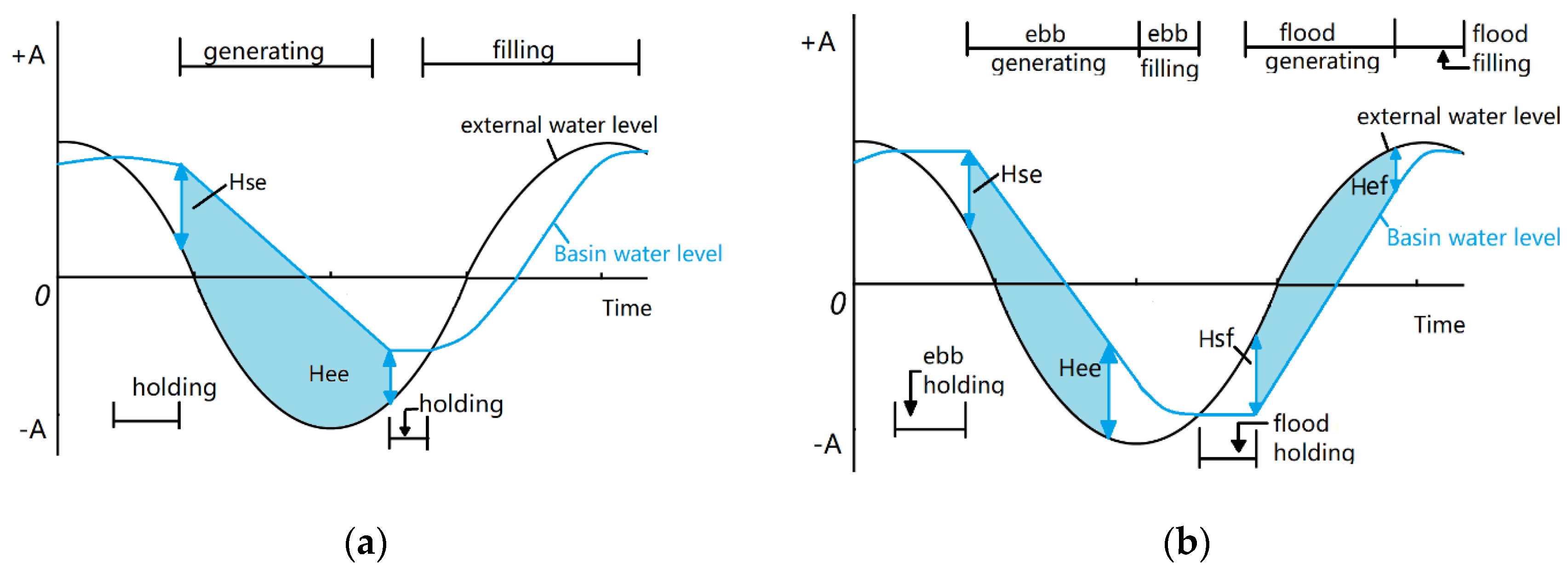
Energies 12 02870 g001
Figure 2. Schematic representation of the operational schemes: (a) One-way ebb generation; (b) a two-way tidal power plant.
Energies 12 02870 g002
Figure 3. Schematic representation of the operational mode (including pumping) of: (a) One-way ebb-generation; (b) a two-way tidal power plant.
Energies 12 02870 g003
Figure 4. Overview of the project elements [24].
Energies 12 02870 g004
Figure 5. Wetted area versus water level.
Energies 12 02870 g005
Figure 6. Energy output: (a) With a constant impounded area; (b) with impounded area varying with water level, in which the Hse/Hee denote the starting/ending generation water elevations.
Energies 12 02870 g006
Figure 7. Andritz Hydro three-blade low head bulb turbine unit [31].
Energies 12 02870 g007
Figure 8. Turbine efficiency calculated from Figure 7.
Energies 12 02870 g008
Figure 9. 3 Schematic illustration of different optimisation methodologies: (a) Full tide optimisation illustrations: every-tide (ET) and every tidal cycle and next (ETN) methods; and (b) half tide optimisation illustrations: every-half (EH) and every half-tidal cycle and next (EHN) methods.
Energies 12 02870 g009
Figure 10. ET model for 10 tides, with the maximum energy point, i.e., most optimised operation, being shown with a red cross.
Energies 12 02870 g010
Figure 11. Operation scheduling of the impoundment, water levels inside the impoundment, and power output comparisons for four neap tides, M_fixed-head, M_ET, M_ETN, M_EH, and M_EHN represent the operation schedule based on fixed head, ET, ETN, EH, and EHN models, respectively, in which 1 to 3 denote sluicing, generating, and holding phase, respectively. Zlw represent the seaside water level. WL_fixed-head, WL_ET, WL_ETN, WL_EH, and WL_EHN represent the basin water level based on fixed head, ET, ETN, EH, and EHN models, respectively. P_fixed-head, P_ET, P_ETN, P_EH, and P_EHN represent the power output based on fixed head, ET, ETN, EH, and EHN models, respectively.
Energies 12 02870 g011
Figure 12. Swansea Bay Lagoon region and bathymetry as included in the depth integrated velocities and solute transport (DIVAST 2-DU) model.
Energies 12 02870 g012
Figure 13. Typical comparison of observed and predicted water levels at L2 (a), L3 (b), and L5 (c).
Energies 12 02870 g013aEnergies 12 02870 g013b
Figure 14. Typical comparison of observed and predicted current speed at L2 (a), L3 (b), and L5 (c).
Energies 12 02870 g014
Figure 15. Typical comparison of observed and predicted current direction from North at L2 (a), L3 (b), and L5 (c).
Energies 12 02870 g015
Figure 16. Water level (a) and current (b) streamlines during the flood generating mode in the 2-D model.
Energies 12 02870 g016
Figure 17. Water level (a) and current (b) streamlines during the ebb generating mode in the 2-D model.
Energies 12 02870 g017
Figure 18. 2-D and 0-D model comparisons between: (a) Water level and power output, in which WL_0-D, WL_2-D and Zlw_0-D, Zlw_2-D denote the basin water level and seaside water level in 0-D and 2-D models, respectively. P_0-D and P_2-D denote the power output in 0-D and 2-D models, respectively; (b) water head difference and energy generated, in which DH_0-D, DH_2-D and Energy_0-D, Energy_2-D denote the water head difference and energy generation in 0-D and 2-D models, respectively; and (c) discharge through the sluice gates and turbines, in which QTB_0-D, QTB_2-D and QSL_0-D, QSL_2-D denote the discharge through turbines and sluice gates in 0-D and 2-D, respectively.
Energies 12 02870 g018
Table 1. Energy generation per cycle for the 0-D model.
Cycle NoStarting Time (h)Ending Time (h)Energy (GWh)Relative Deviation (%)Cycle No.Starting Time (h)Ending Time (h)Energy (GWh)Relative Deviation (%)
160.60421.5019.69−5.57134284.404619.6022.628.46
2421.50781.8020.44−1.96144619.604991.4019.03−8.75
3781.801130.1021.362.42154991.405341.2022.316.99
41130.101489.5019.86−4.77165341.205699.4019.72−5.42
51489.501824.9021.814.60175699.406061.4021.432.76
61824.902197.5019.06−8.59186061.406445.6021.844.75
72197.502534.1022.578.24196445.606804.8019.20−7.92
82534.102892.9019.15−8.14206804.807165.8023.5813.09
92892.903241.8023.3011.76217165.807512.2018.29−12.29
103241.803612.3018.55−11.04227512.207873.2023.8314.29
113612.303924.6022.176.32237873.208221.2019.26−7.63
123924.604284.4017.98−13.77248221.208568.6023.3912.16
Table 2. Optimisation scenarios for second tidal cycle.
ScenarioEnergy (GWh)Change to Fixed-Head Schedule
Fixed-head schedule21.3-
OptimisedET model23.510.5%
ETN model23.610.6%
EH model23.811.9%
EHN model24.012.5%
Table 3. Pumping optimisation scenarios for the second tidal cycle.
ScenarioEnergy (GWh)Change to Fixed-Head Schedule
Fixed-head schedule21.3-
OptimisedETP model26.725.5%
ETNP model26.725.5%
EHP model27.026.7%
EHNP model27.127.2%
Table 4. Analysis of measured and predicted data at L2, L3, and L5.
NoLocationLatitudeLongitudeTermsRMSER2
1L251°31.78′ N003°58.96′ WWater Level (m)0.1110.997
Velocity (m/s)0.0550.832
2L351°33.56′ N003°56.32′ WWater Level (m)0.1360.997
Velocity (m/s)0.0310.774
3L551°31.82′ N003°51.25′ WWater Level (m)0.1470.997
Velocity (m/s)0.0170.787
Table 5. Energy generation comparison between 0-D and 2-D models.
Averaged Duration of Generating in Every Half Tide of the Typical Cycle (h)Average Energy Generated in the Typical Cycle (Gwh)
0-D model1.921.3
2-D model1.919.7
change0%−7.5%
Table 6. Comparison of optimisation scenarios without pumping.
ScenarioEnergy (GWh)Change to Fixed-Head Schedule 2-D (%)Difference between 2-D and 0-D Energy Prediction (%)
2-D Model1 0-D Model
Fixed-head schedule19.721.3-−7.5%
OptimisedET model22.723.515.6%−3.2%
ETN model22.823.615.7%−3.2%
EH model22.823.815.8%−4.3%
EHN model22.924.016.0%−4.6%
1 as shown in Table 2.
Table 7. Comparison of optimisation scenarios with pumping.
ScenarioEnergy (GWh)Change to Fixed-Head Schedule 2-D (%)Difference between 2-D and 0-D Energy Prediction (%)
2-D Model1 0-D Model
Fixed-head schedule19.721.3-−7.5%
OptimisedETP model25.326.728.4%−5.0%
ETNP model25.426.729.0%−4.8%
EHP model25.427.029.0%−5.9%
EHNP model25.527.129.6%−5.8%
1 as shown in Table 3.

