Abstract
As one of the major production facilities in agriculture, a greenhouse has many spatial distributed factors influencing crop growth and energy consumption, such as temperature field, air flow pattern, concentration distribution, etc. By introducing a hybrid computational fluid dynamics–evolutionary algorithm (CFD-EA) method, this paper constructs a micro-climate model of greenhouse with main environmental parameters optimized. Considering environmental factors’ spatial influences together with energy usage simultaneously, the optimal solutions of control variables for crop growth are calculated. A commercial greenhouse located in east China is chosen for the method validation. Field experiments using temperature/velocity sensor matrix are carried out for CFD accuracy investigation. On this basis, the proposed optimization method is employed to search for the optimal control variables and parameters corresponding to the environmental Pareto frontier. By the proposed multi-objective scheme, we believe the method can provide set point basis for the design and regulation of large/medium-sized greenhouse production with high spatial resolution.
1. Introduction
Greenhouse production plays an important role in the development of modern agriculture, especially in densely-populated areas with tight land, such as eastern China. The environmental conditions in greenhouses are essential for crop growth, pest/disease prevention, energy saving, etc. For most active or passive greenhouses, appropriate environmental parameters for crop growth are assessed based on the analysis of environmental factors as lumped parameters [1]. Meanwhile, for large/medium-sized greenhouses, the environmental parameters at the crop growing area are not equal to the values at the sensors’ location. For more accuracy, parameters such as temperature, ventilation rate and concentration, should be considered based on a precise micro-climate model considering the spatial distribution inference.
Improvements in computing facilities together with theoretical and experimental studies increased our understanding of the biophysical process in a greenhouse system. At present, computational fluid dynamics (CFD) has been widely applied for greenhouse climate simulation [2,3,4,5,6]. Ould Khaous et al. [3] applied CFD to greenhouse ventilation efficiency evaluation. Results showed that air velocity at plant level varied from 0.1 to 0.5 according to opening configurations and compartment positions, whereas air temperature differences varied from 2 to 6 C. Similarly, Lee and Short [2] used CFD to evaluate natural ventilation rates and airflow distributions in a multi-span greenhouse; Santolini et al. [5] studied the effect of shading screens on airflow patterns within the greenhouse through CFD simulations. To relieve computational burden of CFD simulation, alternative models based on an artificial neural network (ANN) [7] or support vector machine (SVM) [8] are also reported for greenhouse system analysis. For these data-driven models, the modeling error issue could not be ignored.
High resolution modeling may facilitate precise regulation. To search optimal parameters of greenhouse environment, researchers employed manual CFD simulations for evaluation of candidate parameters. Tong et al. [9] used CFD method for span dimension selection of Chinese solar greenhouses. Three groups of span configurations (10 m, 12 m and 14 m) were investigated using CFD simulations and their characteristics including solar heat gains, heat losses and temperature distributions were analyzed. Wang et al. [10] used CFD method for thermal performance improvement of solar greenhouses. Three solar greenhouses with different north walls were simulated and analyzed; to achieve the best north wall thickness of the greenhouse, Zhang et al. [11] carried out 18 case studies based on CFD simulation. An evaluation model using weighted entropy and fuzzy optimization scheme was then employed for decision making; to optimize the vent dimension and position in greenhouse design, He et al. [12] investigated all effects of different back wall vent configurations by two groups of CFD models.
By contrast with solution searching through manual simulations, an interactive optimization scheme using a hybrid simulation–optimization method has superior performances in terms of computation efficiency, solution accuracy, and design convenience. In the field of building enclosure optimal design, commercial middleware such as GenOpt [13] and OpenFOAM [14] have been used in various scenarios. Asadi et al. [15] combined building energy simulation program with GenOpt to regulate energy usage and thermal comfort of a residential building. Futrell et al. [16] used similar hybrid method to search optimal solutions of daylighting and thermal performance of a campus building. Liu and Chen [17] combined CFD simulation with genetic algorithm (GA) through OpenFOAM for optimization of indoor environmental parameters.
Compared with residential buildings, the optimization task of greenhouse environment is still challenging. Firstly, there are multiple optimization goals within greenhouse systems, such as crop quality, economic benefits, energy usage, etc.; secondly, many environmental variables contribute to the goals of optimization, for instance, air temperature, illumination intensity, wind speed, soil fertility, etc.; most differently, the optimization goals of the greenhouse environment are not constant, but changing with space and time. In this study, we design an interactive optimization scheme for environmental performance regulation in greenhouse system. To facilitate the combination of existing CFD simulation and proper optimization algorithms, an efficient interactive module is realized, which links CFD and Matlab software through data exchange mechanism. On this basis, the paper aims to understand how the spatial distribution of environmental factors influence crop growth as well as to present a multi-objective optimization case study based on the hybrid computational fluid dynamics—evolutionary algorithm (CFD-EA) method. A summer’s 720 Venlo type commercial greenhouse located in east China is chosen as the case scenario. The temperature fields and airflow patterns at essential sections are validated by field experiments. Three indexes, i.e., proper temperature distribution, proper concentration, and electrical energy consumption are chosen as optimization objectives. Simulation study provides precise set points at one selected period for feedback regulation within the greenhouse system. Results will show the feasibility and high resolution of the hybrid optimization method.
The rest of the paper is organized as the following. Section 2 provides the details of the proposed optimization method. Section 3 depicts the construction of the CFD model for the real greenhouse. Accuracy validation with field experiment is presented in Section 4. Section 5 provides the optimization procedure and results. Some concluding remarks and future works are given in Section 6.
2. Method
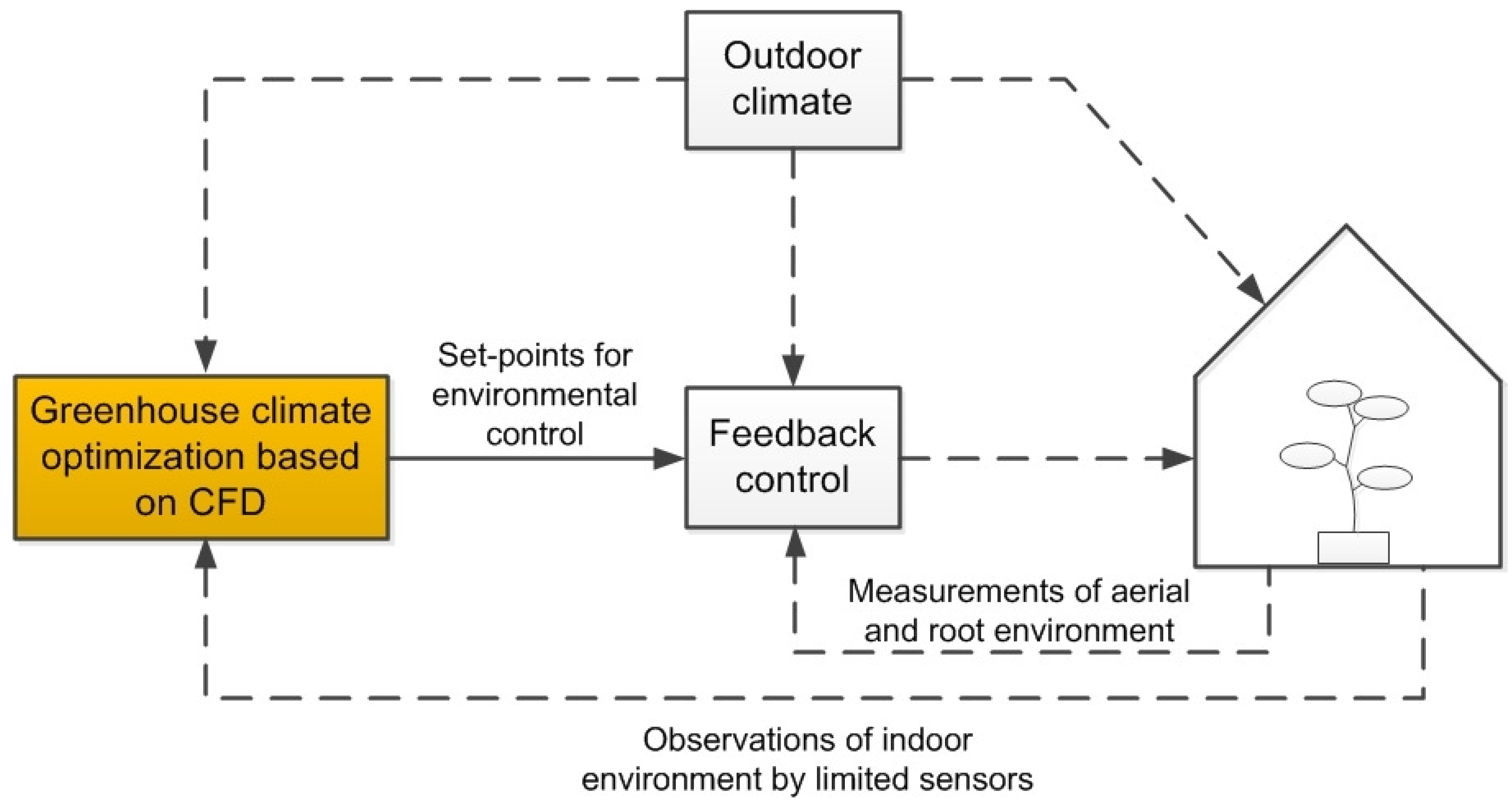
Generally, the greenhouse climate management can be resolved into two dynamic processes: slow crop growth dynamics and relatively fast greenhouse climate dynamics [1,18]. For fast climate dynamics, the set-points of the greenhouse environmental variables such as air temperature, humidity and concentration, should be decided in advance by the grower or computer systems. Once these set-points are decided, the desired climate in the greenhouse can be achieved by proportional–integral (PI) or other classic feed-back control methods. However, these set-points are usually time-varying and spatially distributed. In recent years, many optimal control schemes have been reported for such greenhouse climate control problems [18,19,20]. The environmental parameters’ spatial feature is seldom mentioned, which is important for crop growth and energy saving in large and medium-sized greenhouse. Figure 1 describes the basic block diagram of the climate control procedure and the highlighted optimization part is the focus of this study.

Figure 1.
A block diagram of the climate control procedure.
2.1. Interactive Optimization Scheme
Considering the spatial influences of environmental parameters, CFD simulation is the most accurate way of modeling. Taking advantage of the current high-speed development of computing technology, hybrid simulation–optimization has been widely used in the field of building enclosure optimal design and operation. Combined with previous reported interactive optimization methods [17,21,22], we propose a set of greenhouse environment optimization solutions.
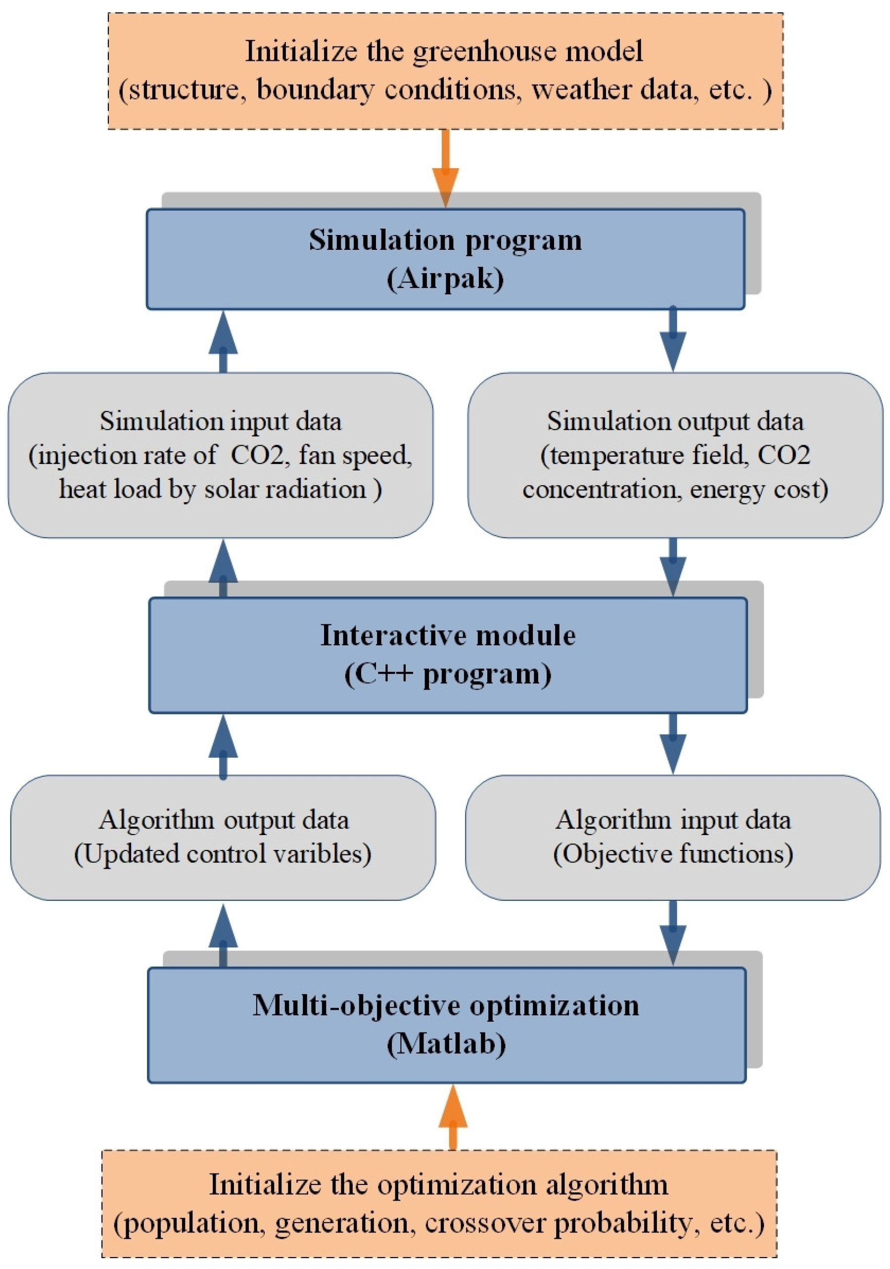
Using a validated CFD model, a global optimization scheme was combined for greenhouse environmental parameters optimization. At each iteration of optimization, distributed indoor micro-climate model was calculated by CFD (Airpak3.0.16 with Fluent engine), and the results including temperature field, concentration, and energy consumption were format converted and transmitted to the optimization scheme through a middle module; in order to adapt to the features of the greenhouse environment optimization, we developed a middleware (C++ program) instead of directly using commercial softwares [21].
The spatial distributions of multiple environmental parameters are non-linearity, discontinuity and with high uncertainty. EAs working with a population of stochastic solutions can be used to find multiple Pareto-optimal solutions in one single simulation run. For this study, the non-dominant genetic algorithm with elite strategy (NSGA-II) [23] was chosen, which can find much better spread of solutions and better convergence near the true Pareto-optimal front compared to its previous version. This algorithm is realized in the Matlab environment. After finding out the Pareto frontier of main environmental parameters, the corresponding control variables were updated and exchanged back to CFD for next simulation. The interactive optimization loop continues until the stop criteria is reached.
Figure 2 describes the basic flow chart of the proposed interactive scheme.
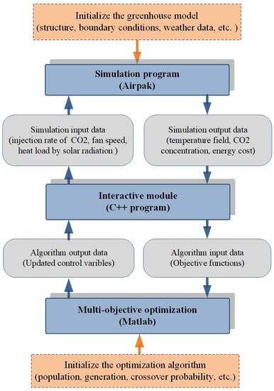
Figure 2.
Interactive optimization scheme.
In the scheme, the C++ program is applied for data exchange between CFD and optimization algorithms. For each iteration of optimization algorithm, the data exchange module works as the follows.
| Start |
| Read control variables from Matlab; |
| Delete old model file of Airpak (); |
| Create new model file () according to template file’s format |
| () and update the control variables; |
| Call Airpak to run the CFD simulation; |
| WHEN the CFD simulation meets the stop criteria |
| Save the results and transfers them from Airpak to Matlab by files; |
| End |
2.2. Multiple Objectives and Control Variables
For greenhouse production, the optimal indoor environmental parameters have characteristics of time-varying and spatial heterogeneity, especially for the uneven planting of crops. The indoor environmental parameters that this article focuses on include air temperature, concentration and corresponding energy consumption.
2.2.1. Objectives
The suitability of environmental temperature is a primary assessment criterion for crop growth. In a greenhouse, solar radiation and other external factors affect indoor temperature dramatically. How to reduce external disturbance and improve the indoor temperature distribution is an important issue in large greenhouse systems. For greenhouse production, the ideal temperature field is a function of time and crop growth. In this paper, we refer to the crop growth model based on temperature management technology [24,25], and choose one period in summer for the later case study.
Another important factor affecting crop growth is indoor concentration. The optimum concentration in the greenhouse depends on several factors: crop photosynthetic rate, loss rate, indoor temperature, and cost. A benchmark curve of concentration in one day was referred [24], and one segment was chosen for the later case study. Although relative humidity also has a great influence on crop growth, it was not controlled in this study because its value is usually greater than 80% in summer of east China, and the spatial difference can be ignored.
Three assessment indexes for the multi-objectives optimization were set, which were temperature distribution index, distribution index, and energy consumption index. It should be noted that the essential economic cost for greenhouse crop production is heating energy. Considering the climate characteristics of eastern China in summer (air temperature is up to 40 C), we only chose the economic costs of electricity and injection representing the main energy consumption in this study. The three indexes are formulated below,
where and represent values at / sampling points in interested crop areas. and are idea values of temperature and concentration in crop areas. is the total number of sampling points in crop areas and is the number of fans. and are the overall volumetric flow rate of supply air and () respectively. is the pressure rise through the supply fan (Pa) and is the fan efficiency. and are prices of electricity and at local market. The parameters and are mass fraction and density of injected . is the duration time of the regulation.
2.2.2. Control Variables
To achieve these three objectives, three control variables (setting points) were set in the optimization scheme including fans’ speeds, injection rate of , and heat load of solar radiation. According to previous research [18,19], these variables have obvious effects on indoor micro-climate. Since the optimization is simulation based, the heat load of solar radiation is assumed to be changed by the shading coefficient, and the practical implementation of these control variables are beyond the scope of the article.
2.3. Online–Offline Strategy
To derive the multiple environmental parameters’ steady fields of the greenhouse, the full CFD procedure may be very time consuming. This further makes the computational cost of interactive optimization very expensive.
For efficient computation, an online–offline scheme was employed. In the offline phase, the full CFD simulations were executed to calculate the original greenhouse model with precise solutions. In the online phase, on the basis of ensuring convergence, the mesh was simplified and the converge conditions are relaxed to acceptable extents. The purpose of this setting was to relieve the calculation burden and improve the optimization efficiency.
3. Model Construction Using CFD
Since the summer weather in east China is very hot, crop growth and energy usage are significantly affected by spacial distributed micro-climate factors of the greenhouse such as temperature field and air flow distribution. In this study, we choose a medium-large greenhouse in east China for model construction and method validation.
3.1. Structure of the Venlo Greenhouse
The greenhouse for investigation is located in Zhenjiang, Jiangsu Province (32.080248(N), 119.503427(E), 50 m(ASL)). The greenhouse has three spans with the length × width: 40 m × 18 m in total (720 ). The roof goes along the north-south direction. The eaves height is 3.175 m and the roof height is 5.0 m. The main surrounding shelter and roofing materials are polycarbonate (PC) sunshine plates (thickness 4 mm, light transmission rate 87%). Three ventilation fans are installed on the north wall of the greenhouse (one fan each span). To facilitate experiment validation of temperature and airflow distributions, the greenhouse is almost empty and no crops are growing inside (We carried out the experiment after weeding, but the weeds grown out fast within two weeks during the experiment. In the CFD simulation, the latent transfer and water vapour exchanges of weeds are not considered). The location and profile of the greenhouse are shown in Figure 3.

Figure 3.
The location and structure of the target greenhouse.
3.2. CFD Model Construction
In the greenhouse thermal procedure, temperature distribution is thermally coupled with airflow field, which is mainly governed by the incompressible Navier–Stokes equations. Boussinesq approximation is applied for representing buoyancy effect in the CFD simulation. The nondimensional form of basic conservation equations are shown below:
in the domain , where represents a spatial domain, is a unit vector in the direction of gravitational acceleration, the Prandtl number , Grash of number , and Reynolds number .
Considering the turbulent characteristics of the airflow during the ventilation procedure, renormalization group model (RNG) was used to predict indoor microclimate of greenhouse, which was reported more accurate than standard model with weak air velocities [26]. The discrete ordinates (DO) radiation model was chosen for indoor radiation simulation, and the effect of solar radiation on the room temperature is simplified using Airpak’s solar load model. The latent transfer and water vapour exchanges of weeds are ignored.
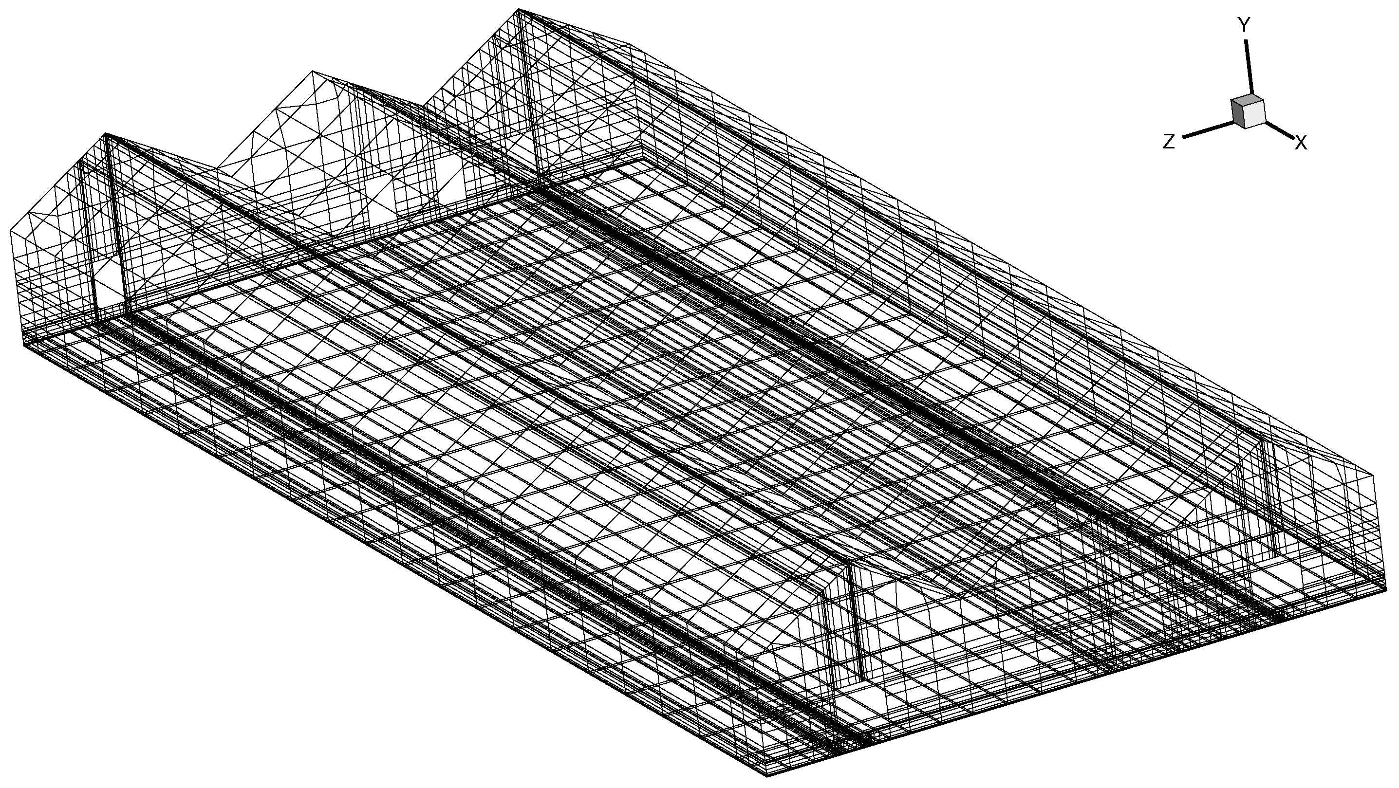
Airpak 6.3 is the simulation tool based on a finite volume method as a Fluent engine. The calculation domain consists of two parts: indoor area (40 m × 18 m × 5 m) and outdoor area (200 m × 100 m × 25 m). In early summer in eastern China, the main heat source of greenhouse comes from outdoor heat radiation. The ventilation condition was set as negative pressure ventilation (the velocity inlet type is applied for fans, and the zero gradient boundary condition (outlet type) was applied for windows). The roof is considered as semitransparent medium, and the surrounding shelter’s absorption coefficient of radiation is set as a constant. The basic parameters setting and initial conditions are listed in Table 1. There were a total 348,134 unstructured hexahedral mesh elements generated for model calculation. The structure of the greenhouse model with mesh is shown in Figure 4.

Table 1.
The basic parameters setting for computational fluid dynamics (CFD) simulation.
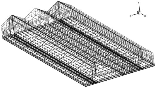
Figure 4.
The structure of the greenhouse model with mesh.
3.3. Simulation Results
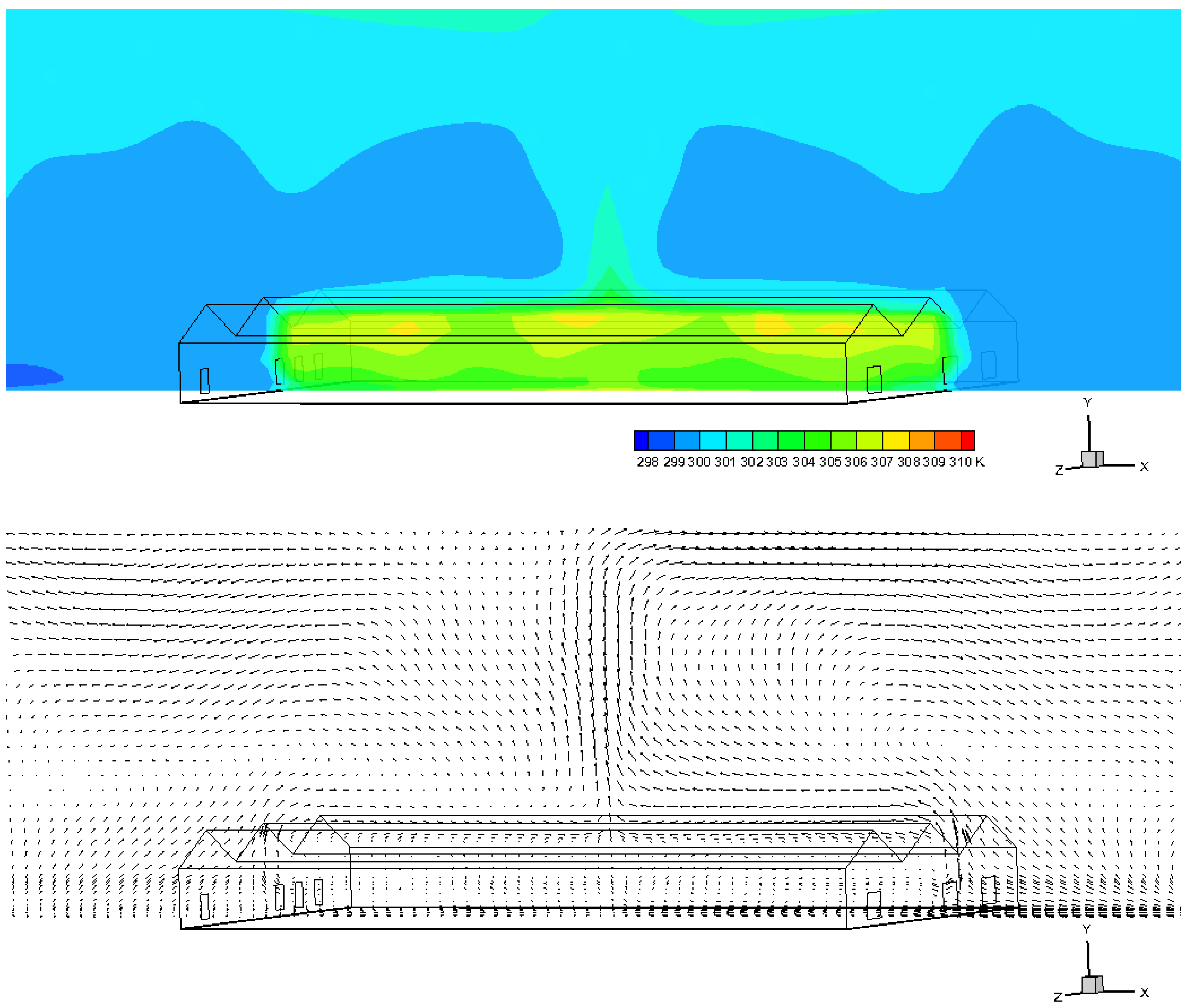
Figure 5 provides steady temperature contour and airflow vector field at one vertical section facing the window and fan. From the figure, it is seen that indoor temperature and airflow are not evenly distributed. The assumption of “well mixed” does not exactly fit into the real situation, which was also reported by many previous literature [2,3,5]. Concretely, at noon during a warm day (May in east China), the temperature in the upper part of the greenhouse was generally higher than the temperature in the lower area because of the outdoor heat radiation through the sunshine-plate roof. The temperature near the natural ventilation windows was lower than the temperature of middle area because the average temperature inside the greenhouse was higher than outside at noon. Because of the negative pressure ventilation by three fans, the lower air flows faster than the upper part.
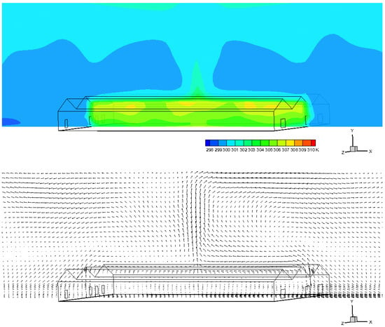
Figure 5.
Temperature (top) and airflow (bottom) fields at the vertical section (Z = 15.5 m).
4. Model Validation with Field Experiment
4.1. Experiment Setting
To validate the CFD model’s accuracy, field experiments are employed for this study. Both temperature and air speed measurements are executed in this case study.
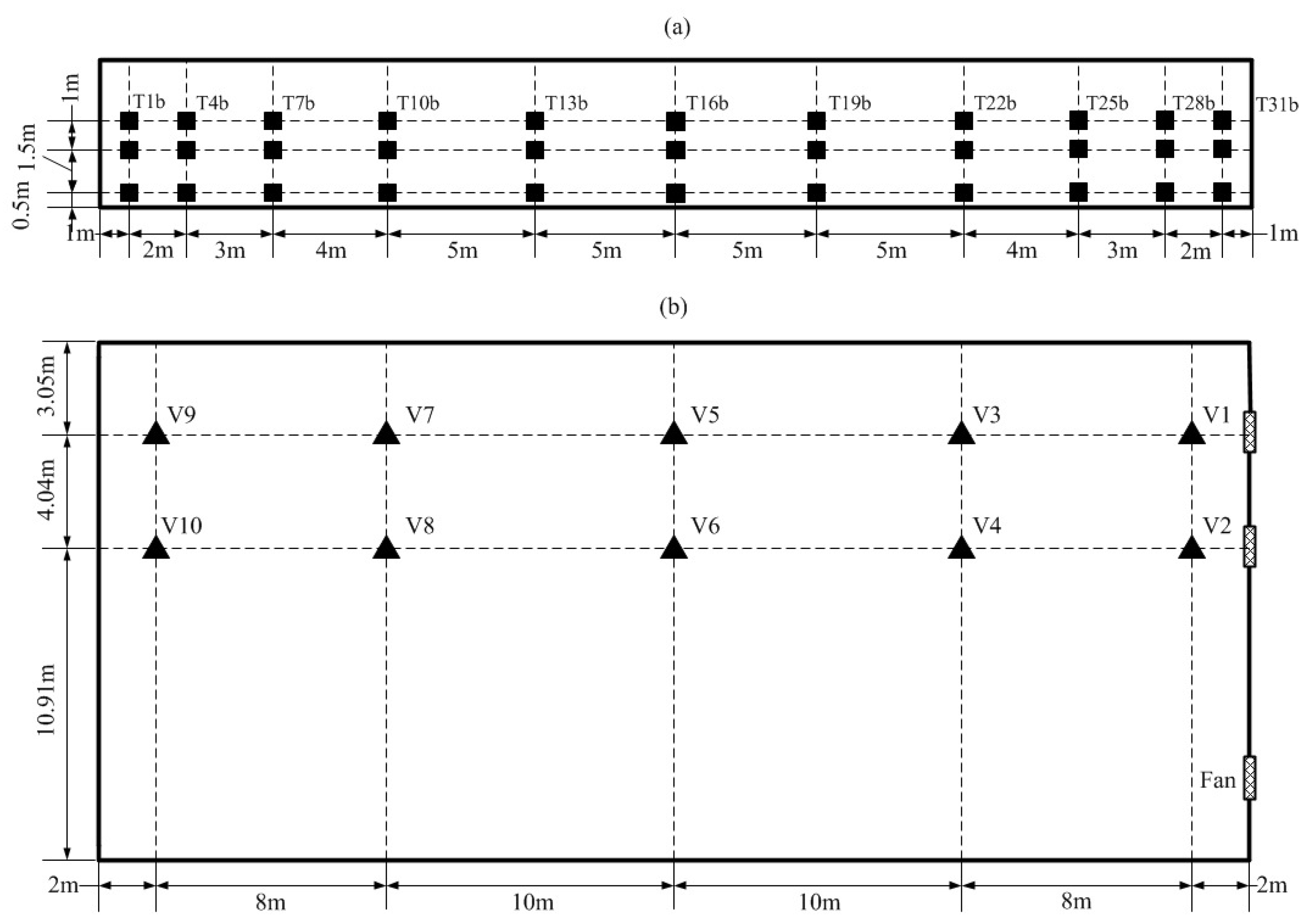
There were 33 temperature sensors () forming a measurement matrix in single vertical section from south to north (length direction × height direction: ). The section location was selected facing the middle fan (Z = 7.089 m). At each height, there were 11 temperature sensors uneven distributed: sparse in middle area, dense near boundaries. The side view of the 2D sensor matrix from east direction is provided in Figure 6a. Airflow patterns were also investigated by 20 observing points () at two vertical sections with two heights (: 0.7 m, : 1.6 m). The top view of the air velocity sensor matrix is provided in Figure 6b.
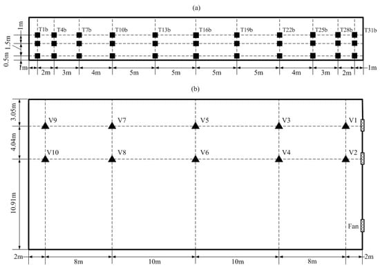
Figure 6.
Locations of temperature and air speed sensors: (a) the side view of temperature sensor matrix, (b) the top view of the air velocity sensor matrix.
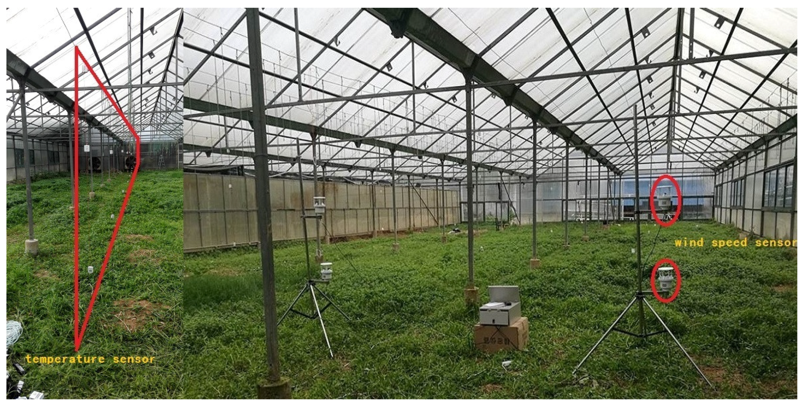
The type of temperature sensor is TP4029POS, C; the type of ultrasonic three-dimensional wind speed sensor is WS-A2, m/s. The solar radiation intensity and outside temperament/airflow speed are also recorded by meteorological station. The experimental scene is shown in Figure 7.
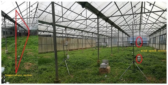
Figure 7.
The experimental scene in the Venlo type commercial greenhouse.
4.2. Experiment Results
The experiment was carried out at 12 a.m.–15 p.m., 5 May 2017. At this time period, the outside temperature was relative high, which is helpful to observe obvious temperature gradient distribution. Each sensor sampled ten times at the same location (1 min interval), and the average results were recorded and saved by wireless data collector. Under natural and mechanical ventilation conditions, temperature measurements are employed using above experiment settings. Detailed data is provided in Appendix section in Table A1 and Table A2. Under mechanical ventilation condition, the air velocity field is also sampled by wind speed sensors. Results are shown in Table A3.
Figure 8 shows the 2D temperature distributions under natural and mechanical ventilation conditions. In the figure, the obvious temperature gradient distribution in vertical section is observed like simulation results. Moreover, compared with natural ventilation results (Figure 8a), mechanical ventilation (Figure 8b) made the indoor temperature more even, especially at the lower area. This homogeneous distribution of temperature was better for crops production in greenhouses. Using absolute error percentage formula (), Figure 8c shows the percentage of the 2D temperature difference between experiment and simulation results in mechanical ventilation condition.
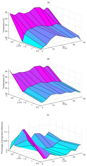
Figure 8.
Results of 2D temperature measurements: (a) natural ventilation, (b) mechanical ventilation, (c) percentage of temperature difference between experiment and simulation.
For model validation, simulation results are compared with experiment results in both natural and mechanical ventilation conditions. The average errors of temperature simulations in different conditions are less than 15%. Due to the sensor accuracy limitations, the air velocity field is hard to validated accurately. The average errors are about 20%. It should be noted that the errors are also partly due to the ignoring of the latent transfer and water vapour exchanges of weeds cover.
5. Multi-Objectives Optimization of the Greenhouse Environment
5.1. Optimization Setting
On the basis of the experiment validation, the optimization case study using the proposed interactive scheme was employed in this section. The optimization focuses on solving two problems: (1) how to find out multiple variables’ optimum setting points according to multiple environmental requirements? (2) For local planting areas, how to adjust environmental variables with high spatial resolution to find the balance of energy saving and environment suitability?
During summer in east China, the indoor temperature at noon is higher than 45 , which is harmful to crop growth. To find out the optimal heat flux of the roofs and the ventilation speeds of fans in the greenhouse, we choose an optimization scenario of summer noon (25 July, 10:00–14:00), and an ideal temperature is set (306 K) according to Section 2.2’s discussion.
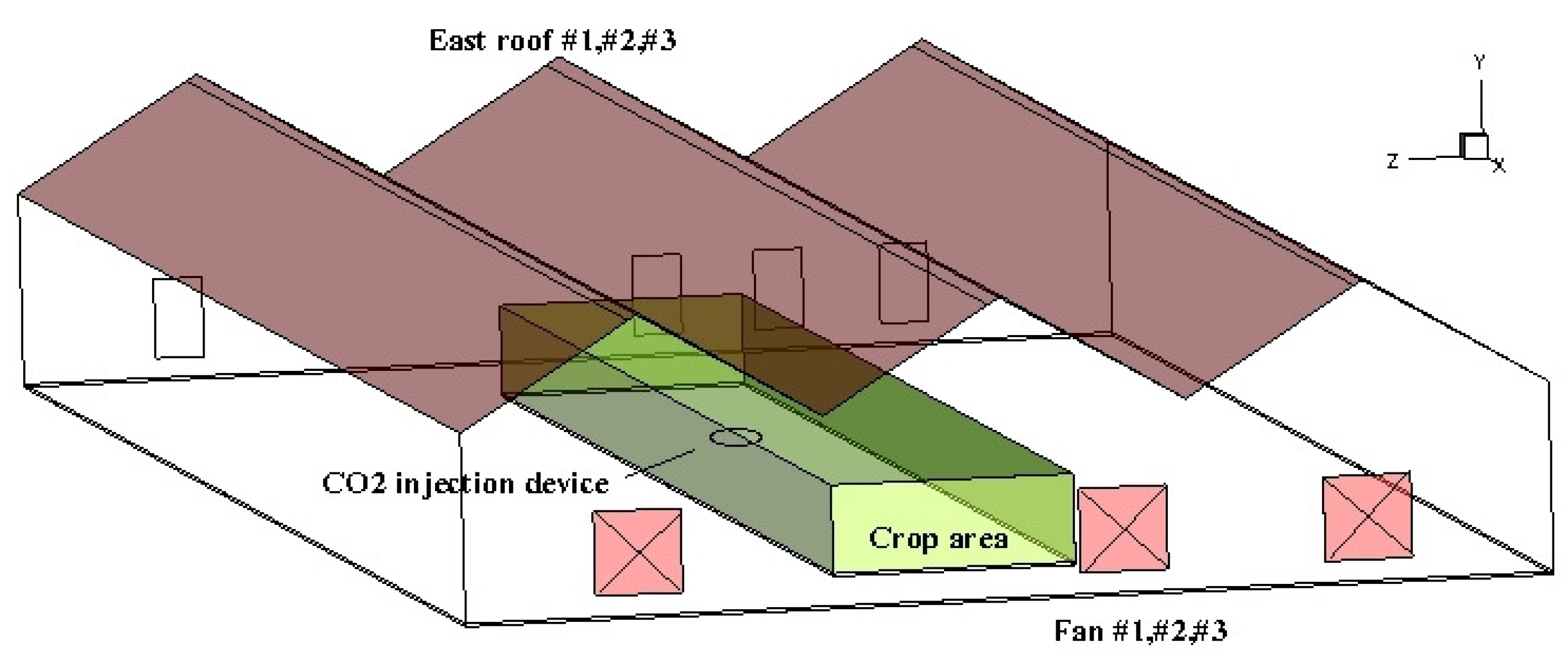
The control variables include: (1) the speeds of three ventilation fans on the north wall (m/s), (2) the injection rate of the simulated device at the center of the greenhouse (m/s), and (3) the simulated heat loads of solar radiation on the east roofs (). The simulated crop growing area ( 30 m × 4 m × 1.5 m) and the three kinds of control devices are shown in Figure 9.
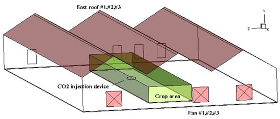
Figure 9.
Profile of the control variables and simulated crop area in the greenhouse.
In addition to Equation (2), The CFD solver uses the multi-species transport model to simulate concentration variation, and the detailed equations and panel setting can be found in Airpak manual [27]. For simplicity purposes, we only recorded the value of spacial concentration in simulated crop area, but the photosynthetic/respiration of crops are not considered in this case. The multiple objective indexes including temperature, concentration, and energy consumption are already described in Section 2, and the related parameters in the formulas are listed in Table 2. In this table, the variation ranges of the control variables are also specified.

Table 2.
Main parameters of the optimization case.
We realized the multi-objective based genetic algorithm (NSGA-II) on the basis of Kalyanmoy Deb’s report [23]. According to the literature analysis and to meet a trade-off with available computational capacity, the population size and maximum number of generations are chosen as 25 and 10, respectively. The online–offline strategy described in Section 2 was applied for computational efficiency improvement. Table 2 specifies the main parameters of NSGA-II for this study.
The computer used to run the simulation is an Intel Core E3 (4 cores, 3.2 GHz) with 16 GB of RAM and the whole optimization procedure requires about 84 h to obtain the Pareto frontier.
5.2. Results and Analysis
5.2.1. Objective Space Analysis
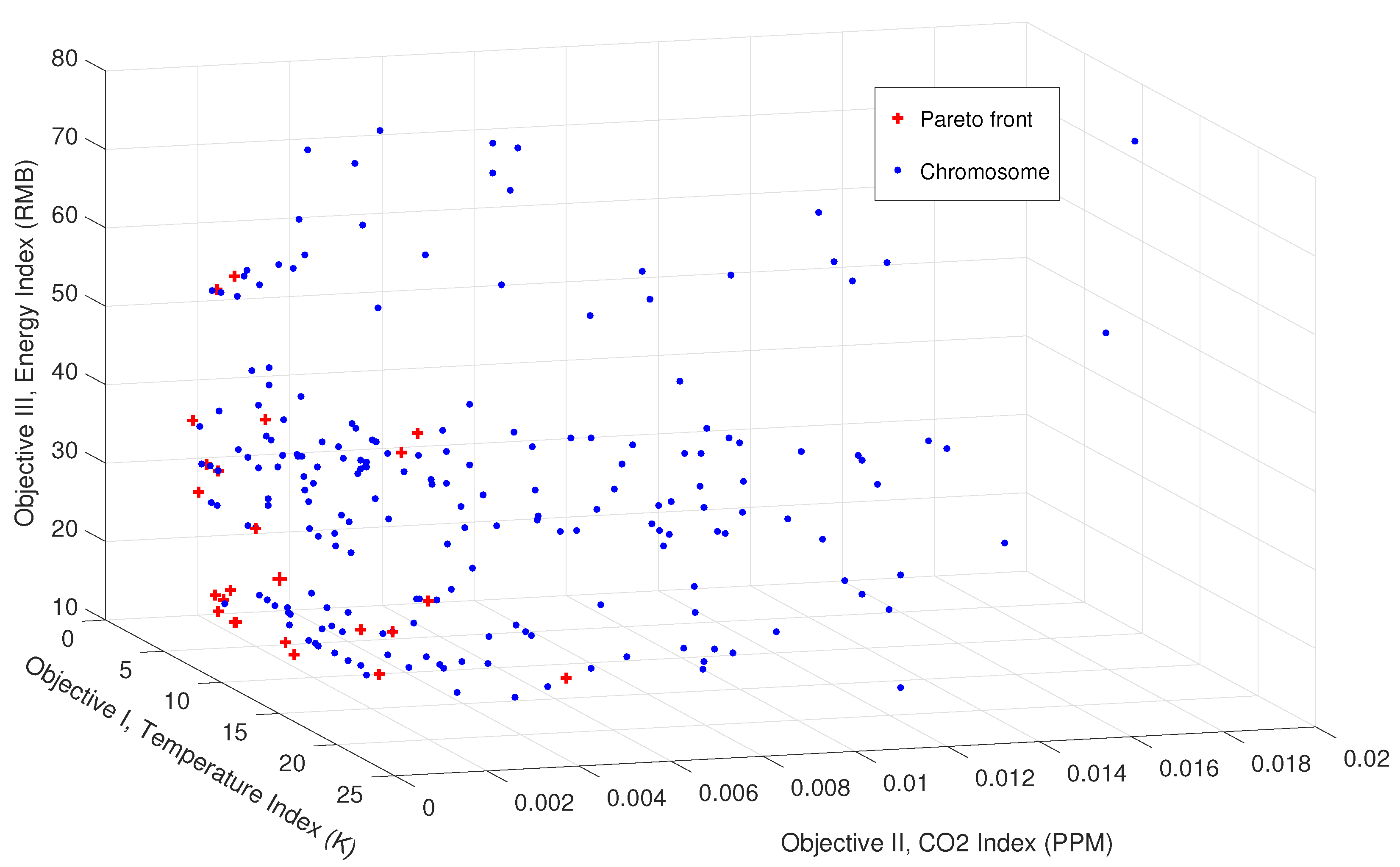
The results of the multi-objective optimization are shown in Figure 10. From a total of 243 chromosomes, 25 pairs of chromosomes of the last generation identified by the NSGA-II algorithm belong to the Pareto frontier. It is noted that seven chromosomes of total 250 are abandoned because of the CFD convergence issue. From the figure, we can find that the target sets represented by particles spread toward the optimal directions. Each particle performs differently with respect to the individual objective indexes. Concretely, among the best 25 solutions, the variation of the index of was [5.08, 20.90] (K), the variation of the index of was [0.0, 0.0055] (ppm), and the variation of the index of was [17.4, 59.9] (CNY).
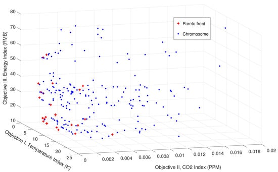
Figure 10.
Tri-dimensional projection of the multiple objectives represented by particles.
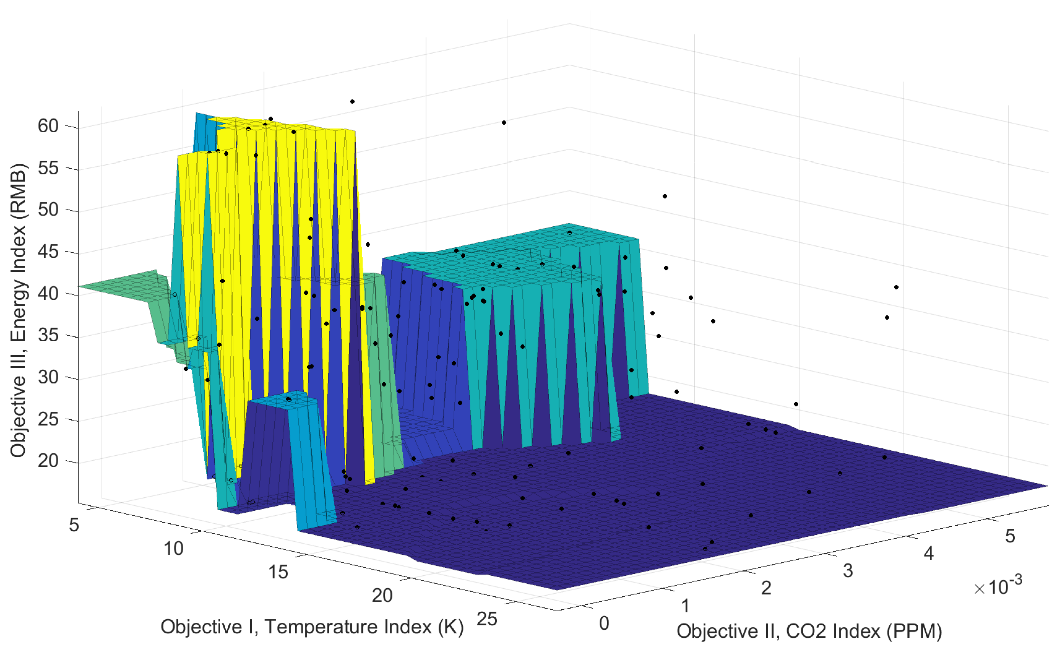
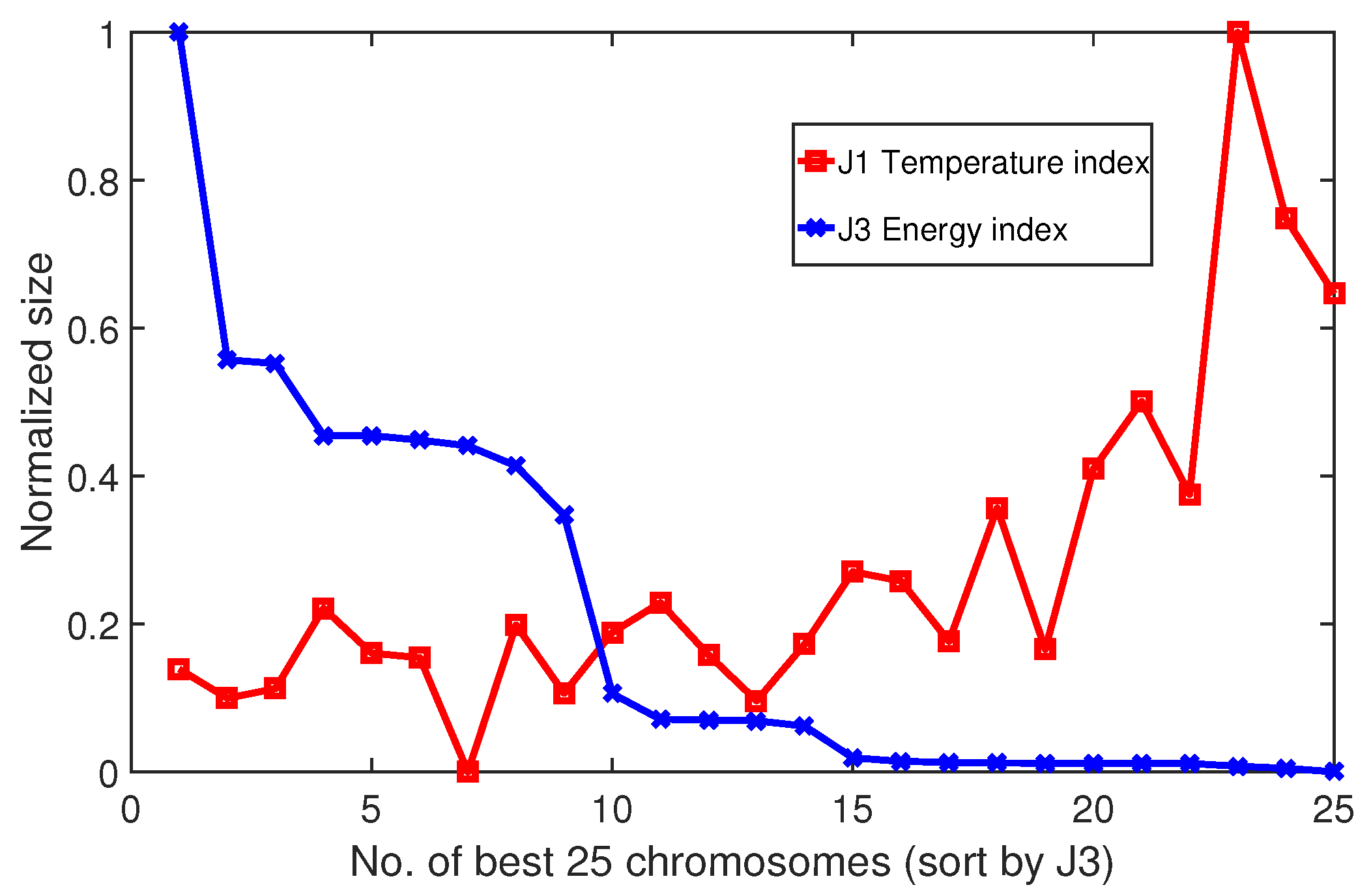
By narrowing down the scope appropriately, we also fit an optimal surface using nearest neighbor method [28], which is shown in Figure 11. In this figure, we can roughly observe the distribution characteristics of the optimal solutions more directly. Basically, as the requirements of environmental indexes (distributions of temperature and in this study) became more stringent, the energy consumption rose sharply, which was consistent with the results of previous studies. If we separately extract temperature and energy cost indexes and plot, they show a significant negative correlation that is shown in Figure 12.
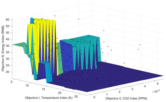
Figure 11.
Fitting surface of optimal solutions using nearest neighbor method.
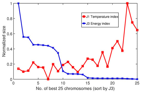
Figure 12.
Negative correlation between temperature and energy cost indexes (25 pairs of chromosomes belonging to the Pareto front).
5.2.2. Control Variable Space Analysis
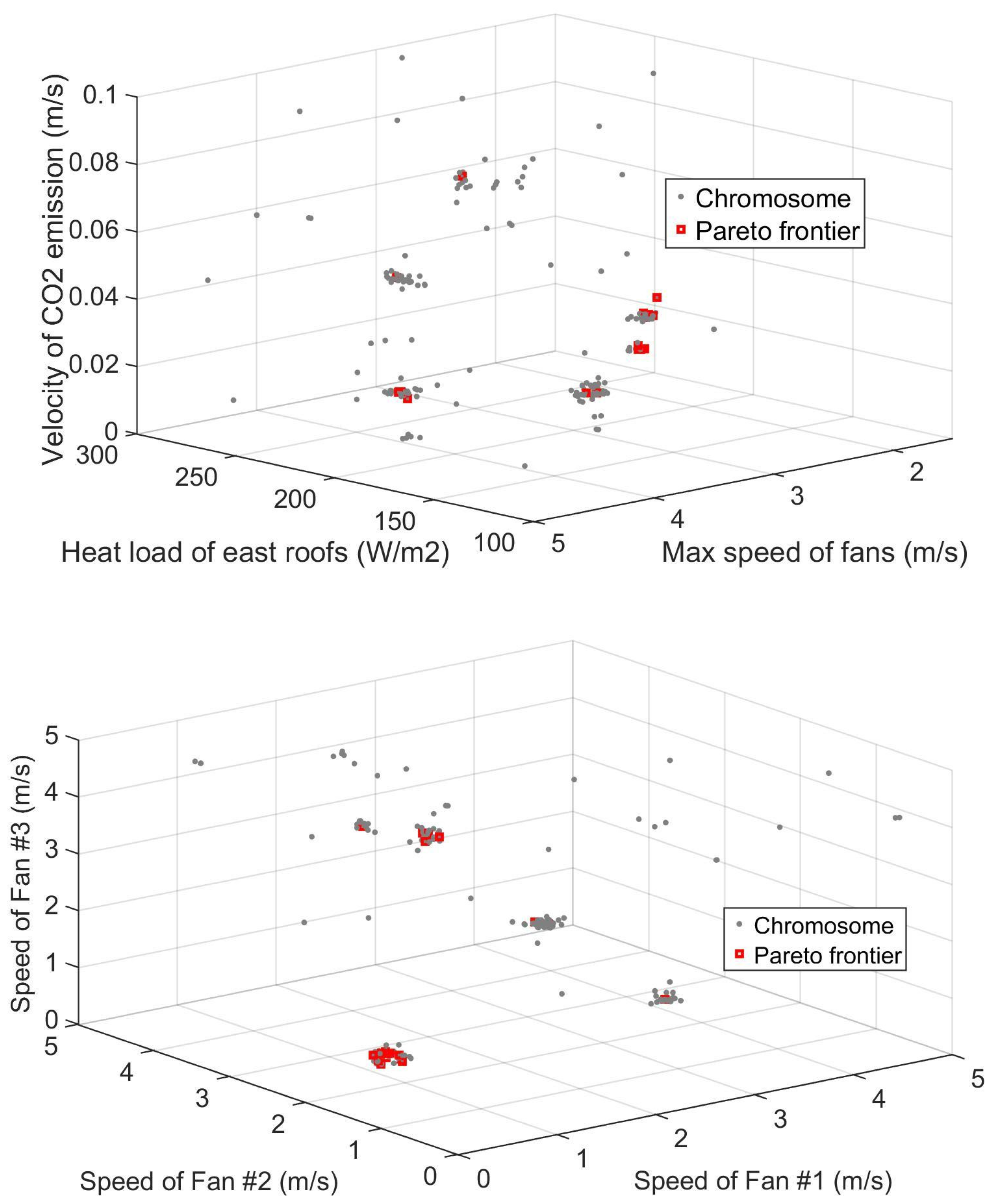
The multiple objective optimization scheme also provide the optimal control variables that are recorded in Figure 13. In total, five different control quantities were divided into two tri-dimensional projections. In the top projection, three main control variables, i.e., heat load of roofs, speed of three fans, and velocity of emission are selected. The variables were clustered in several groups representing different searching orientations of the objective functions. Quantitatively, corresponding to the best 25 solutions, the variation of roofs’ heat load was [154.56, 291.86] (), the variation of fans’ speed is [1.61, 4.63] (m/s), and the variation of emission’s velocity was [0.010, 0.077] (m/s). Note that the maximum speed values of three fans (Fan ) are extracted for this subgraph, and each heat load of the east roofs (Roof ) remains the same in this case study.
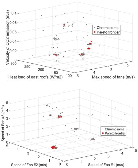
Figure 13.
Tri-dimensional projections of the multiple control variables represented by particles (top projection: emission speed - heat load of roofs - max speed of fans; bottom projection: speed of fan ).
In the bottom subgraph of Figure 13, the individual speeds of three fans are chosen and shown in the form of tri-dimensional projection. From the subgraph, it is found that three fans’ speeds are different because of the relative positions to the crop area. Due to the constraints of energy cost index, the fans’ speeds do not tend to be maximum even at noon in summer. For heat-resistant crops, this was an optimized choice. But for heat-sensitive crops, the weights of energy cost and temperature indexes must be further improved, otherwise the results cannot be adopted in real situation.
5.2.3. Full Simulation of Optimized Greenhouse Model
After the optimization, a steady CFD simulation is carried out using one of the best 25 solutions from the 3D Pareto frontier. Considering the temperature, , and the energy cost in a balanced way, we choose the following pair of control variables: The heat load of east roofs is 154.56 ; the speeds of three fans are 3.56 m/s (Fan ), 3.448 m/s (Fan ), and 1.228 m/s (Fan ); the velocity of emission is 0.021 m/s.
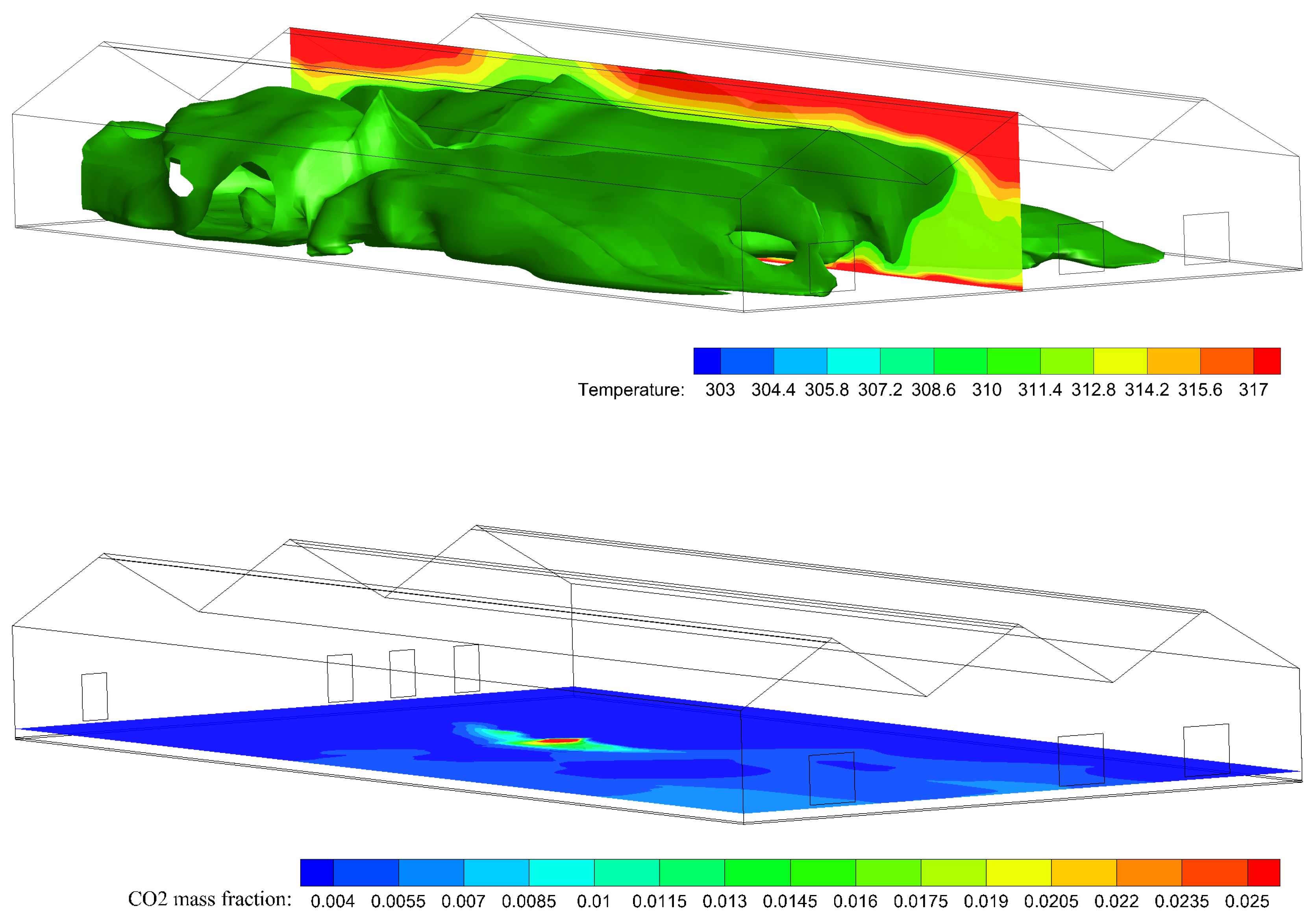
To roughly describe the resulted temperature distribution of this solution, we record the main temperature contour at center plane in Figure 14 (top). Although the ideal value in the temperature index was set at 306 K, a iso-surface of 311 K (38 ) is drawn in this figure considering the heat resistance of crops. From the iso-surface, we can find that most of controlled area’s temperature is below 38 , and the temperature near the roof (above three meters height) rise sharply because of the solar radiant heat. In the bottom sub-figure, we also record the resulted distribution at 0.3 m height. Quantitatively, the average error from standard value (1000 ppm) within crop area is less than 0.005 ppm.

Figure 14.
Resulted temperature contour at center Z plane combined with iso-surface of 311 K (top), and fraction distribution at 0.3 m height (Y plane, bottom).
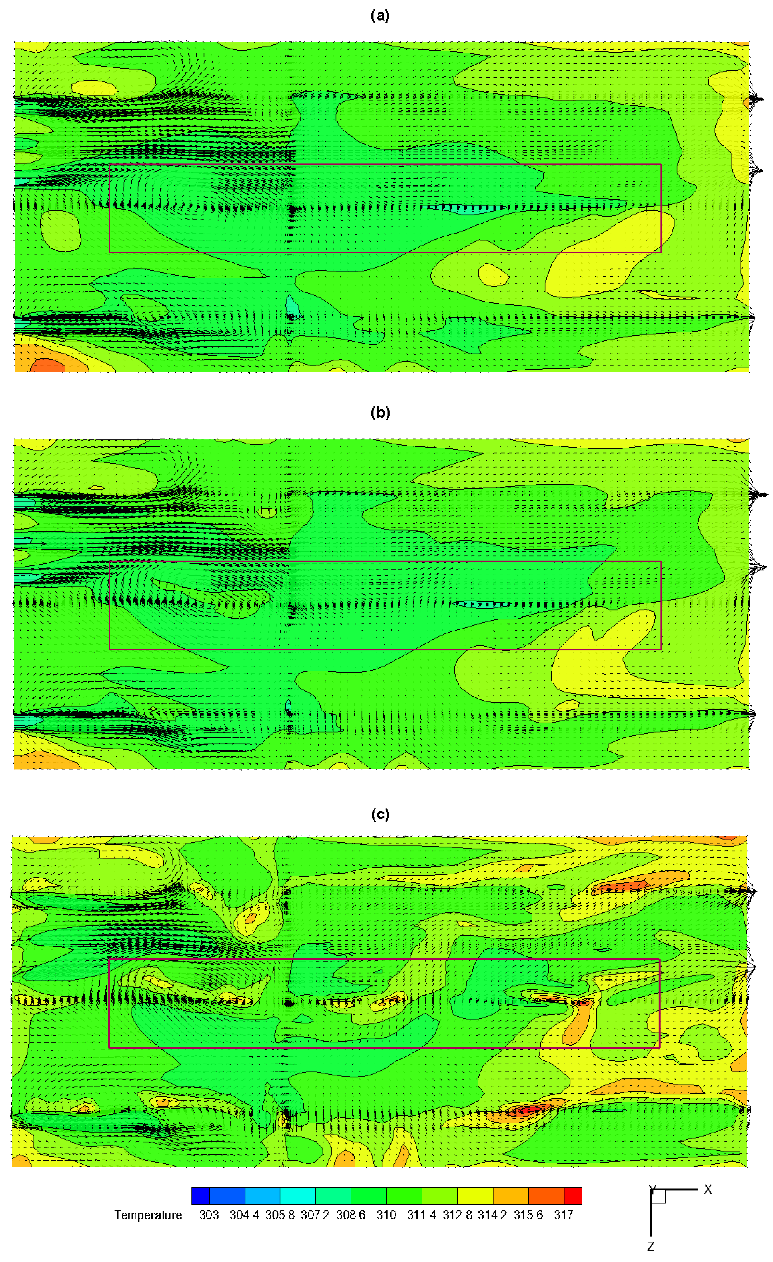
To describe the temperature distribution’s feature of crop area, we also extract three temperature fields at different heights (1.5 m, 1.0 m, 0.3 m) and record them in Figure 15. From the figure, it was found that the temperature values within the most crop area (red rectangle) are between 35 and 37 . This was a result of compromise between environmental parameters and energy usage by multi-objective optimization. Note that the results were based on the premise that keep the ventilation design of the greenhouse unchanged, and some boundary conditions were simplified for simulation iterations.
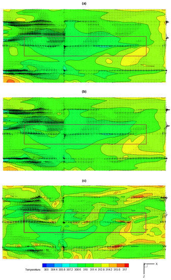
Figure 15.
Temperature contours and air velocity vectors at three heights (Y plane): (a) 1.5 m, (b) 1.0 m, (c) 0.3 m.
To our knowledge, the multi-objective algorithm NSGA-II had a better sorting algorithm and better incorporated elitism than its previous version, NSGA [23]. The proposed CFD-EA optimization platform also may adopt other latest stochastic algorithms, which is suitable for discontinuous, complicated, and distributed parameter systems. However, the time-consuming issue is a big holdback to the proposed method’s applications. Next step, a supercomputer with 260 computing cores will be hired to do such calculations.
One of the purposes of the CFD-EA platform is to serve as a tool for searching the set-points of the greenhouse environmental variables with high spatial resolution. The Pareto frontier of solutions provides useful information for decision-making. However, the set points vary due to different plants, regions, and seasons. The above results cannot be directly used as a control basis without concrete analysis for specific issues.
6. Conclusions
Considering the environmental factors’ spatial influences in greenhouses, this paper presents a CFD-EA optimization scheme that combines CFD simulations with multi-objective evolutionary algorithms. The NSGA-II is stochastic in nature and able to extract the inter features between environmental parameters and energy costs, providing information on optimal control variables and performances of greenhouse systems with high spatial resolution. A field greenhouse located in Jiangsu Province, east China, is used for the CFD model construction and validation. A simulated crop growing area (180 ) in the greenhouse in a summer noon scenario is chosen for the optimization case study. The used multiple objectives include: indoor temperature field, distribution and energy costs. The heat load of roofs, the speeds of ventilation fans, and the simulated emission are involved as control variables. As a result, 25 pairs of control variables from a total of 250 chromosomes were identified belonging to the optimum set point basis. Using this method, we can adjust optimal environmental variables with high spatial resolution to find the balance of energy saving and environment suitability. A detailed analysis may be provided that helps find the potential of the crop yield and energy conservation.
In the future works, a supercomputer with high computing speeds will be hired to solve the time-consuming problem; the interactive optimization scheme will be applied for optimal design of size, materials, and layout of greenhouse models.
Author Contributions
Conceptualization, K.L. and W.X.; methodology, K.L. and H.M.; software, X.C.; validation, H.J. and G.T.; resources, H.M.; writing—original draft preparation, K.L.; writing—review and editing, K.L. and G.T.; project administration, K.L.; funding acquisition, K.L. and W.X.
Funding
This research was funded by the National Natural Science Foundation of China (Grant No. 61873114, 51705206), China Postdoctoral Science Foundation (Grant No. 2018T110457, 2016M601741), and Project Foundation for Priority Academic Program Development of Jiangsu Higher Education Institutions.
Conflicts of Interest
The authors declare no conflict of interest. The funders had no role in the design of the study; in the collection, analyses, or interpretation of data; in the writing of the manuscript, or in the decision to publish the results.
Appendix A

Table A1.
Results of temperature measurements, 2D, natural ventilation.
Table A1.
Results of temperature measurements, 2D, natural ventilation.
| Sensor No. | T (C) | Sensor No. | T (C) | Sensor No. | T (C) |
|---|---|---|---|---|---|
| 35.75 | 30.55 | 31.24 | |||
| 28.17 | 34.71 | 29.53 | |||
| 28.12 | 32.26 | 34.49 | |||
| 35.38 | 31.51 | 31.76 | |||
| 30.47 | 34.93 | 29.58 | |||
| 28.60 | 32.05 | 35.06 | |||
| 34.88 | 30.82 | 31.31 | |||
| 31.69 | 35.93 | 29.80 | |||
| 29.18 | 31.46 | 34.53 | |||
| 35.48 | 30.14 | 30.76 | |||
| 31.86 | 35.68 | 28.45 |

Table A2.
Results of temperature measurements, 2D, mechanical ventilation.
Table A2.
Results of temperature measurements, 2D, mechanical ventilation.
| Sensor No. | T (C) | Sensor No. | T (C) | Sensor No. | T (C) |
|---|---|---|---|---|---|
| 36.44 | 31.02 | 31.93 | |||
| 30.57 | 34.72 | 30.37 | |||
| 29.05 | 32.21 | 34.79 | |||
| 35.00 | 31.10 | 31.51 | |||
| 30.40 | 34.89 | 30.63 | |||
| 29.19 | 32.40 | 35.23 | |||
| 34.79 | 30.61 | 31.21 | |||
| 31.61 | 35.90 | 29.92 | |||
| 29.86 | 31.75 | 34.88 | |||
| 35.04 | 30.84 | 31.08 | |||
| 31.77 | 35.82 | 29.77 |

Table A3.
Results of air velocity measurements, mechanical ventilation.
Table A3.
Results of air velocity measurements, mechanical ventilation.
| Sensor No. | V (m/s) | Sensor No. | V (m/s) |
|---|---|---|---|
| 2.20 | 1.80 | ||
| 2.20 | 2.40 | ||
| 0.65 | 0.60 | ||
| 0.71 | 0.75 | ||
| 0.60 | 0.30 | ||
| 0.80 | 0.70 | ||
| 0.20 | 0.11 | ||
| 0.10 | 0.20 | ||
| 0.38 | 0.57 | ||
| 0.40 | 0.50 |
References
- Van Henten, E. Greenhouse Climate Management: An Optimal Control Approach; Agricultural University: Kerala, India, 1994. [Google Scholar]
- Lee, I.B.; Short, T.H. Two-dimensional numerical simulation of natural ventilation in a multi-span greenhouse. Trans. ASAE 2000, 43, 745–753. [Google Scholar] [CrossRef]
- Khaoua, S.O.; Bournet, P.E.; Migeon, C.; Boulard, T.; Chasseriaux, G. Analysis of Greenhouse Ventilation Efficiency based on Computational Fluid Dynamics. Biosyst. Eng. 2006, 95, 83–98. [Google Scholar] [CrossRef]
- Piscia, D.; Mun¯oz, P.; Panadès, C.; Montero, J. A method of coupling CFD and energy balance simulations to study humidity control in unheated greenhouses. Comput. Electron. Agric. 2015, 115, 129–141. [Google Scholar] [CrossRef]
- Santolini, E.; Pulvirenti, B.; Benni, S.; Barbaresi, L.; Torreggiani, D.; Tassinari, P. Numerical study of wind-driven natural ventilation in a greenhouse with screens. Comput. Electron. Agric. 2017, 149, 41–53. [Google Scholar] [CrossRef]
- Tang, P.; Li, H.; Issaka, Z.; Chen, C. Impact forces on the drive spoon of a large cannon irrigation sprinkler: Simple theory, CFD numerical simulation and validation. Biosyst. Eng. 2017, 159, 1–9. [Google Scholar] [CrossRef]
- Nabavi-Pelesaraei, A.; Abdi, R.; Rafiee, S. Neural network modeling of energy use and greenhouse gas emissions of watermelon production systems. J. Saudi Soc. Agric. Sci. 2016, 15, 38–47. [Google Scholar] [CrossRef]
- Yu, H.; Chen, Y.; Hassan, S.G.; Li, D. Prediction of the temperature in a Chinese solar greenhouse based on LSSVM optimized by improved PSO. Comput. Electron. Agric. 2016, 122, 94–102. [Google Scholar] [CrossRef]
- Tong, G.; Christopher, D.M.; Zhang, G. New insights on span selection for Chinese solar greenhouses using CFD analyses. Comput. Electron. Agric. 2017, 149, 3–15. [Google Scholar] [CrossRef]
- Wang, J.; Li, S.; Guo, S.; Ma, C.; Wang, J.; Jin, S. Simulation and optimization of solar greenhouses in Northern Jiangsu Province of China. Energy Build. 2014, 78, 143–152. [Google Scholar] [CrossRef]
- Zhang, X.; Wang, H.; Zou, Z.; Wang, S. CFD and weighted entropy based simulation and optimisation of Chinese Solar Greenhouse temperature distribution. Biosyst. Eng. 2016, 142, 12–26. [Google Scholar] [CrossRef]
- He, X.; Wang, J.; Guo, S.; Zhang, J.; Wei, B.; Sun, J.; Shu, S. Ventilation optimization of solar greenhouse with removable back walls based on CFD. Comput. Electron. Agric. 2017, 149, 16–25. [Google Scholar] [CrossRef]
- Coffey, B.; Haghighat, F.; Morofsky, E.; Kutrowski, E. A software framework for model predictive control with GenOpt. Energy Build. 2010, 42, 1084–1092. [Google Scholar] [CrossRef]
- Jasak, H.; Jemcov, A.; Tukovic, Z. A C++ library for complex physics simulations. In International Workshop on Coupled Methods in Numerical Dynamics; IUC Dubrovnik Croatia: Dubrovnik, Croatia, 2007; Volume 1000, pp. 1–20. [Google Scholar]
- Asadi, E.; Silva, M.; Antunes, C.; Dias, L. A multi-objective optimization model for building retrofit strategies using TRNSYS simulations, GenOpt and MATLAB. Build. Environ. 2012, 56, 370–378. [Google Scholar] [CrossRef]
- Futrell, B.J.; Ozelkan, E.C.; Brentrup, D. Bi-objective optimization of building enclosure design for thermal and lighting performance. Build. Environ. 2015, 92, 591–602. [Google Scholar] [CrossRef]
- Liu, W.; Chen, Q. Optimal air distribution design in enclosed spaces using an adjoint method. Inverse Probl. Sci. Eng. 2015, 23, 760–779. [Google Scholar] [CrossRef]
- van Henten, E.J.; Bontsema, J. Time-scale decomposition of an optimal control problem in greenhouse climate management. Control Eng. Pract. 2009, 17, 88–96. [Google Scholar] [CrossRef]
- Hasni, A.; Taibi, R.; Draoui, B.; Boulard, T. Optimization of Greenhouse Climate Model Parameters Using Particle Swarm Optimization and Genetic Algorithms. Energy Procedia 2011, 6, 371–380. [Google Scholar] [CrossRef]
- van Beveren, P.; Bontsema, J.; van Straten, G.; van Henten, E. Optimal control of greenhouse climate using minimal energy and grower defined bounds. Appl. Energy 2015, 159, 509–519. [Google Scholar] [CrossRef]
- Li, K.; Xue, W.; Liu, G. Exploring the Environment/Energy Pareto Optimal Front of an Office Room Using Computational Fluid Dynamics-Based Interactive Optimization Method. Energies 2017, 10, 231. [Google Scholar] [CrossRef]
- Li, K.; Pan, L.; Xue, W.; Jiang, H.; Mao, H. Multi-Objective Optimization for Energy Performance Improvement of Residential Buildings: A Comparative Study. Energies 2017, 10, 245. [Google Scholar] [CrossRef]
- Deb, K.; Pratap, A.; Agarwal, S.; Meyarivan, T. A fast and elitist multiobjective genetic algorithm: NSGA-II. IEEE Trans. Evol. Comput. 2002, 6, 182–197. [Google Scholar] [CrossRef]
- Kroner, O. Crop Based Climate Regimes for Energy Saving in Greenhouse Cultivation. Ph.D. Thesis, Wageningen University, Wageningen, The Netherlands, 2003. [Google Scholar]
- Raviv, M.; Medina, S.; Wendin, C.; Lieth, J.H. Development of alternate cut-flower rose greenhouse temperature set-points based on calorimetric plant tissue evaluation. Sci. Hortic. 2010, 126, 454–461. [Google Scholar] [CrossRef]
- Coussirat, M.; Guardo, A.; Jou, E.; Egusquiza, E.; Cuerva, E.; Alavedra, P. Performance and influence of numerical sub-models on the CFD simulation of free and forced convection in double-glazed ventilated facades. Energy Build. 2008, 40, 1781–1789. [Google Scholar] [CrossRef]
- Fluent Inc. Airpak 3.0 User Guide; Fluent Inc.: Lebanon, NH, USA, 2007. [Google Scholar]
- Lehmann, T.M.; Gonner, C.; Spitzer, K. Survey: Interpolation methods in medical image processing. IEEE Trans. Med. Imaging 1999, 18, 1049–1075. [Google Scholar] [CrossRef] [PubMed]
© 2019 by the authors. Licensee MDPI, Basel, Switzerland. This article is an open access article distributed under the terms and conditions of the Creative Commons Attribution (CC BY) license (http://creativecommons.org/licenses/by/4.0/).

