Dynamic Fault Monitoring of Pitch System in Wind Turbines using Selective Ensemble Small-World Neural Networks

Abstract

Pitch system failures occur primarily because wind turbines typically work in dynamic and variable environments. Conventional monitoring strategies show limitations of continuously identifying faults in most cases, especially when rapidly changing winds occur. A novel selective-ensemble monitoring strategy is presented to diagnose the most pitch failures using Supervisory Control and Data Acquisition (SCADA) data. The proposed strategy consists of five steps. During the first step, the SCADA data are partitioned according to the turbine’s four working states. Correlation Information Entropy (CIE) and 10 indicators are used to select correlation signals and extract features of the partition data, respectively. During the second step, multiple Small-World Neural Networks (SWNNs) are established as the ensemble members. Regarding the third step, all the features are randomly sampled to train the SWNN members. The fourth step involves using an improved global correlation method to select appropriate ensemble members while in the fifth step, the selected members are fused to obtain the final classification result based on the weighted integration approach. Compared with the conventional methods, the proposed ensemble strategy shows an effective accuracy rate of over 93.8% within a short delay time.

1. Introduction

Doubtless, safe operation of the pitch system is a key to ensure power stability and reliable braking of wind turbines [1]. The dynamic turbulence or unsteadiness gusts not only provide power for the pitch system, but also produces the most stress or dynamic loading on the blades [2]. Historically, pitch system faults are largely caused by dynamic loading situations due to uncertainty in the wind resource intensity and duration [3,4]. Such situations have frequently led to tragic accidents, as well as casualties and asset losses. The pitch system, therefore, has to frequently change blade angles and adjust blade speed to avoid being destroyed [5]. It is worth mentioning that a wind turbine has four working states: start-up, wind speed regulation, power regulation, and cut-out. The level of the wind speed is the decision-maker for state transitions, which leads to the coordinated action of the pitch system. When the wind speed varies over a wide range, the state switches and the pitch system will have an increased ability to ensure the safety of the turbine. Conversely, when the wind speed fluctuates within a small range, the state is locked, and the pitch system also performs small movements frequently to capture the maximum wind energy. Whether it is a large movement or a small one, the pitch movement often lags behind the wind speed [6]. Once a failure occurs, it is difficult to find it timely and accurately. The existing Supervisory Control and Data Acquisition (SCADA) system can send an alarm after the faults, but it has no intelligent monitoring function to provide an early warning and accurate location information before the fault. The current way relies on operators to detect abnormal situations and make corrective decisions based on enough safety intelligence.

Generally, fault monitoring approaches are divided into model-based methods and data-driven methods. The model-based methods use explicit system dynamic models and control theories to generate residuals for fault monitoring. Alternatively, the data-driven methods use data mining techniques to capture discrepancies between observed data and that predicted by a model. Such discrepancies will reflect whether the machine is in normal or failure mode, which requires a classifier to judge. Recently, some Artificial Intelligent (AI) classifiers, such as neural networks [7,8,9,10,11,12], machine learning methods [13,14,15], and deep learning methods [16,17], have been widely applied in classifying the incipient faults of wind turbines. These methods are really very effective for some faults within a certain working state, but it seems impossible for them to diagnose other faults under other working states. Considering actual demand, it is necessary to establish a systematic fault monitoring system that covers multiple dynamic working states. Moreover, a targeted analysis of what types of faults will occur in different states is critical to build the monitoring system.

Fortunately, an ensemble learning technique is a better method in solving the above problems and Boosting and Bagging are two common approaches of ensemble learning. Boosting [18] is a cascade training method that uses the same data to train the ensemble members one-by-one. It requires a strong dependency from a series of ensemble members. Specifically, if the former members are not well trained, the latter members will be affected and show bad performance. Moreover, Boosting is easy to be interrupted during training when there is a small interference, leading to the overall failure of the training [19]. Bagging is a separate training approach [20] that requires multiple single ensemble members to perform the same task [21,22]. Using this training mode, the ensemble members are homogeneous or heterogeneous, and their alternative algorithms, such as support vector machine (SVM), artificial neural networks (ANN) and naive Bayes [23], should be as simple and effective as possible. More importantly, the final result of the ensemble learning is a comprehensive decision output which is obtained by fusing the results of the multiple ensemble members based on a certain combination method [24]. The use of an ensemble learning technique in monitoring pitch failures is still rare, however. Pashazadeh fused Multi-Layer Perceptron (MLP), Radial Basis Function (RBF), Decision Tree (DT), and K-Nearest Neighbor (KNN) classifiers can be used together to detect early faults in wind turbines [25]. Dey compared three cascade fault diagnosis schemes to address the issue of fault detection and isolation for wind turbines [26]. Concluded from the above-limited applications, the ensemble learning technique is indeed an efficient strategy to identify failures and improve classification performance. Additionally, the neural networks are often used as the alternative algorithms of the ensemble members, because the neural network is a “universal approximator” and has better capabilities in processing multidimensional nonlinear data [27,28,29].

To achieve the higher fault diagnosis performance, the ensemble learning should have three basic principles. First, there must be enough data to train the ensemble members. The training data in this paper are recorded from a wind farm SCADA system for one year, and the Bootstrap sampling method is used to create samples by varying the data to solve the shortage problems in some data. Second, ensemble members should have different classification characteristics, which are not only diverse but also complementary. The small world neural networks (SWNN) [30] are suitable to be the ensemble members because they are semi-random neural networks and easily can achieve excellent performance [9,31]. The probability p is used to describe the degree of random reconnection of the SWNN’s structures. Most noteworthy is that the SWNNs randomly can produce diverse networks with different structures when probability p is a deterministic value. Additionally, the SWNNs are rather easy to be trained by forwarding propagation and error feedback when using the same initial values. Third, a wise ensemble strategy also is required, depending on the types of ensemble members [32]. Usually, for the ensemble members based on neural networks, the ensemble strategies use voting, weighted voting or meta-learning methods to obtain the final ensemble outputs [33]. An advantage is the ensemble members are independent and irrelevant, which is helpful to improve the classification efficiency and accuracy.

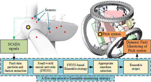
Consequently, a five-step selective ensemble strategy for dynamic fault monitoring of a pitch system is proposed. Taking the first step, the fault-causing data are partitioned according to the working states of the wind turbines, the Correlation Information Entropy (CIE) method is used to select correlation signals from the SCADA system and 10 indicators are designed to extract features of the partitioned data. Multiple SWNNs are established as ensemble members in the second step. During the third step, the features are randomly sampled to train the ensemble members. Regarding the fourth step, an improved global correlation method is used to select appropriate ensemble members. The selected members are fused to obtain a final result based on weighted integration approach in the fifth step. The final result is called the ensemble output. Considering testing and validation purposes, two case comparisons are used to verify the effectiveness of the proposed ensemble strategy.

The remaining Sections are organized as follows: Section 2 gives the fault analysis of the pitch system under different working states; Section 3 describes the novel selective-ensemble monitoring strategy and the entire process of its five steps; Section 4 and Section 5 give comparison examples to demonstrate the effectiveness of the proposed ensemble model. Finally, Section 6 concludes this paper.

2. Dynamic Fault Analysis of the Pitch System

To gain a proper grasp of the failure regularity, estimates from statistics provide all pitch fault information to support the establishment of the fault monitoring strategy. The pitch fault information includes fault types, the number of faults, and the working state of the wind turbine when a fault occurs. The structure of the pitch system is first given, then the pitch fault information is recorded from a real wind farm. More details about the information analysis can be seen in the following.

2.1. Pitch System

Figure 1 shows an example structure of the pitch system, where a pitch system is installed in the hub of a wind turbine. The pitch system consists of one central controller and three pitch devices (the #1, #2 and #3 pitch device). The central controller is the command center of the pitch system, which is used to control three pitch devices, respectively. Normally, three pitch devices are relatively independent and each one has its own individual actuator. The three pitch devices, in practice, usually are working synchronously, therefore, the #1 pitch device is chosen as an example to describe typical pitch control operations.

Regarding Figure 1, the #1 pitch device consists of a shaft controller, AC motor, battery, redundant encoder, and two limit switches. The AC motor executes the pitch actions after instructions are sent from the shaft controller. These actions occur in conjunction with other subsystems, such as the servo motor driver, brake resistor, gearbox, rotary photoelectric encoder, blade angle encoder, and limit switch. Electrical switch failures are the common type of faults in the pitch system due to the frequency response needed by this complex system, however, only a few electrical switch faults can be indicated by the SCADA system, most of them are unrecognizable and without any alerts.

2.2. Fault Rules

This part collects 12-month pitch fault information from 30 2 MW-wind turbines in a real wind farm. The information includes the fault types, the number of faults and the working states of the wind turbine. Usually, the operation of wind turbines can be divided into 4 working states according to the level of the wind speed [34]. Figure 2 shows an example layout of the four working states in a wind turbine. The 1st working state is the start-up and grid-connected stage of the wind turbine. Demonstrated in this state, the wind speed is so small that the pitch angle keeps to the minimum and the generator speed rises steadily. The wind turbine cuts into the 2nd working state, as the wind speed increases, to capture the maximum wind energy. The 3rd working state is the constant power control stage where the pitch system needs to constantly adjust the pitch angle to ensure that the wind turbine works at the rated power. During the 4th working state, the wind speed is too high, and the wind turbine will cut out and shut down.

Figure 2 also shows the average wind power curve of 30 2 MW-wind turbines and the fault statistics under different wind speeds. Taken from the statistical results shown in Figure 2, the distribution of pitch faults is directly related to the working states of the wind turbine. Once the working state is determined, in other words, the corresponding fault types also are determined., The random variation of wind speed, however, necessarily determines that the wind turbine must be switched frequently under different working states. It directly leads to the understanding that a certain fault easily might occur in one particular working state, while it might occur rarely in other ones, therefore, the SCADA data used to diagnose faults also need to be classified according to the working states.

The SCADA data is composed of multi-dimensional signal sources which are collected by multiple sensors. To accurately locate a fault, the most appropriate SCADA signals should be found first. The SCADA system can record more than 100 signals at the same time, and the highest recording frequency can reach 60 times per second. When all the signals are used for analysis and processing, the calculation is unimaginable. Additionally, faults cannot be accurately located, mainly due to the strong coupling between SCADA signals. When a fault occurs at a certain location, for example, multiple signals might alert at the same time. It also is found that there are very complex connections between SCADA signals and turbine components. Such connections will be reconnected with the change of working states. It is difficult to determine faults simply by analyzing the hardware structure of the wind turbines, therefore, it is important to find the correlation signals closely related to the faults, which is particularly helpful for the accurate identification of the pitch failures. A detailed explanation will be reported in the next section.

Taking the above considerations,

Table 1. Fault list.

Fault No.	Fault Name
F1	Pitch brake fuse
F2	Pitch control box connection
F3	Pitch drive error
F4	Pitch position error delay
F5	Pitch access time
F6	Pitch rationality
F7	Pitch stop time
F8	Pitch converter communication
F9	Synchronization of pitch position
F10	Fault-free

illustrates nine types of frequent faults (F1–F9) and one fault-free case (F10) which are the diagnostic targets of this paper according to the statistical analysis.

3. Selective Ensemble Monitoring Strategy Based on Small-World Neural Networks

A novel ensemble monitoring strategy is proposed to diagnose pitch faults by using multi-dimensional SCADA data. Such a strategy is a distributed diagnostic system, which takes four working states of the wind turbines as four parallel models. Each parallel model is a five-step selective ensemble model of SWNNs, in which the five steps are data partition, SWNN members’ creation, SWNN training, ensemble members’ selection, and ensemble output, respectively. It is noteworthy that, in the first step, the original SCADA data are divided into four sub-datasets according to the four working states of the wind turbine. To facilitate the description of the next steps, the architecture in the 2nd working state is selected as an example to display the proposed ensemble strategy, which is shown in Figure 3.

3.1. Data Partition

Data processing is the decisive step in ensuring that the ensemble strategy can achieve excellent results. Section 3.1.1 shows the original SCADA data is first partitioned into four subsets based on the four working states, respectively. Section 3.1.2 explains how a Correlation Information Entropy (CIE) method is used to select correlation signals that are related to the faults from the multi-dimensional SCADA signals. Section 3.1.3 discusses 10 indicators which are designed to extract fault-causing features and normal features from the correlation signals.

3.1.1. Data Classification Based on the Dynamic Working States

To establish the distributed diagnostic system, the original SCADA signals are divided into four groups based on the four working states of wind turbines. Figure 4 gives the process of the data classification, where the wind speed is the decision-maker for state transitions. The labels of 1st, 2nd, 3rd and 4th represent the four working states respectively, and C(v) is the division criterion which is calculated by Equation (1). The divided signals are used for further data processing and feature extraction, because it avoids confusion with other irrelevant data, especially at the beginning of data processing.

$$C(v)=\{\begin{array}{ll}1,& 0<v(t)<3\mathrm{m}/\mathrm{s},\\ 2,& 3\mathrm{m}/\mathrm{s}\le v(t)<12\mathrm{m}/\mathrm{s},\\ 3,& 12\mathrm{m}/\mathrm{s}\le v(t)<25\mathrm{m}/\mathrm{s},\\ 4,& 25\mathrm{m}/\mathrm{s}\le v(t)\end{array}$$

(1)

where, v(t) is the current wind speed, and C(v) is the division criterion.

3.1.2. Correlation Signals Selection under Dynamic Working States Based on CIE

Following the data partition, there are still many signals remaining and, as mentioned at the end of Section 2, not all of these signals are associated with the faults in a certain working state. It is necessary, therefore, to find the correlation signals related to the faults from the multi-dimensional SCADA signals. The Correlation Information Entropy (CIE) method is used to complete the above task.

CIE is an effective feature reduction approach. It can accurately measure the correlation between multiple signals on the basis of the high reliability with low calculations. Suppose that P is the SCADA output sequences of N signals within T time. Prior to computing, each signal should be centralized and normalized to ensure that all values are in the same order of magnitude. The centralized and normalized values are obtained by Equations (2) and (3), respectively.

$${\widehat{y}}_n(t)=y_n(t)-\frac{1}{N}{\displaystyle \sum _{n=1}^N{y}_n(t)}$$

(2)

$${\overline{y}}_n(t)=\frac{{\widehat{y}}_n(t)}{\sqrt{{\displaystyle \sum _{n=1}^N{({\widehat{y}}_n(t))}^2}}}$$

(3)

P can be expressed as Equation (4):

$$P={\left\{y_n(t)\right\}}_{1\le n\le N,1\le t\le T},P\in R^{T\times N}$$

(4)

where, P is the SCADA output sequences of the n^th signal, y_n(t) is the output value of the n^th signal at time t (t = 1, 2, 3,…, T). R is a matrix of real numbers.

Subsequently, the correlation matrix Q is generated by P. It contains the correlation information between N signals, which can be expanded as Equation (5):

$$Q=P^{\mathrm{T}}P=\left[\begin{array}{cccc}1& q_{12}& \cdots & q_{1N}\\ q_{21}& 1& \cdots & q_{2N}\\ ⋮& ⋮& \ddots & ⋮\\ q_{N1}& q_{N2}& \cdots & 1\end{array}\right]=I+\tilde{R},R\in R^{N\times N}$$

(5)

where, P^T is the transposition matrix of P. q_ij (q_ij ∈ [0, 1], i ≠ j, i = 1, 2,…, n, j = 1, 2,…, n) donates the correlation degree of the i^th signal to the j^th signal. The 1 in the principal diagonal of Q represents the self-correlation coefficient of the signals. I is the autocorrelation matrix, and $\tilde{R}$ is the co-correlation matrix that implies the overlap information of all signals.

The above correlation information in the Q is the correlation degree between any two signals. Next, calculate the contribution of one signal to all signals. The ${\lambda }_i^R$, ${\lambda }_i^I$ and ${\lambda }_i^{\tilde{R}}$ denote the eigenvalues of Q, I and $\tilde{R}$, respectively. The CIE is defined as Equation (6), and its range is between [0, 1]. It is worth noting that the larger the correlation degree between signals, the smaller the corresponding CIE.

$$CIE=-{\displaystyle \sum _{i=1}^N\frac{{\lambda }_i^R}{N}{\log }_N\frac{{\lambda }_i^R}{N}}$$

(6)

To find the appropriate SCADA signals related to the pitch system, the following example lists 15 initial signals in

Table 2. Signal list.

Signal No.	Signal Name
1	Wind speed
2	Active power
3	Reactive power
4	Power factor
5	Wind direction angle
6	Generator speed
7	Generator electrical power
8	Rotor speed
9, 10, 11	Pitch angle of the 3 blades
12	Generator stator temperature
13, 14, 15	Blade root moment of the 3 blades

and uses CIE to calculate the correlation of all the signals. Additionally, the 15 initial signals are all captured from different working states and each one contains 2000 samples of normal data. Figure 5 shows the CIE results of the 15 signals for different working states:

Viewing Figure 5, select the signals with their CIEs below 0.3 as the appropriate signals in different working states. The 1st and 4th working states have no appropriate signals because the pitch system is not working and is not associated with the monitoring signals. Found in the 2nd and 3rd working states, 7 signals and 8 signals are selected as the appropriate signals respectively, where the signal numbers are 2, 3, 4, 5, 7, 8, 12 and 5, 6, 7, 9, 10, 11, 12, 15. Form these selected signals into two sets of X₂ = {2, 3, 4, 5, 7, 8, 12} and X₃ = {5, 6, 7, 9, 10, 11, 12, 15}, in which X₂ and X₃ represent the 2nd and 3rd working states, respectively. Note that the 2nd and 3rd working states will continue to be studied in the following work, while the 1st and 4th working states are beyond the scope of this paper.

3.1.3. Discretized Fault Feature Extraction

Extracting fault features from the appropriate signals mainly is to find the changing characteristics from the time series. Specifically, it is the process of using discrete values to describe a limited sequence. A sliding window is used to intercept data from the appropriate signals. The abscissa of the window is a certain period of time, and the ordinate is the value of the signal. The intercepted data is called a “run”. Each run should have a label, which is a normal label or a fault label. Moreover, 10 kinds of time-domain indicators (TDIs) are designed to calculate the features of the run. The 10 TDIs are independent but closely related, which are shown in

Table 3. 10 time-domain indicators.

TDI	Meaning	Function
$T_1=\sqrt{\frac{1}{N}{\displaystyle \sum _{i=1}^N{x}_i^2}}$	Root mean square value	The validity of data and size of the noise
$T_2=\frac{1}{N}{\displaystyle \sum _{i=1}^N{\left(x_i-\left(\frac{1}{N}{\displaystyle \sum _{i=1}^N{x}_i}\right)\right)}^2}$	Variance	Dispersion of data
$\begin{array}{c}{T}_3=\frac{1}{N}{\displaystyle \sum _{i=1}^N\frac{{\left(x_i-{\overline{x}}_i\right)}^4}{{\left((1/N){\displaystyle {\sum }_{i=1}^N{(x_i)}^2}\right)}^2}},\\ {\overline{x}}_i=\frac{1}{N}{\displaystyle \sum _{i=1}^N{x}_i}\end{array}$	Kurtosis index	Sharpness or flatness of data
$T_4=\frac{\max \left|x_i\right|}{T_1}$	Peak index	The ratio of peak to the root mean square value
$T_5=\frac{\max \left|x_i\right|}{\left(1/N\right){\displaystyle {\sum }_{i=1}^N\left|x_i\right|}}$	Impulse index	Degree of data mutation
$T_6=\max \left\{x_i\right\}-\min \left\{x_i\right\}$	Peak to peak value	Mutation degree of the peak value
$T_7={\left(\frac{1}{N}{\displaystyle \sum _{i=1}^N\left(\sqrt{\left|x_i\right|}\right)}\right)}^2$	Square root amplitude	Amplitude variation of data
$T_8=\frac{1}{N}{\displaystyle \sum _{i=1}^N\left|x_i\right|}$	Average amplitude	Amplitude size of data
$T_9=\frac{T_1}{T_8}$	Waveform index	Waveform Amplitude of Data
$T_{10}=\frac{\max \left|x_i\right|}{T_8}$	Abundance index	Proportion of peak data in magnitude

. Actually, the runs with normal labels are the vast majority, and the runs with fault labels are the minority. This imbalanced distribution is undoubtedly counterproductive to further classification. A combination method combining over-sampling and under-sampling [33] is used in this case to expand the number of fault runs.

According to the correlation signals selection in Section 3.1.2, the signals of X₂ = {2, 3, 4, 5, 7, 8, 12} and X₃ = {5, 6, 7, 9, 10, 11, 12, 15} are selected as the appropriate signals for future diagnosing of the pitch failures. Taking the 2nd working state as an example, the process of discretizing feature extraction for the seven signals in X₂ is described as follows:

(1)

Define a new dataset X_t, including the X₂ = {2, 3, 4, 5, 7, 8, 12} and the label set of yⁿ(F_i).

$$X_t=\left\{x^n\left(t\right)\right\},n=2,3,4,5,7,8,12$$

(7)

$$x^n(t)=\left[x^n\left(1\right),x^n\left(2\right),...,x^n\left(t\right),y^n(F_i)\right]$$

(8)

where, t is the sampling size; n is the n^th signal, which is shown in Table 2. xⁿ(t) represents the tth value in the nth signal. yⁿ(F_i) is the label information, F_i is the fault types which are shown in Table 1.

(2)

Calculate the features of the signals based on the 10 TDIs separately, then combine the features to obtain a simplified discrete data matrix of X_n(II), which is defined as Equation (9).

(3)

Repeating the above two steps, the feature matrix of the 3rd working state can be calculated simultaneously. The discrete data matrix X_n(III) is described in Equation (10).

$$X_n(\mathrm{II})={\left[\begin{array}{cccc}{T}_1^2& T_2^2& \cdots & T_{10}^2\\ T_1^3& T_2^3& \cdots & T_{10}^3\\ ⋮& ⋮& \ddots & ⋮\\ T_1^{12}& T_2^{12}& \cdots & T_{10}^{12}\end{array}\begin{array}{c}{y}^2(F_i)\\ y^3(F_i)\\ ⋮\\ y^{12}(F_i)\end{array}\right]}_{7\times 11}$$

(9)

$$X_n(\mathrm{III})={\left[\begin{array}{cccc}{T}_1^5& T_2^5& \cdots & T_{10}^5\\ T_1^6& T_2^6& \cdots & T_{10}^6\\ ⋮& ⋮& \ddots & ⋮\\ T_1^{15}& T_2^{15}& \cdots & T_{10}^{15}\end{array}\begin{array}{c}{y}^5(F_i)\\ y^6(F_i)\\ ⋮\\ y^{15}(F_i)\end{array}\right]}_{8\times 11}$$

(10)

Considering X_n(II) and X_n(III), n represents the n^th signal in X₂ and X₃, respectively. The row vector represents the feature vector of the n^th signal, including 10 TDI values and a label value. The column vector represents all correlation signals information for the 2nd and 3rd states. Specifically, there are 70 TDIs and 7 label values in the 2nd working state, 80 TDIs and 8 label values in the 3rd working state. These TDIs and label values will be used to train SWNNs.

3.2. SWNN Members Creation

Generally, if the ensemble members are accurate and diverse, the ensemble model will be more accurate than any of its individual members [28], however, for neural network ensemble members, one drawback is that the initial situations almost determine the effect of the network. Such situations include initial parameters, training data, topology, and the learning process. Fortunately, SWNNs have been optimized in these initial situations and are well suited to be the ensemble members.

The SWNN is a middle ground neural network between regularity and disorder networks [9,35]. The probability p (0 < p <1) is used to probe the intermediate region. When p = 0 or p = 1, the SWNN are completely regular or completely random. While p increases from 0 to 1, the SWNN becomes increasingly disordered and all connections between neurons are rewired randomly. Additionally, once the number of input, output and hidden layer neurons of the network are determined, there will be a definite value of p to enable the whole network to achieve the highest clustering with the shortest characteristic path length. Quite the opposite, the SWNN also can randomly reconstruct diverse networks with different structures under the same value of probability p. Compared with the traditional neural networks, the SWNN easily can obtain various network structures by modifying p values rather than setting a large number of initial values or changing the number of neurons or layers.

The SWNN’s structure, topology and the detailed training formulas are based on the existing study [9]. Figure 6 shows the example SWNN structure of the ensemble model in the 2nd working state, where the red thick lines are the rewiring edge, and the dashed lines are the rewired edges. The detailed parameters of the SWNN will be set in Section 4.

When constructing the SWNN ensemble members for the 2nd working state, the number of input neurons is 70, which matches 70 TDIs in Equation (9). Three hidden layers are selected with 70 hidden neurons in each layer, and the activation function is a Logistic function. The number of output neurons is 10, representing 10 kinds of fault labels in Equation (9). Similarly, when constructing the SWNN ensemble members for the 3rd working state, the number of input hidden neurons are 80 to correspond the 80 TDIs in Equation (10). The training process of the SWNN will now be introduced.

3.3. SWNN Training

The SWNN ensemble members will be trained using different datasets. SWNN is a multi-layer forward neural network, which is trained by leaping forward-propagation and backward-propagation. Equation (11) shows the weight matrix of the SWNN, where the values on the diagonal line represent the weights of the regular network, while those not on the diagonal line represent the weights of random reconnection. The reconnection weights will determine the way of propagation, where Equation (11) gives the matrix space:

$$W=\left[\begin{array}{ccccc}0& 0& \cdots & 0& 0\\ 0& W_{23}& \cdots & W_{2(w-1)}& W_{1(w)}\\ ⋮& ⋮& \ddots & ⋮& ⋮\\ 0& 0& 0& W_{(w-2)(w-1)}& W_{(w-1)w}\\ 0& 0& 0& 0& W_{(w-1)w}\end{array}\right]$$

(11)

During the forward-propagation stage, suppose that P samples are given to the input layer of the SWNN, and the network outputs are obtained based on the weight vector W. The purpose is to minimize the error function E_total that is defined as:

$$E_{\mathrm{total}}=\frac{1}{2}{\displaystyle \sum _{s=1}^P{\left|Y_s-V_s\right|}^2}$$

(12)

where, Y_s is the actual output and V_s is a desired one.

During the back-propagation stage, the gradient descent method is used to obtain the optimal solutions. The direction and magnitude change $\mathsf{\Delta }{w}_{ij}$ can be computed as:

$$\mathsf{\Delta }{w}_{ij}=-\frac{\partial E_{total}}{\partial w_{ij}}$$

(13)

Each SWNN is trained by different datasets for training the ensemble members. Such datasets will be explained in the Experimental validation section. The above two stages are executed during each iteration of the back-propagation algorithm until E_total converges.

3.4. Selecting Appropriate Ensemble Members

Following training, each individual SWNN member has generated its own result, however, if there are a great number of individual members, a subset of representatives to improve ensemble efficiency needs to be selected. Existing research has proven that the selective ensemble technique can discern many members from all to achieve better classification accuracy [29]. An improved global correlation based on the Pearson Correlation Coefficient is proposed to select the appropriate SWNN members.

Suppose that there are n ensemble members (f₁, f₂,…, f_n), and each member has p forecast values. Then the total error matrix E_total can be represented by Equation (14):

$$E_{\mathrm{total}}={\left[\begin{array}{cccc}{e}_{11}& e_{12}& \cdots & e_{1n}\\ e_{21}& e_{22}& \cdots & e_{2n}\\ ⋮& ⋮& \ddots & ⋮\\ e_{p1}& e_{p2}& \cdots & e_{pn}\end{array}\right]}_{p\times n}$$

(14)

where, p = 10 represents the fault types in Table 1. e_pn is the p^th classification error of the n^th ensemble member.

According to the E_total, the mean ${\overline{e}}_i$ and the covariance V_ij are described by Equations (15) and (16), respectively.

$${\overline{e}}_i=\frac{1}{p}{\displaystyle \sum _{k=1}^p{e}_{ki}}(i=1,2,...,n)$$

(15)

$$V_{ij}=\frac{1}{p}{\displaystyle \sum _{k=1}^p\left(e_{ki}-{\overline{e}}_i\right)\left(e_{kj}-{\overline{e}}_j\right)}(i,j=1,2,...,n)$$

(16)

where, i and j (i, j = 1, 2,…, n) represent the i^th ensemble member f_i and the j^th ensemble member f_j.

Then, the correlation matrix R can be calculated by Equation (17):

$$R=\left(r_{ij}\right),r_{ij}=\frac{V_{ij}}{\sqrt{V_{ii}{V}_{jj}}}(i,j=1,2,...,n)$$

(17)

where, r_ij is the correlation coefficient that describes the degree of correlation between f_i and f_j. V_ii and V_jj are the variances of the two members, which comes from the autocorrelation coefficient r_ii = 1 and r_jj = 1 (i, j = 1, 2,…, n).

Further extended to calculate the global correlation, let ρ_fi denote the correlation between f_i and (f₁, f₂,…, f_i-1, f_i+1,…, f_n). R is a symmetric matrix whose expansion is shown in Equation (18):

$$R={\left[\begin{array}{ccccc}1& r_{12}& r_{13}& \cdots & r_{1j}\\ r_{12}& 1& r_{23}& \cdots & r_{2j}\\ r_{13}& r_{23}& 1& \ddots & ⋮\\ ⋮& ⋮& \ddots & \ddots & r_{ij}\\ r_{1j}& r_{2j}& \cdots & r_{ij}& 1\end{array}\right]}_{n\times n}$$

(18)

Subsequently, the correlation matrix R is represented by a block matrix as shown in Equation (19):

$$R\to \left[\begin{array}{cc}{R}_{-i}& r_i\\ r_i^T& 1\end{array}\right]$$

(19)

where, R_−i denotes the correlation matrix of lacking member f_i, and the transformation of R is shown in Figure 7:

Then, the plural-correlation coefficient can be calculated by Equation (20):

$${\rho }_i^2=r_i^T{R}_{-i}{r}_i(i=1,2,...,n)$$

(20)

Regarding a pre-specified threshold θ, if ${\rho }_i^2<\theta$, the member f_i is removed from the member group, otherwise, the member f_i is retained. The procedure is shown in Figure 8. Additionally, the retained members can be re-selected by repeating the process until more satisfied members are obtained.

3.5. Integrating the Multiple Members into an Ensemble Output

During the previous steps, several appropriate ensemble members of SWNN have been selected. Regarding the subsequent task, a final decision value is obtained by combining the results of the selected members based on the weighted integration method.

Suppose that there are m members retained, the outputs of the members could construct a column vector f_i according to the fault types in Table 1. f_i can be represented as Equation (21):

$$f_i={[f_i^1,f_i^2,...,f_i^k]}^{\mathrm{T}}$$

(21)

where, i = 1, 2,…, m stands for the i^th ensemble member. $f_i^k$ (k = 1, 2,…, p) is the predictive probability of the k^th output neurons in the i^th member, whose ranges is in [0, 1]. All the outputs, therefore, can be constructed by a matrix f:

$$f={\left[\begin{array}{cccc}{f}_1^1& f_2^1& \cdots & f_m^1\\ f_1^2& f_2^2& \cdots & f_m^2\\ ⋮& ⋮& \ddots & ⋮\\ f_1^p& f_2^p& \cdots & f_m^p\end{array}\right]}_{p\times m}$$

(22)

Take out the row vectors from f and one-by-one and calculate the weight values of each row. Then, the calculated weight values are reconstructed into a row vector of $\left[\begin{array}{cccc}{w}_1^k& w_2^k& \cdots & w_m^k\end{array}\right]$. Expand each w^k and construct a weight matrix w with k rows. The above processes are shown in Equations (23) and (24).

$$w_i^k=\frac{f_i^k}{{\displaystyle {\sum }_{i=1}^m{f}_i^k}}\iff \left[\begin{array}{cccc}{w}_1^k& w_2^k& \cdots & w_m^k\end{array}\right]$$

(23)

$$w={\left[\begin{array}{cccc}{w}_1^1& w_2^1& \cdots & w_m^1\\ w_1^2& w_2^2& \cdots & w_m^2\\ ⋮& ⋮& \ddots & ⋮\\ w_1^k& w_2^k& \cdots & w_m^k\end{array}\right]}_{k\times m}$$

(24)

Combine the w and f to calculate the ensemble outputs of F with the results obtained by Equations (25) and (26).

$$F=\left[\begin{array}{cccc}{f}^1& f^2& \cdots & f^k\begin{array}{cc}\cdots & f^p\end{array}\end{array}\right]$$

(25)

$$f^k={\left[f\right]}^k\times {\left[w^{\mathrm{T}}\right]}^k$$

(26)

where, $f^k$ (k = 1, 2,…, p) is the integrated probability of the k^th classification, whose ranges also are in [0, 1]. Set a threshold σ = 0.5. When $f^k\ge \sigma$, let $f^k=1$. When $f^k<\sigma$, let $f^k=0$.

To summarize, the multistage reliability-based SWNN ensemble model can be concluded in the following steps:

(1)

Pretreat the original SCADA data and extract its features to construct n training datasets, TR₁, TR₂,…, TR_n.

(2)

Train n SWNNs ensemble members with n training datasets.

(3)

Select m appropriate members based on a weighted integration method.

(4)

Fuse multiple SWNN members’ outputs into an aggregated value.

4. Experimental Validation

Actual data is used to train the ensemble model of SWNN and then applied to detect nine kinds of the abrupt and incipient faults. The training data is originated from the SCADA systems of 30 2MW-wind turbines in a wind farm for one year.

4.1. Case Preparation

Thirty SWNN members are established, respectively, for the 2nd and 3rd working states of the wind turbines, and their parameters are as shown in

Table 4. Structure information of SWNN members.

Working State	Ensemble Members	Input Neurons	Hidden Neurons ✕ Layers	Output Neurons	Probability p	Reconnection Number
2nd	30	70	70 ✕ 3	10	0.08	1232
3rd	30	80	80 ✕ 3	10	0.08	1600

:

Notably, for meeting the reliable performance, 26,000 runs of time-series datasets were captured to collect the training (TR), validation (VA) and testing (TE) data. Each run contains 3600 consecutive samples, whose sampling time is 1 second. The three types of data are distributed in accordance with the following principles:

(1)

The TE data should not overlap with others, so 6000 runs were selected at first for the final test of the SWNN members.

(2)

The remaining 20,000 runs were divided into 90% TR data and 10% VA data, using a bootstrap sampling method, and there were 12,640 runs and 7360 runs, respectively.

(3)

The abnormal runs will account for one tenth of the TR, VA and TE data respectively, and the abnormal runs also need to be allocated averagely in the TR, VA, and TE data.

(4)

Repeat sampling 30 times to get 30 groups’ datasets for each working state, then the 30 groups’ datasets are used to train the 30 SWNN members, respectively.

Table 5. Data distribution of time-series runs in Group 1.

Working State	Data	Runs
		F1	F2	F3	F4	F5	F6	F7	F8	F9	F10	Total
2nd	TR	154	139	150	134	143	141	139	145	128	11,367	12,640
	VA	84	70	74	85	91	84	83	78	80	6631	7360
	TE	67	65	68	72	71	61	79	52	68	5397	6000
3rd	TR	140	142	133	145	151	128	135	142	140	11,384	12,640
	VA	80	83	84	71	74	93	86	80	79	6630	7360
	TE	63	70	71	68	61	65	72	57	79	5394	6000

shows an example data distribution in Group 1 for the 2nd and 3rd working states, in which the F1–F9 are the labels of the 9 fault types, and F10 is the label of the fault-free.

4.2. Error Analysis

Subsequent to training the SWNN members, Figure 9 gives the calculation results of the Normalized Global Correlation (NGC) for a total 60 SWNN members, in which Figure 9a,b represent the 2nd and 3rd working state, respectively. Ranking the testing values of NGC, the first 8 SWNN members are selected to construct a selective ensemble model for each working state. Furthermore, the selective ensemble model is used to predict and classify 10 types of faults, and the fault prediction distribution and the classification rate are shown in Figure 10 and

Table 6. Correct classification rate of selective members.

Working State	Data Case	Ensemble Members’ Number								Ensemble Rate
		1	2	3	4	5	6	7	8
2nd	TR	98.45%	98.05%	97.9%	97.5%	97.5%	97.39%	97.34%	97.28%	98.20%
	TE	92.70%	90.78%	95.26%	93.51%	93.35%	92.88%	92.51%	92.41%	93.84%
3rd	TR	98.71%	98.58%	98.44%	98.44%	98.39%	98.34%	98.31%	98.26%	98.63%
	TE	94.47%	93.85%	93.22%	93.22%	92.87%	92.64%	93.12%	92.55%	94.11%

, respectively.

Figure 10 illustrates, the fifth fault has the lowest accuracy while among the other types of faults there are also many cases of misclassification and missed judgment. Table 6 shows, in the 2nd and 3rd working states, the training accuracy and testing accuracy of the 8 SWNN classifiers are over 97% and 92%, respectively. It can be illustrated that the SWNNs are close to each other in classification accuracy, which benefits from its special network structure, i.e., the homogeneous but structurally stochastic structure. Additionally, the SWNN ensemble model has a higher accuracy rate (93.8%) than that of the SWNN members. It proves that SWNN is very suitable as the ensemble members, and the proposed selective SWNN ensemble model can detect nine pitch faults effectively.

5. Comparison Validation

The proposed selective SWNN ensemble model is compared with three existing methods for online fault detection. The false alarm rate (FAR), the missed fault rate (MFR), and the mean fault diagnosis delay (MFD) are used as the evaluation indices to evaluate the performance of these models.

5.1. Comparison Approaches

Three comparison approaches are TRSWA-BP Neural Network (TRSWA-NN) [12], SWPSO-Support Vector Regression (SWPSO-SVR) [36] and SWPSO learning vector quantization (SWPSO-LVQ), which are presented briefly. They have shown good performance in wind power prediction and fault diagnosis of wind turbines, which are compared based on the former captured data.

TRSWA-NN: This neural network’s learning process is based on an efficiency tabu, real-coded, small-world optimization algorithm (TRSWA), which combines EMD (empirical mode decomposition), PSR (phase space reconstruction), and EMD-based PSR to detect and isolate the faults of wind turbines.

SWPSO-SVR: This scheme uses the combination of support vector regression and small-world particle swarm optimization for fault detection and isolation in wind turbines.

SWPSO-LVQ: This scheme combines the LVQ network based on the small-world particle swarm optimization for detection and isolation, which has a good performance for all of the faults.

5.2. Evaluation Indices

The evaluation indices contain false alarm rate (FAR), missed fault rate (MFR) and mean fault diagnosis delay (MFD). The three indices are calculated as follows:

$$FAR=l_{i,10}/{\displaystyle \sum _{j=1}^{10}{l}_{j,10}}$$

(27)

$$MFR={\displaystyle \sum _{j=1,i=1}^{10}{l}_{j,i}}/{\displaystyle \sum _{j=1}^{10}{l}_{j,i}}$$

(28)

$$MFD=t_{\mathrm{fault}\mathrm{occurrence}}-t_{\mathrm{fault}\mathrm{detection}/\mathrm{isolation}}$$

(29)

where, l_j,i is the number of samples from the ith class but classified to the jth class. MFD represents the delay time between the fault occurrence and fault detection/isolation.

5.3. Comparative Analysis

The same datasets above will be applied to train the three models and the proposed selective SWNN ensemble model. Monte-Carlo analysis [37] is used to calculate the indices and to test the robustness of the comparison approaches. Particularly, a rigorous test simulation based on 10,000 runs has been executed, during which realistic wind turbine uncertainties have been considered.

Table 7. Comparisons of the presented method and other approaches.

Fault Case	Index	Selective SWNN Ensemble Model	TRSWA-NN	SWPSO-SVR	SWPSO-LVQ
1	FAR	0.012	0.021	0.034	0.018
	MFR	0.009	0.019	0.048	0.013
	MFD(s)	0.08	0.12	0.02	0.11
2	FAR	0.018	0.043	0.021	0.031
	MFR	0.021	0.024	0.043	0.033
	MFD(s)	0.1	0.23	0.02	0.3
3	FAR	0.008	0.01	0.011	0.005
	MFR	0.005	0.008	0.02	0.009
	MFD(s)	0.03	0.06	0.01	0.08
4	FAR	0.037	0.042	0.113	0.068
	MFR	0.031	0.034	0.09	0.073
	MFD(s)	1.3	3.7	0.5	1.8
5	FAR	0.021	0.022	0.081	0.035
	MFR	0.017	0.026	0.09	0.01
	MFD(s)	0.13	0.11	0.02	0.15
6	FAR	0.011	0.015	0.065	0.045
	MFR	0.012	0.017	0.055	0.033
	MFD(s)	0.08	0.12	0.03	0.08
7	FAR	0.019	0.035	0.057	0.04
	MFR	0.022	0.018	0.055	0.017
	MFD(s)	0.1	2.3	0.01	0.18
8	FAR	0.08	0.062	0.153	0.091
	MFR	0.072	0.04	0.181	0.08
	MFD(s)	8.5	4.8	0.8	3.8
9	FAR	0.11	0.12	0.135	0.108
	MFR	0.067	0.094	0.19	0.124
	MFD(s)	11.8	8.3	1.5	6.9

shows the performance of the selective SWNN ensemble model against other approaches.

The results from Table 7 show the overall efficacy of the proposed ensemble SWNN model. Particularly in the neural network-based approaches of the ensemble SWNN model, TRSWA-NN and SWPSO-LVQ, it seems to achieve interesting results with quite low FAR, MFR and MRD for all the fault cases. More specifically, when identifying the first 7 faults, the maximum FAR and MFR of the ensemble model are 0.037 and 0.031, respectively, and the maximum MFD is not more than 1.3 s; while, when identifying the 8th and 9th faults, the FAR and MFR are about 0.1 and 0.08, and the minimum MFD is 8.5 s. There are many differences between the two situations, meaning that the ensemble model has good accuracy and can maintain a fast corresponding speed for diagnosing the first 7 pitch faults, but it is not ideal for the latter 2 faults. The same situation occurs in the TRSWA-NN and SWPSO-LVQ models, which can easily monitor the first 7 faults. SWPSO-SVR has a very small MFD in diagnosing all kinds of the 9 faults, however. The SWPSO-SVR has no better FAR and MFR, which means it cannot guarantee high fault recognition accuracy when dealing with multi-dimensional and large amounts of SCADA data. Conversely, compared with TRSWA-NN and SWPSO-LVQ, the selective SWNN ensemble model also shows the optimal results with smaller FAR, MFR and MFD, especially when identifying and classifying the first seven pitch faults.

6. Conclusions

Fault diagnosis of wind turbines, as a basic research project, plays a major role in today’s electricity markets. The five-step ensemble strategy proposed is a novel technique that uses the small-world neural networks as the ensemble members to improve monitoring reliability and classification accuracy. Compared to the conventional methods, the proposed method can be summarized as follows:

(1)

The proposed selective SWNN ensemble strategy provides a comprehensive monitoring mechanism for most fault types under different working states of the wind turbines.

(2)

The proposed selective SWNN ensemble strategy decomposes the dynamic monitoring into four distributed ensemble models, and each model contains multiple SWNNs to selectively output multiple judgment results. These results can be coordinated to provide consistent fault classifications at a fixed prediction horizon. The classification performance is effective and accurate. Specifically, the proposed method under different working states shows an average training accuracy and testing accuracy of over 97% and 92%, respectively, when detecting the most pitch failures.

(3)

The proposed selective SWNN ensemble strategy reveals stronger adaptability and sensitivity than that of the single SWNN, especially when classifying and identifying the abrupt and incipient faults, with a higher accuracy rate of over 93.8%. Additionally, it is able to use a short delay time while achieving a lower false alarm rate and lower missed fault rate than the conventional models.

Future works focus on: (1) Regarding data processing, the ratio of normal samples to abnormal samples needs to be studied. Such ratio will play a decisive role in the final classification results. (2) Concerning terms of ensemble member optimization, a deep small-world neural network will be proposed to diagnose the fault of wind turbines. It will be compared with other deep learning algorithms, such as the Convolutional Neural Network (CNN), the Long Short-Term Memory (LSTM) and the Recurrent Neural Network (RNN).

References

1. Lin, Y.G.; Tu, T.; Liu, H.W.; Li, W. Fault analysis of wind turbines in China. Renew. Sustain. Energy Rev. 2016, 55, 482–490. [Google Scholar] [CrossRef]
2. Nandi, T.N.; Herrig, A.; Brasseur, J.G. Non-steady wind turbine response to daytime atmospheric turbulence. Phil. Trans. R. Soc. A 2017, 375, 20160103. [Google Scholar] [CrossRef] [PubMed]
3. Churchfield, M.J.; Lee, S.; Michalakes, J.; Moriarty, P.J. A numerical study of the effects of atmospheric and wake turbulence on wind turbine dynamics. J. Turbul. 2012, 13, N14. [Google Scholar] [CrossRef]
4. Laks, J.; Pao, L.; Wright, A.; Kelley, N.; Jonkman, B. The use of preview wind measurements for blade pitch control. Mechatronics 2011, 21, 668–681. [Google Scholar] [CrossRef]
5. Kelley, N.; Hand, M.; Larwood, S.; McKenna, E. The NREL large-scale turbine inflow and response experiment- Preliminary results. In Proceedings of the 2002 ASME Wind Energy Symposium, Reno, NV, USA, 14–17 January 2002; pp. 412–426. [Google Scholar]
6. Jiang, Y.; Yin, S.; Kaynak, O. Data-driven monitoring and safety control of industrial cyber-physical systems: Basics and beyond. IEEE Access 2018, 6, 47374–47384. [Google Scholar] [CrossRef]
7. Rahimilarki, R.; Gao, Z.W.; Zhang, A.H.; Richard, J.B. Robust neural network fault estimation approach for nonlinear dynamic systems with applications to wind turbine systems. IEEE Trans. Ind. Inf. 2019, 18. [Google Scholar] [CrossRef]
8. Marugán, A.P.; Márquez, F.P.G.; Perez, J.M.P.; Ruiz-Hernández, D. A survey of artificial neural network in wind energy systems. Appl. Energy 2018, 228, 1822–1836. [Google Scholar] [CrossRef] [Green Version]
9. Wang, S.X.; Li, M.; Zhao, L.; Jin, C. Short-term wind power prediction based on improved small-world neural network. Neural Comput. Appl. 2018, 29, 1–13. [Google Scholar] [CrossRef]
10. Marugán, A.P.; Chacón, A.M.P.; Márquez, F.P.G. Reliability analysis of detecting false alarms that employ neural networks: A real case study on wind turbines. Reliab. Eng. Syst. Saf. 2019, 191, 106574. [Google Scholar] [CrossRef] [Green Version]
11. Pelletier, F.; Masson, C.; Tahan, A. Wind turbine power curve modelling using artificial neural network. Renew. Energy 2016, 89, 207–214. [Google Scholar] [CrossRef]
12. Wang, S.X.; Zhao, X.; Li, M.; Wang, H. TRSWA-BP neural network for dynamic wind power forecasting based on entropy evaluation. Entropy 2018, 20, 283. [Google Scholar] [CrossRef]
13. Cheng, F.Z.; Peng, Y.Y.; Qu, L.Y.; Qian, W. Current-based fault detection and identification for wind turbine drivetrain gearboxes. IEEE Trans. Ind. Appl. 2017, 53, 878–887. [Google Scholar] [CrossRef]
14. Stetco, A.; Dinmohammadi, F.; Zhao, X.Y.; Robu, V.; Flynn, D.; Barnes, M.; Keane, J.; Nenadic, G. Machine learning methods for wind turbine condition monitoring: A review. Renew. Energy 2019, 133, 620–635. [Google Scholar] [CrossRef]
15. Cheng, F.Z.; Wang, J.; Qu, L.Y.; Qian, W. Rotor current-based fault diagnosis for DFIG wind turbine drivetrain gearboxes using frequency analysis and a deep classifier. IEEE Trans. Ind. Appl. 2018, 54, 1062–1071. [Google Scholar] [CrossRef]
16. Zhao, H.S.; Liu, H.H.; Hu, W.J.; Yan, X.H. Anomaly detection and fault analysis of wind turbine components based on deep learning network. Renew. Energy 2018, 127, 825–834. [Google Scholar] [CrossRef]
17. Teng, W.; Cheng, H.; Ding, X.; Liu, Y.B.; Ma, Z.Y.; Mu, H.H. DNN-based approach for fault detection in a direct drive wind turbine. IET Renew. Power Gener. 2018, 12, 1164–1171. [Google Scholar] [CrossRef]
18. Grimshaw, S. An Introduction to the Bootstrap. Technometrics 2012, 37, 340–341. [Google Scholar] [CrossRef]
19. Breiman, L. Bagging predictors. Mach. Learn. 1996, 24, 123–140. [Google Scholar] [CrossRef] [Green Version]
20. Freund, Y. Boosting a weak algorithm by majority. Inf. Comput. 1995, 121, 256–285. [Google Scholar] [CrossRef]
21. Liu, Y.; Yao, X. Ensemble learning via negative correlation. Neural Netw. 1999, 12, 1399–1404. [Google Scholar] [CrossRef]
22. Qin, S.; Wang, K.; Ma, X.; Wang, W.; Li, M. Ensemble learning-based wind turbine fault prediction method with adaptive feature selection. In Proceedings of the International Conference of Pioneering Computer Scientists, Engineers and Educators, Changsha, China, 22–24 September 2017; pp. 572–582. [Google Scholar]
23. Sollich, P.; Krogh, A. Learning with ensembles: How over-fitting can be useful. In Advances in Neural Information Processing Systems 8; Touretzky, D.S., Mozer, M.C., Hasselmo, M.E., Eds.; MIT Press: Denver, CO, USA; Cambridge, MA, USA, 1996; pp. 190–196. [Google Scholar]
24. Schapire, R.E. The strength of weak learnability. Mach. Learn. 1990, 5, 197–227. [Google Scholar] [CrossRef] [Green Version]
25. Pashazadeh, V.; Salmasi, F.R.; Araabi, B.N. Data driven sensor and actuator fault detection and isolation in wind turbine using classifier fusion. Renew. Energy 2018, 116, 99–106. [Google Scholar] [CrossRef]
26. Dey, S.; Pisu, P.; Ayalew, B. A Comparative study of three fault diagnosis schemes for wind turbines. IEEE Trans. Control Syst. Technol. 2015, 23, 1853–1868. [Google Scholar] [CrossRef]
27. Hornik, K.; Stinchocombe, M.; White, H. Multilayer feedforward networks are universal approximators. Neural Netw. 1989, 2, 359–366. [Google Scholar] [CrossRef]
28. Hansen, L.K.; Salamon, P. Neural network ensembles. IEEE Trans. Pattern Anal. Mach. Intell. 1990, 12, 993–1001. [Google Scholar] [CrossRef] [Green Version]
29. Zhou, Z.H.; Wu, J.X.; Tang, W. Ensembling neural networks: Many could be better than all. Artif. Intell. 2002, 137, 239–263. [Google Scholar] [CrossRef] [Green Version]
30. Morelli, L.G.; Abramson, G.; Kuperman, M.N. Associative memory on a small-world neural network. Eur. Phys. J. B-Condens. Matter Complex Syst. 2004, 38, 495–500. [Google Scholar] [CrossRef] [Green Version]
31. Zhao, X.; Wang, S.X. Convergence analysis of the tabu-based real-coded small-world optimization algorithm. Eng. Optim. 2014, 46, 465–486. [Google Scholar] [CrossRef]
32. Suen, C.Y.; Lam, L. Multiple classifier combination methodologies for different output levels. Lect. Notes Comput. Sci. 2000, 1857, 52–66. [Google Scholar]
33. Wu, Z.; Lin, W.; Ji, Y. An integrated ensemble learning model for imbalanced fault diagnostics and prognostics. IEEE Access 2018, 6, 8394–8402. [Google Scholar] [CrossRef]
34. Wang, N. Advanced wind turbine control. Adv. Wind Turbine Technol. 2018, 5, 281–297. [Google Scholar]
35. Watts, D.J.; Strogatz, S.H. Collective dynamics of ‘small-world’ networks. Nature 1998, 393, 440–442. [Google Scholar] [CrossRef] [PubMed]
36. Wang, S.X.; Li, M.; Tian, T.T.; Zhang, J.H. Evaluation and prediction of operation status for pitch system based on SCADA data. In Proceedings of the 2017 Chinese Automation Congress (CAC), Jinan, China, 20–22 October 2017; pp. 3327–3332. [Google Scholar]
37. Simani, S.; Castaldi, P.; Farsoni, S. Data-driven fault diagnosis of a wind farm benchmark model. Energies 2017, 10, 866. [Google Scholar] [CrossRef]
Figure 1. The structure of the pitch system in a wind turbine.
Energies 12 03256 g001
Figure 2. State partition and fault statistics for the 30 2 MW wind turbines.
Energies 12 03256 g002
Figure 3. A five-step selective ensemble strategy for dynamic fault monitoring of pitch system in the 2nd working state.
Energies 12 03256 g003
Figure 4. Data classification according to the working states.
Energies 12 03256 g004
Figure 5. The Correlation Information Entropy (CIE) results of 15 initial signals.
Energies 12 03256 g005
Figure 6. SWNN ensemble members in the 2nd working state.
Energies 12 03256 g006
Figure 7. Transformation of correlation matrix R.
Energies 12 03256 g007
Figure 8. Procedure for selecting ensemble members.
Energies 12 03256 g008
Figure 9. Normalized Global Correlation (NGC) of the ensemble members.
Energies 12 03256 g009
Figure 10. Fault prediction distribution of selective ensemble model.
Energies 12 03256 g010