Fast Torque Computation of Hysteresis Motors and Clutches Using Magneto-static Finite Element Simulation


Abstract
:1. Introduction
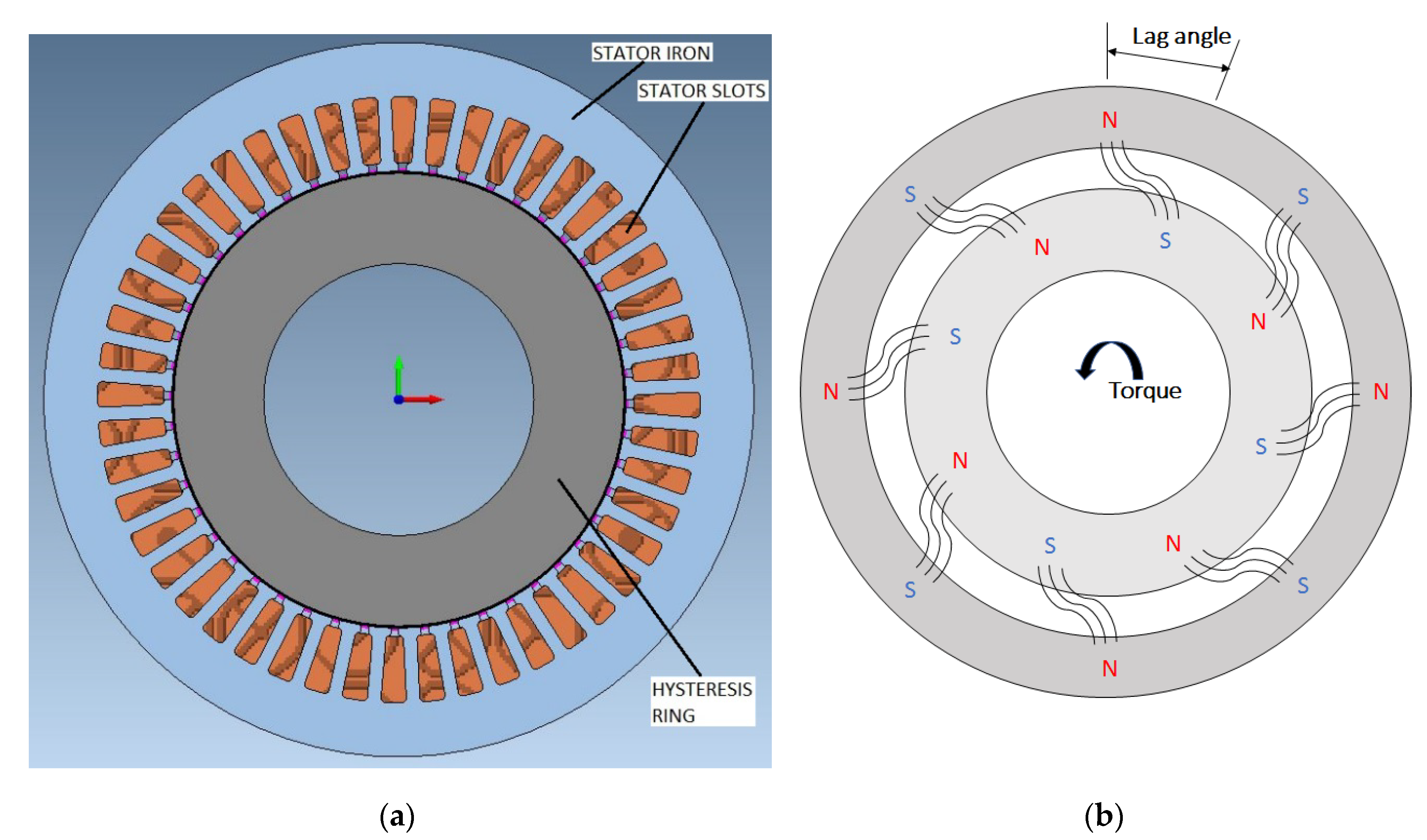
2. Working Principle
3. Analytical Approach
4. Finite Element Analysis
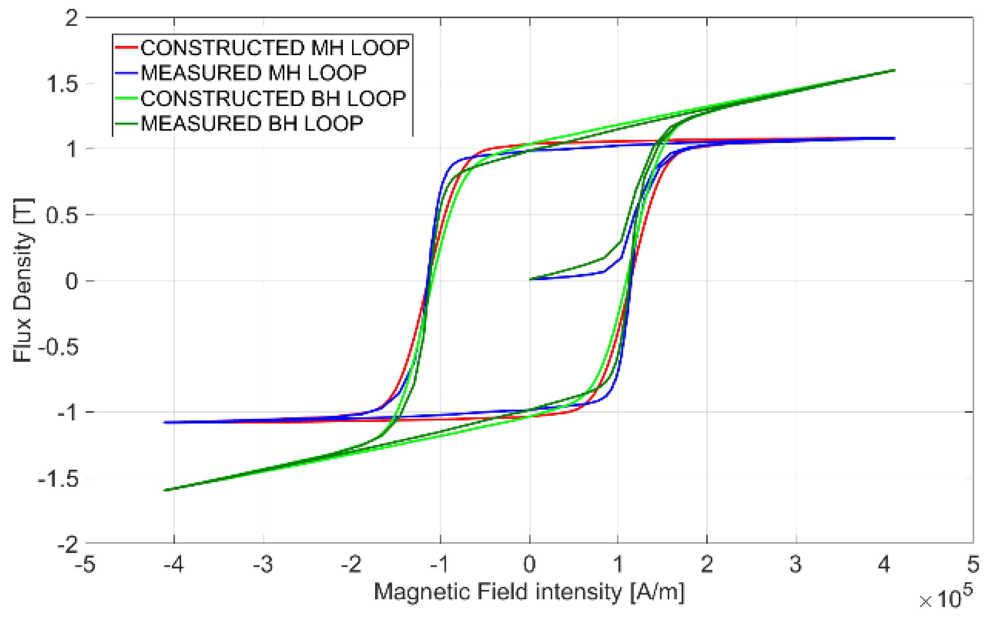
4.1. Hysteresis Modeling
4.2. Fea Approach
- Finite element analysis with initial permeability and initial .
- Calculation of Btan for each ring element and evaluation of the maximum of .
- Evaluation of the actual value of H from the hysteresis model.
- Computation of the new inputs for the finite element analysis.
5. Proposed Method
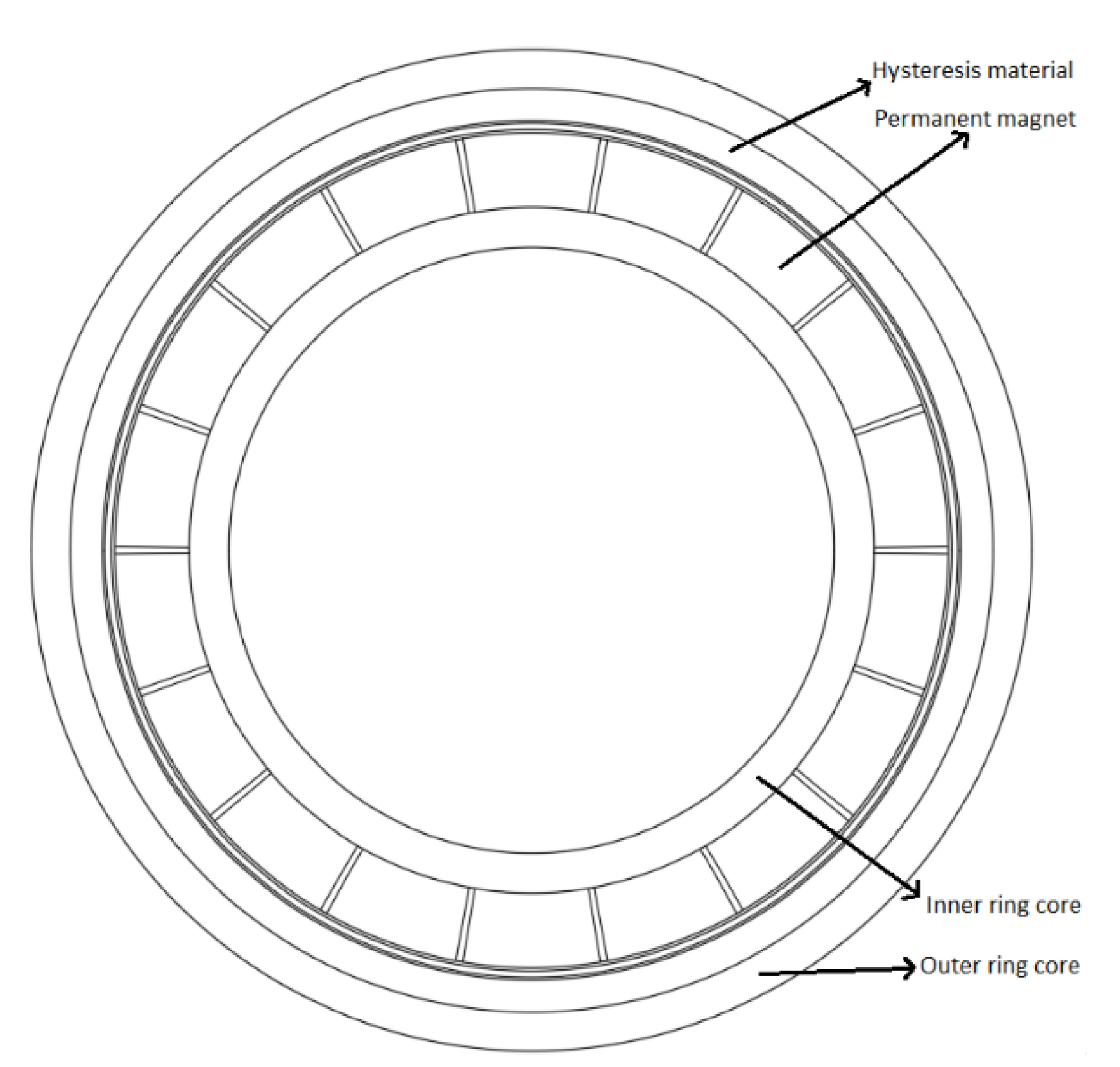
6. Case of Study
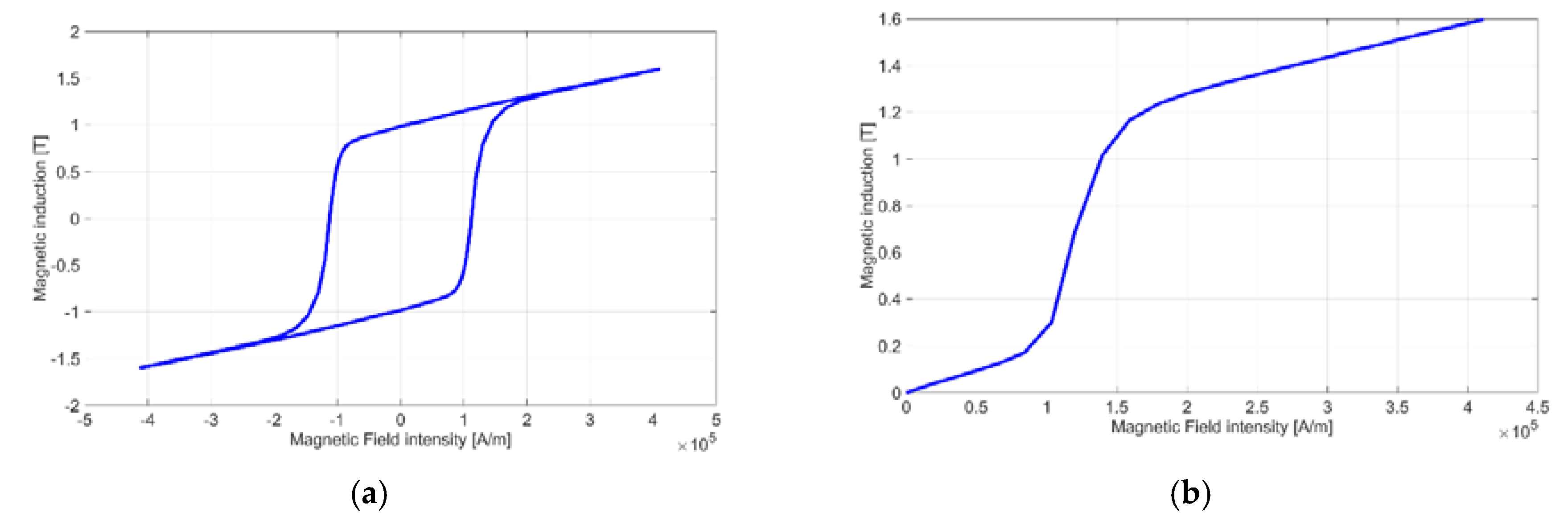
- the normal magnetization curve
- the value of the intrinsic coercive field
- the value of the residual flux density (optional)
7. Conclusions
Author Contributions
Funding
Conflicts of Interest
References
- Mayr, A.; Weigelt, M.; von Lindenfels, J.; Seefried, J.; Ziegler, M.; Mahr, A.; Urban, N.; Kühl, A.; Hüttel, F.; Franke, J. Electric Motor Production 4.0—Application Potentials of Industry 4.0 Technologies in the Manufacturing of Electric Motors. In Proceedings of the 8th International Electric Drives Production Conference (EDPC), Schweinfurt, Germany, 4–5 December 2018; pp. 1–13. [Google Scholar]
- Tsai, W.-H. Green Production Planning and Control for the Textile Industry by Using Mathematical Programming and Industry 4.0 Techniques. Energies 2018, 11, 2072. [Google Scholar] [CrossRef]
- Steinmetz, C.P. Theory and Calculation of Alternating Current Phenomena; McGraw Hill Book Company, Inc.: New York, NY, USA, 1908; p. 122. [Google Scholar]
- Parvin, F.; Nasiri-Zarandi, R.; Mirsalim, M.; Cavagnino, A. General design algorithm for a hybrid hysteresis motor based on mathematical modeling. In Proceedings of the IECON 2016-42nd Annual Conference of the IEEE Industrial Electronics Society, Florence, Italy, 23–26 October 2016; pp. 1656–1661. [Google Scholar]
- Circosta, S.; Galluzzi, R.; Bonfitto, A.; Castellanos, L.M.; Amati, N.; Tonoli, A. Modeling and Validation of the Radial Force Capability of Bearingless Hysteresis Drives. Actuators 2018, 7, 69. [Google Scholar] [CrossRef]
- Galluzzi, R.; Amati, N.; Tonoli, A. Modeling, Design and Validation of Magnetic Hysteresis Motors. IEEE Trans. Ind. Electron. 2019. [Google Scholar] [CrossRef]
- Roters, H.C. The hysteresis motor-advances whick permit economical fractional horsepower ratings. Trans. Am. Inst. Electr. Eng. 1947, 66, 1419–1430. [Google Scholar] [CrossRef]
- Teare, B.R. Theory of hysteresis-motor torque. Electr. Eng. 1940, 59, 907–912. [Google Scholar] [CrossRef]
- Copeland, M.A.; Slemon, G.R. An analysis of the hysteresis motor I-analysis of the idealized machine. IEEE Trans. Power Appar. Syst. 1963, 82, 34–42. [Google Scholar] [CrossRef]
- Kim, H.K.; Hong, S.K.; Jung, H.K. Analysis of hysteresis motor using finite element method and magnetization-dependent model. IEEE Trans. Magn. 2000, 36, 685–688. [Google Scholar]
- Nasiri-Zarandi, R.; Mirsalim, M. Finite-element analysis of an axial flux hysteresis motor based on a complex permeability concept considering the saturation of the hysteresis loop. IEEE Trans. Ind. Appl. 2015, 52, 1390–1397. [Google Scholar]
- Bi, S. Charakterisieren und modellieren der ferromagnetischen hysterese. Ph.D. Thesis, Friedrich-Alexander-Universität Erlangen-Nürnberg, Erlangen-Nürnberg, Germany, 2014. [Google Scholar]
- Noh, M.; Gruber, W.; Trumper, D.L. Hysteresis Bearingless Slice Motors with Homopolar Flux-Biasing. IEEE/ASME Trans. Mech. 2017, 22, 2308–2318. [Google Scholar] [CrossRef] [PubMed]
- Nitao, J.J.; Scharlemann, E.T.; Kirkendall, B.A. Equivalent Circuit Modeling of Hysteresis Motors; No. LLNL-TR-416493; Lawrence Livermore National Lab (LLNL): Livermore, CA, USA, 2009.
- Canova, A.; Cavalli, F. Design procedure for hysteresis couplers. IEEE Trans. Magn. 2008, 44, 2381–2395. [Google Scholar] [CrossRef]
- Jiles, D.C.; Thoelke, J.B.; Devine, M.K. Numerical determination of hysteresis parameters for the modeling of magnetic properties using the theory of ferromagnetic hysteresis. IEEE Trans. Magn. 1992, 28, 27–35. [Google Scholar] [CrossRef]
- Bertotti, G. Hysteresis in Magnetism: For Physicists, Materials Scientists, and Engineers; Academic: New York, NY, USA, 1998; pp. 433–504. [Google Scholar]
- Kim, H.S.; Hong, S.K.; Han, J.H.; Choi, D.J. Dynamic Modeling and Load Characteristics of Hysteresis Motor Using Preisach Model. In Proceedings of the 2018 21st International Conference on Electrical Machines and Systems (ICEMS), Jeju, Korea, 7–10 October 2018; pp. 560–563. [Google Scholar]
- Torre, E.D. Existence of magnetization-dependent Preisach models. IEEE Trans. Magn. 1991, 27, 3697–3699. [Google Scholar] [CrossRef]
- Lin, D.; Zhou, P.; Lu, C.; Chen, N.; Rosu, M. Construction of magnetic hysteresis loops and its applications in parameter identification for hysteresis models. In Proceedings of the 2014 International Conference on Electrical Machines (ICEM), Berlin, Germany, 2–5 September 2014; pp. 1050–1055. [Google Scholar]
- Lin, D.; Zhou, P.; Bergqvist, A. Improved vector play model and parameter identification for magnetic hysteresis materials. IEEE Trans. Magn. 2014, 50, 357–360. [Google Scholar] [CrossRef]
- Repetto, M.; Uzunov, P. Analysis of hysteresis motor starting torque using finite element method and scalar static hysteresis model. IEEE Trans. Magn. 2013, 49, 2405–2408. [Google Scholar] [CrossRef]
- Finite Element Method Magnetics. Available online: http://www.femm.info (accessed on 3 July 2019).


| Type of Ferromagnetic Material | Coercive Field [A/m] |
|---|---|
| Soft | <1000 |
| Semi-hard | <50,000 |
| Hard | >50,000 |
| Analytical Approach | Hysteresis Loop Shape | Dependence of the Coercive Field by the Saturation Level | Type of Machine | Accuracy |
|---|---|---|---|---|
| [8] | Inclined ellipse | Yes | Circumferential | ++ |
| [9] | Parallelogram | No | Radial | + |
| Method | Accuracy of the Model | Computational Cost | Ease of Implementation |
|---|---|---|---|
| [10] | ++ | +++ | +++ |
| [11] | + | + | + |
| [22] | + | + | + |
| Parameter | Value | Units |
|---|---|---|
| Number of pole pairs | 9 | \ |
| Inner diameter | 46.8 | mm |
| Outer diameter | 77.4 | mm |
| Inner core radial thickness | 3.1 | mm |
| Outer core radial thickness | 3 | mm |
| Permanent Magnets radial thickness | 5.75 | mm |
| Hysteresis region radial thickness | 2.5 | mm |
| Axial length | 27 | mm |
| Comparison Variable | Proposed Method | Transient Method |
|---|---|---|
| Mean torque [Nm] | 6.48 | 6.45 |
© 2019 by the authors. Licensee MDPI, Basel, Switzerland. This article is an open access article distributed under the terms and conditions of the Creative Commons Attribution (CC BY) license (http://creativecommons.org/licenses/by/4.0/).
Share and Cite
Gallicchio, G.; Palmieri, M.; Di Nardo, M.; Cupertino, F. Fast Torque Computation of Hysteresis Motors and Clutches Using Magneto-static Finite Element Simulation. Energies 2019, 12, 3311. https://doi.org/10.3390/en12173311
Gallicchio G, Palmieri M, Di Nardo M, Cupertino F. Fast Torque Computation of Hysteresis Motors and Clutches Using Magneto-static Finite Element Simulation. Energies. 2019; 12(17):3311. https://doi.org/10.3390/en12173311
Chicago/Turabian StyleGallicchio, Gianvito, Marco Palmieri, Mauro Di Nardo, and Francesco Cupertino. 2019. "Fast Torque Computation of Hysteresis Motors and Clutches Using Magneto-static Finite Element Simulation" Energies 12, no. 17: 3311. https://doi.org/10.3390/en12173311