Abstract
With the advance of China’s power system reform, combined heat and power (CHP) units can participate in multi-energy market. In order to maximize CHP profit in a multi-energy market, a bidding strategy for deep peak regulation auxiliary service of a CHP based on a two-stage stochastic programming risk-averse model and district heating network (DHN) energy storage was proposed. The quotation set of competitors and load uncertainty was modeled with a Latin hypercube sampling (LHS) method. A dynamic queuing method was used to clear the market for the deep peak regulation auxiliary service to determine the bidding capacities of CHPs in the electricity market and the deep peak regulation auxiliary service market, respectively. Finally, the conditional value-at-risk (CVaR) indicator is used to measure the risk brought by the system uncertainty to the CHP, and the quotation coefficient is determined after considering the expected profit and risk profit comprehensively. The results of the example show that the profits produced by simultaneous participation in both electricity market and the deep peak regulation auxiliary service market are increased by approximately 9.5% compared with the profits produced by only participation in a single market. In addition, the use of DHN energy storage led to a profit increase of approximately 4.6%. As the risk aversion coefficient increases, the expected profit will be further reduced.
1. Introduction
In the power supply structure of the Northeast China Power Grid, combined heat and power (CHP) units account for more than 60% of thermal power units. During the heating period, the CHP units at full capacity, and the condensing units (CONs) with strong deep peak regulation ability are shut down a lot, resulting in a shortage of system peaking resources. The direct cause of the shortage of peaking resources is CHP units operating on the principle of “power determined by heat”, but the root cause is that all kinds of power sources compete for power generation space, which is a problem of interest distribution. To solve this problem, a peak regulation ancillary service market for was established for the Northeast China Power Grid [1]. Through market-based means, CHP units are encouraged to carry out flexible technical transformations to improve the peak regulation capacity of the units and alleviate the shortage of peak regulation resources in the system. According to statistics, in the third quarter of 2017, the peaking compensation for the peak regulation ancillary service market for the Northeast China Power Grid has exceeded $163 million. The lowest-priced service price in the peak regulation ancillary service market for the Northeast China Power Grid is $66, roughly twice the normal power generation profit of thermal power plants [1]. This means that the profits of CHP units providing deep peak regulation ancillary service are higher than the profits of electricity sales. Therefore, it is necessary to study the bidding strategy of CHP units in the deep peak regulation ancillary service market.
Regarding the related research on the deep peak regulation service participating in the power auxiliary service market, most literatures are currently studied from the perspective of maximizing the overall market profit. Moreover, at present, only condensing units have been studied to provide deep peak regulation capacity to obtain profits, and few studies have involved the situation in which CHP units provide deep peak regulation ancillary services to obtain profits. For example, in [2], from the perspective of the condensing unit, deep peak regulation ancillary service is provided to obtain the profit. The simulation example shows that the unit can obtain the maximum profit after reaching the optimal deep peak regulation point, after which, with the increase in deep peak regulation capacity, the deep peak regulation profit has gradually decreased. Liu’s research shows that the deep peak regulation cost has a great impact on the deep peak regulation profit [3]. If the bidding strategy is unreasonable, the deep peak regulation profit of the condensing unit will be lower than the basic peak regulation profit. Li [4] studied the problem of maximizing the overall profit of the deep peak regulation ancillary service market. Peng [5] studied the power generation group with wind power and CHP units as the mainstay to participate in the deep peak regulation ancillary service market on the premise of maximizing the profits of the group. However, references [4,5] only consider the peaking service of the thermal power unit demand and undertake a deep peaking cost sharing, and do not consider the provision of the deep peaking auxiliary service to obtain profits. However, the CHP unit has improved the deep peak regulation capability through the flexibility of technical transformation measures, which can provide deep peak regulation ancillary services for the market. Potential solutions for CHP units to increase flexibility include installing heat pumps [6,7], electric heat boilers [8,9], and equipping them with a heat storage tank [10,11], although these measures may not be employed because they require excessive capital investment. At the same time, the district heating network (DHN) provides additional flexibility for CHP unit operation. A DHN consists of insulated pipelines with large heat storage capacity, which can improve the flexibility of CHP units. As a city infrastructure, DHNs already exist in urban areas without additional investment. DHNs can break the power and heat coupling without additional investment [12,13]. In addition to the large scale DHN control method modeling mentioned above, [14,15,16] studied the small scale DHN control method. Regardless of whether a large scale DHN or a small scale DHN is considered, both can be reduced to a similar mathematical model.
In addition, the above studies do not address the issue of electricity bidding strategy between the electricity market and the deep peak regulation ancillary service market. If the market clearing price of the deep peak regulation ancillary service market is lower than the price of the electricity market, direct sales of electricity will yield higher profits (since the electric energy spot market of the Northeast Power Grid has not been established yet, the market clearing price of the deep peaking auxiliary service market is referred to as the market clearing price). The strategy subject needs to determine the bidding generation capacity in the electricity market and the deep peak regulation ancillary service market according to the predicted market clearing price to obtain higher profits.
The settlement method of the deep peak regulation ancillary service profits is the sum of the product of the winning bidding generation capacity and the market clearing price of each level. Because market clearing prices have the characteristics of non-equilibrium mean variance, multiple seasonality, and obvious calendar effects [17], it is not easy to obtain accurate price forecasts. However, CHP still needs to estimate the price in order to make the optimal decision. Stochastic programming constructs a modeling framework for decision problems under uncertainty. In order to model a stochastic process, a limited set of scenario and their corresponding occurrence probabilities are generated for each uncertainty parameter [18]. Su [19] and Rajesh [20] studied the use of Monte Carlo simulation (MCS) to generate a set of market clearing price scenarios to represent a robust bid for price uncertainty. For the problem that the MCS has a high sampling probability around the mean and the probability of sampling at both ends is small, Gazafroudi [17] and Shi [21] proposed the use of Latin hypercube sampling (LHS) techniques to generate price and load scenarios to maintain the main features of the original probability density function. These models are expected value models and do not take into account the risk of obtaining profits. On the other hand, in the highly competitive electricity market, risk plays an important role in the decision-making process. Therefore, it is necessary to consider the risk of obtaining profits [22,23].
In addition, the above study only considers the uncertainty of the market clearing price and does not take into account the uncertainty of the winning bidding generation capacity of the strategy subject and the possible quotation and bidding generation capacity of competitors.
To bridge these gaps, in this paper, the CHP unit is taken as the strategy subject to consider the bidding strategy between the electricity market and the deep peak regulation ancillary service market. In order to maximize the total profit of the CHP units, this paper establishes a two-stage stochastic programming risk aversion model. The first-stage uses LHS to generate the next-day power generation load scenarios to describe the uncertainty of the generation load. In addition, in order to consider the winning bidding generation capacity of the strategy subject and the possible quotation and bidding generation capacity of competitors. LHS is used to generate the competitor’s quotation scenario set, the dynamic queuing method is used to solve the deep peak regulation ancillary service market clearing model to obtain the bidding generation capacity and market clearing price of the strategy subject, to determine the time period in which participating deep peak regulation auxiliary service market can obtain higher profits. The second-stage scheduling model measures the risk associated with the uncertainty of the profit of the CHP unit through the conditional value-at-risk (CVaR) indicator, and determines the quotation coefficient after comprehensively considering the expected profit and risk profit. In view of the state of the art, the contributions of this paper are summarized as follows:
- A bidding strategy based on two-stage stochastic programming risk avoidance model is proposed. The energy storage of the district heating network is used to improve the operational flexibility of the CHP unit to participate in the deep peak regulation auxiliary service market.
- The profit of the simultaneous participation in the electricity market and the deep peak regulation auxiliary service market are evaluated, which is higher than the profit obtained by only participating in the electricity market.
- Using CVaR for risk management in deep peak regulation auxiliary service market bidding model.
This paper are organized as follows: In Section 2 the methodology of the proposed method, including two-stage stochastic programming, scenario generation and reduction, risk management and CVaR measures are introduced. In Section 3, a proposed formula for a two-stage stochastic programming risk-aversion model using the energy storage of the district heating network is presented. In Section 4, the heat storage capacity of the district heating network is discussed and the results of the bidding strategy are analyzed. Finally, in Section 5, some relevant conclusions are provided.
2. Methodology
In this part, the theoretical foundation of the used methodology, including two-stage stochastic programming, scenario generation and reduction, risk management and CVaR measure are presented.
2.1. Two-Stage Stochastic Programming
Stochastic programming (SP) solves problems correlated with optimal decision-making under uncertainty conditions. A static SP model is utilized when decision-making before the implementation of an uncertain event. However, in many instances a decision must be decided before random events occur. Furthermore, the optimal solution can be obained by utilizing the extra information acquired from observing uncertain parameters’ implementation. For such instances, a special type of dynamic model which is known as two-stage SP problem must be utilized, it is also the most regularly utilized stochastic programming model. The major difference between the one-stage and two-stage SP is that the decision-making of the latter partly depends on the observations of the first stage, and the decision-maker has the opportunity to adjust to the observations. Therefore, the two-stage SP may not be as conservative as the one-stage model. In this model, two sets of decisions should be taken, as follows [24]:
- (1)
- First-stage decision: The first-stage decision variables must be determined before the uncertain parameters are implemented; therefore, the variables of first-stage called “here-and-now” variables.
- (2)
- Second-stage decisions: The second stage of decision-making depends on the implementation of the situation and is influenced by the decision of the first stage. The variables of second-stage called “wait-and-see” variables.
In the model considered in this paper, the time period in which participating deep peak regulation auxiliary service market can obtain higher profits, deep peak regulation auxiliary market clearing price, winning bidding generation capacity of the strategy subject in deep peak regulation auxiliary services market and the first-stage electrical power output when corresponding to the bid amount upper limit expected value is maximum are here-and-now decision variables, while other decision variables that depend on the scenario implementation are wait-and-see decision variables.
2.2. Scenario Generation and Reduction
Because of some strong statistical connections among uncertain parameters, scenario-generation processes such as Latin hypercube sampling methods should be used to merge these dependencies [25]. In the model of this paper, the uncertain parameters include the market clearing price, the winning bidding generation capacity of the strategy subject of the deep peak regulation auxiliary service market and load forecast. The scenario-generation of these uncertain parameters is performed by the LHS algorithm, and the scenario is reduced by the backward scenario reduction technique [21]. As scenario generation and reduction algorithms are not the main contributions of this study, interested readers may find the detailed steps of the scenario generation and reduction in [21].
2.3. Risk Management and CVaR Measure
Due to the uncertainty of the parameters which need to be considered in building the model, GenCo’s profit from solving the model is at risk. The definition of risk is the difference between expected profit and real profit. In a highly competitive electricity market, risk plays an important role in assessing a GenCo’s profits. In order to measure the risk loss faced by the system in different scenarios, the Conditional Risk Value indicator was used. CVaR is developed on the basis of VaR theory. VaR refers to the loss threshold that a financial asset or portfolio will face in a certain period of time in the future in certain confidence levels and normal market fluctuations. However, VaR has the disadvantages of not meeting the axiom of consistency, in some cases not satisfying the sub-additiveness and the inaccurate prediction of the tail risk. CVaR effectively solves these problems [26]. By definition, CVaR is the conditional mean at which the loss exceeds the VaR value at a certain confidence level α, as described below:
Suppose X is a feasible set of target combinations, X ⸦ Rn, x ∈ X is an n-dimensional optimization decision variable. Y ∈ Rm is the random vector that determines the system risk loss in m-dimension. f(y) is the probability density function of y, Let h(x, y) be the loss function. For a certain x, the loss caused by y is h(x, y). Assuming that β is the boundary value of h(x, y), the distribution function of the loss function h(x, y) not greater than the boundary value β is:
Given a confidence level α ∈ (0,1),when ψ(x, β) > α, the minimum value of the set of α is VaR:
CVaR is defined as the average loss value when the portfolio’s risk loss is higher than the VaR at a given confidence level. Using mathematical formulas can be expressed as:
CVaR can also be expressed as [27]:
3. Formulation Proposed for the Problem
The GenCo’s bidding problem was modeled as a two-stage mixed integer linear programming problem (MILP). The first-stage of the scheduling model was mainly to obtain the corresponding initial state of the CHP unit power output under different power generation load forecasting scenarios and the time period in which participating deep peak regulation auxiliary service market can obtain higher profits.
The second-stage was to solve the problem by taking the maximum total profit of the CHP unit as the target and obtain the bidding coefficient and bidding generation capacity. In this model, the uncertainty of the parameters is considered through stochastic programming, and the risk is managed by CVaR indicators.
3.1. First-Stage Scheduling Model
3.1.1. Objective Functions
As mentioned above, the aim of the proposed first-stage scheduling model is to obtain the corresponding initial state of the CHP unit power output under different power generation load forecasting scenarios and the time period in which participating deep peak regulation auxiliary service market can obtain higher profits. Therefore, the first-stage scheduling model does not consider the bidding strategy, the energy storage of district heating network and its related constraints, but only considers the safe operation constraints and physical constraints of the CHP unit. The objective function expression of the first-stage scheduling model is as follows:
where i and t are the indices of the CHP unit and the time period, respectively.
represents first-stage operation cost of the CHP unit i in time t. The superscript ST1 represents the parameters related to the first stage:
where αi, βi, γi, δi, εi and ηi are the operation cost coefficients of the CHP unit. is the first-stage electrical power output of the CHP unit i in time t. is the first-stage thermal power output of the CHP unit i in time t.
3.1.2. Problem Constraints
The safe operation constraints and physical constraints of the CHP unit are as follows:
(1) Thermal power balance
(2) Electricity power balance
where Lt is the electricity power generation load forecasting in time t.
(3) The electrical power output limits of the CHP unit
where and are the minimum and maximum electrical power output of the CHP unit i, respectively. ci,v is the curve slope of electrical power output to thermal power output in the extraction operation condition. ci,m is the curve slope of electrical power output to thermal power output in the back pressure operation condition. K is a constant which refers to the electrical power output value at the intersection between the extension of back pressure operation condition curve and the electrical power output axis.
(4) The thermal power output limits of the CHP unit
where is the maximum thermal power output of the CHP unit i.
(5) The ramping constraints of the CHP unit
where and are the maximum and minimum electrical power ramping capability of the CHP unit i.
According to the above model, different power generation load forecasting scenarios values Lt,n were substituted into the value of Lt to calculation, and the first-stage electrical power output value of the CHP unit at time t can be obtained under different power generation load forecasting scenarios n. The deep peak regulation auxiliary service market divides the deep peak regulation auxiliary service of the CHP unit into two ranges as shown in Table 1 [1].

Table 1.
Prices in each deep peak regulation R of CHP.
The minimum load rate of the CHP unit after the flexibility improvement technical transformation measures can reach 40~50% [28,29]. In this example, the minimum load rate of the CHP unit is 45%, so it can only participate in the quotation of the first level deep peak regulation auxiliary service market. Therefore, the first-stage electrical power output value of the CHP unit in different power generation load forecasting scenarios can be compared with the first level deep peak regulation auxiliary service interval division standard to determine the time period X(t,n) that can participate in the deep peak regulation auxiliary service market:
where X(t,n) is a binary variable of scenarios n, when X(t,n) = 1 means that strategic subject can participate in the first level deep peak regulation auxiliary service, and when X(t,n) = 0 means not participating deep peak regulation auxiliary service.
Because the probability of occurrence of each power generation load forecasting scenarios is different, the total bidding generation capacity and its corresponding probability that can participate in the deep peak regulation auxiliary service market should be considered comprehensively. The product of the total bidding generation capacity Σ(X(t,n)(50%-)) and its corresponding probability that can participate in the deep peak regulation auxiliary service market is defined as the bidding generation capacity upper limit expected value , and its expression is:
where refers to the probability of occurrence of the power generation load forecasting scenario n. The first-stage electrical power output value corresponding to the maximum expected value is defined as .
The first-stage scheduling model is only to determine the initial state of CHP unit power output and the time period in which participating deep peak regulation auxiliary service market can obtain higher profits. Although there are deviations in the selection of these parameters when considering only the expected value model, these deviations can be solved in the second-stage scheduling model using energy storage of heat network. Therefore, in order to improve the efficiency of the calculation, the first stage of the scheduling model does not consider the CVaR indicator.
After obtaining the time period X(t,n)in which strategic subject can participate in the deep peak regulation auxiliary service market., in order to solve the market clearing model, it is also necessary to obtain the time period Y(t) in which the market needs deep peak regulation auxiliary service, and the expression is:
where Y(t) is a binary variable, when Y(t) = 1 means that market needs deep peak regulation auxiliary service, and when Y(t) = 0 means market does not needs deep peak regulation auxiliary service. NG is a set of strategic subjects involved in the bidding. Subscripts i and j represent different strategic subjects. || indicates a logical OR operation.
Equation (14) indicates the time period during which the market organizer considers that all bidding units in any scenario n can participate in the deep peak regulation auxiliary service market, that is, the time period which the market needs deep peak regulation auxiliary service. During this time period, the strategic subjects needs to consider the uncertainty of the competitor’s quotation and bidding generation capacity, and then obtain the clearing power amount of the strategic subjects and the market clearing price by solving the market clearing model.
3.1.3. Bidding Strategy of Deep Peak Regulation Auxiliary Service Market
Assume that the each strategic subjects participating in the auction in the market use a linear quotation function, as follows [30]:
where is the quote of the strategic subjects i. ai and bi are the quotation coefficients of the strategic subjects i, and pi is the bidding generation capacity of the strategic subjects i.
In addition to considering the safe operation constraints and physical constraints, strategic subjects i must also consider the uncertainty of the competitor’s quotation. In general, the strategic subjects cannot directly obtain the quotation coefficient of the competitor, and can only be estimated through historical data. Assume that from the perspective of the strategic subject i, the quotation coefficient of the competitor j conforms to the two-dimensional normal distribution [31], and its probability density function is as follows:
where the subscript ij represents the valuation of the strategic subject i to competitor j. μa,ij and μb,ij are the mean estimates of a and b, respectively. σa,ij and σb,ij are the standard deviation estimates of a and b, respectively. ϖij is the correlation coefficient between a and b. When the strategic subject i is used as the power supplier, the value of ϖij is −1. The purpose of ϖij is −1 is to increase the probability of successful bid, the principle is increasing one of the coefficients of a and b, while the other coefficient will be decreased.
The strategic subject i generates the quotation scenario set S of the competitor j through the Latin hypercube sampling, thereby determining its own optimal quotation strategy, and the steps for generating the quotation coefficient scenario of the competitor are as follows:
- (1)
- Suppose M = , and then there is a lower triangular matrix G such that M = GGT.
- (2)
- Latin hypercube sampling is used to generate independent random variable λ which conforms to the two-dimensional standard normal distribution, and λ = [λa,λb]T, where λa~N(0,1), λb~N(0,1).
- (3)
- Let [aij,bij]T = [μa,ij,μb,ij]T+Gλ.
3.1.4. Market Clearing Model of Deep Peak Regulation Auxiliary Service Market
The China Northeast deep peak regulation auxiliary service market adopts the market clearing price (MCP), as shown in Figure 1. When the market needs deep peak regulation auxiliary service, it is called according to the quotation of the unit from low to high. When the deep peak regulation demand of the system reaches equilibrium, the quotation of the last unit that is called is the market clearing price of the market.
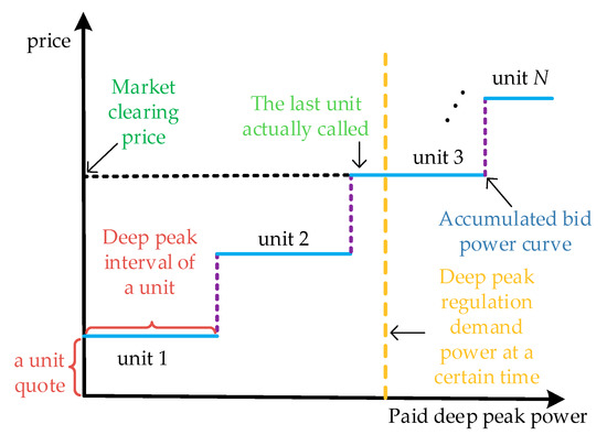
Figure 1.
Unification of the clearing price mechanism.
The stepped curve in Figure 1 represents the market cumulative bid power curve. At some time period, the deep peak regulation demand power is expressed by a straight line perpendicular to the abscissa axis. The market clearing price is the price corresponding to the intersection of the two curves. Solving the market clearing model with the goal of the market organizer purchasing minimum deep peak regulation auxiliary service. This process can be represented by the following optimization model:
where and are the market clearing price and bidding generation capacity of the strategic subject i in time t. is the maximum technical output of the strategic subject i. is the first-stage electrical power output of the strategy subject i in time t when corresponding to the bid amount upper limit expected value is maximum. and are the maximum and minimum electrical power ramping capability of the strategy subject i. is the market deep peak regulation demand power in time t. It can be predicted from historical data, and its uncertainty is not considered here to reduce the difficulty of solving.
This optimization model can be solved by the queuing method. The basic idea is to arrange the bidder’s quotations from low to high, and clear them out until the deep peak regulation demand is met. However, the simple queuing method is difficult to deal with the unit climbing rate constraint, so this paper uses the dynamic queuing method to solve. According to the above model, different quotation coefficients ai,s and bi,s were substituted into the value of ai and bi to calculation, the bidding generation capacity and market clearing price of the strategic subject i in time t can be obtained under different quotation scenarios s. Then compare the expected sales power profit of the bidding generation capacity of the strategic subject i with the expected deep peak regulation auxiliary service profit, to determine the time period Z(t,s) in which participating deep peak regulation auxiliary service market can obtain higher profits:
where s is the quotation scenarios. Z(t,s) is a binary variable, when Z(t,s) = 1 means that participating deep peak regulation auxiliary service market can obtain higher profits, otherwise Z(t,s) = 0. is the electricity price in time t.
Enter the market clearing price and bidding generation capacity of the strategic subject i in scenario s and time t, binary variable Z(t,s) and the first-stage electrical power output of the strategy subject i in time t when corresponding to the bid amount upper limit expected value is maximum as constants into the second-stage scheduling model.
3.2. Second-Stage Scheduling Model
In the second-stage scheduling model, the CHP unit used the energy storage of heat network to improve the flexibility of unit and reduce the two-stage output deviation. In order to ensure that the thermoelectric balance constraint after bidding can still be satisfied, the deviation compensation fee is introduced. When the self-regulating capacity of the CHP unit is insufficient, the peaking resource needs to be purchased and the compensation is paid. The uncertainty of the parameters is considered through stochastic programming, and the risk is managed by CVaR indicators.
3.2.1. Objective Functions
As mentioned above, the aim of the proposed second-stage scheduling model is to maximize total profits of the CHP unit in consideration of risk management. Therefore, this paper first gives the maximum expectation profit ProfExp in all scenarios expressed as below:
where is the probability of occurrence of quotation scenario s. Profs is the total profits of the CHP unit which is earned in scenario s.its expression is as follows:
where and are the profit of sale electricity and sale heat in scenario s, respectively. is the profit component when participates in the deep peak regulation auxiliary service market in scenario s. is the operated cost of the CHP unit in scenario s, the expression is as shown in Equation (6). is the deep peak regulation cost of the CHP unit in scenario s. is the penalty cost for the deviation of the CHP unit in scenario s, its a piecewise function that can be represented as a linear constraint Equation (31) for ease to solve.
The expressions of the above various benefits and costs are as follows:
(1) Profit of sale electricity power
where is the electrical power output of the CHP unit i in time t and scenario s. When 1 − Z(t, s) = 1, it means that the CHP unit i only participates in the electricity market in time t and scenario s. At present, the electricity spot market of China’s Northeast Power Grid has not yet been established, and the settlement method of sales electricity power sprofits is still the product of the on-grid electricity power and the on-grid price of coal-fired units.
(2) Profit component when participates in the deep peak regulation auxiliary service market
where is the profit component when participates in the deep peak regulation auxiliary service market in scenario s. It consists of the deep peak regulation auxiliary service profit of the bidding generation capacity and the actual electrical power output minus the sales profit of the part of the electricity after the bid. After the market clears out, the CHP unit reduces the electrical power output according to the winning bidding generation capacity in the bidding period, so it is necessary to subtract the sales profit from the winning bidding generation capacity. The market clearing price and bidding generation capacity of the strategic subject i in scenario s and time t are solved by the first-stage scheduling model.
(3) Profit of sale heat power
where is the price of sale thermal power output in time t. is the thermal power output of the CHP unit i in time t and scenario s.
(4) The deep peak regulation cost of the CHP unit
where φi is the cost coefficients for the unit deep peak regulation power of the CHP unit i.
The objective function expression that maximizes CVaR is as follows [24,32,33]:
where ξs is a auxiliary positive variable. VaR is the value-at-risk. ξs and VaR are calculated by the CVaR constraint.
Finally, the CVaR and expected value models are comprehensively considered by introducing weighting coefficients. The final objective function expression is as follows:
where θ is the weighting coefficients, also known as risk aversion coefficient θ reflects the attitude of strategic subject to risk. When θ = 0 means that the strategic subject does not pay attention to the risk loss caused by the system uncertainty factor, and does not take measures to avoid the risk. When θ = 1 means that strategic subject tend to be conservative in scheduling, indicating that strategic subject pursue lower risk losses.
3.2.2. Problem Constraints
The constraints related to CVaR, constraints related to district heating network, constraints related to node, constraints related to heat exchanger stations, constraints related to CHP unit, Constraints related to system are as follows:
(1) Deviation penalty constraint
The deviation penalty cost is proportional to the deviation amount, and its expression is a piecewise function. For the convenience of solving, it can be represented by a linear constraint:
where ζi is the cost coefficient for purchasing peak regulation service for CHP unit i. is the first-stage electrical power output of the CHP unit i in time t when corresponding to the bid amount upper limit expected value is maximum.
(2) CVaR constraint
In order to calculate the CVaR, the following linear constraints are also required:
(3) Constraints related to district heating network
This paper considers a District Heating Network consisting of supply and return pipelines. Figure 2 is a schematic diagram of DHN and nodes. The DHN’s control strategy generally regulates mass flow rates to meet thermal demand while maintaining supply and return temperatures within certain desired levels. In order to reduce heat losses, these limits can be adjusted according to the ambient temperature. In addition, in order to utilize the energy storage of the DHN as much as possible, this paper models temperature and mass flow rates as decision variables [34,35].
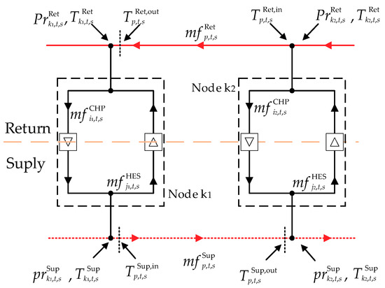
Figure 2.
Schematic diagram of DHN and nodes.
• Mass flow rates constraints in supply and return networks:
where and are the minimum and maximum mass flow rates of the supply pipelines p. and are the minimum and maximum mass flow rates of the return pipelines p. and are the minimum and maximum mass flow rates of the return pipelines p in time t and scenario s.
• Pressure loss caused by supply and return pipelines friction are defined as:
where k is the set of nodes in the district heating network. and are the pressure in node k in the supply and return network in time t and scenario s. νp is the pressure loss coefficient in pipeline p.
• The inlet temperature of the supply and return pipelines can be expressed as:
where and are the inlet temperatures in the supply and return pipeline p in time t and scenario s. and are the supply and return temperatures at node k in time t and scenario s.
• Temperature dynamic model and time delay in the supply and return pipeline:
The difficulty in modeling district heating network is to simulate the dynamic temperature in the pipeline and how the outlet temperature and delay time have been modeled. In this paper uses a first-order Taylor series expansion to approximate this problem [36]:
where are the outlet temperatures in the supply pipeline p in time t and scenario s. is the time delays in the supply pipeline p in time t and scenario s. μp is the thermal loss coefficient in pipeline p. c is the specific thermal capacity of water. ρwater is the density of water. Rp is the radius of pipeline p.
The discrete time delays can be expressed as [34,35,37]:
The longest time delay can be calculated using the physical characteristics of the pipeline p. Lp is the length of pipeline p. However, Equation (37) is non-linear, we need to introduce a binary auxiliary variable to linearize Equation (37), such that:
The term M is the a big-enough constant, so the discrete time delays after linearization can be expressed as:
Equation (36) is non-linear, we need to introduce variables Δ and the binary auxiliary variable to linearize Equation (36), such that:
As can be seen from Equations (40)–(43), = 1 and Δ≠ 0 if and only if = φ. In this example, . Therefore the linearized formula (36) can be expressed as:
In the same way, we can get the temperature dynamic model and time delay in the return pipeline, but in order to reduce the space, we do not list the detailed steps.
(4) Constraints related to nodez
The water flow is incompressible, so the net mass flow rate at each node of the heat network is equal to zero.
• Net mass flow rate at each node, can be expressed as:
where and are the set of pipelines with node k as ending and starting. is the set of the CHP unit connected to node k. and are the mass flow rates of the CHP unit i and heat exchanger stations j in time t and scenario s.
• Supply and return pressures at each node, can be expressed as:
where and are the minimum and maximum pressure at node k in the supply network. and are the minimum and maximum pressure at node k in the return network.
• The supply and return temperatures at the node k are equal to the mix of pipeline outlet temperatures converging to that node, can be expressed as:
where and are the supply and return temperatures in node k.
• The bounds of supply and return temperatures at the node k, can be expressed as:
where and are the minimum and maximum supply temperatures at node k. and are the minimum and maximum return temperatures at node k.
• For nodes where only one pipe arrives or leaves, Equation (47) can be replaced with the following linear constraint:
(5) Constraints related to heat exchanger stations
• Relationship between heat exchange station and heat load can be expressed as:
where is the thermal power generation load forecasting of the heat exchange station j in time t.
• Mass flow rates constraints of the heat exchange station can be expressed as:
where and are the minimum and maximum mass flow rates of the heat exchange station j.
The pressure differences between supply and return networks at heat exchange station must be greater than the threshold to ensure the mass flows rates:
where is the minimum pressure of the heat exchange station j.
(6) Constraints related to CHP unit
• Relationship between heat exchange station and heat load can be expressed as:
• Mass flow rates constraints of the CHP unit can be expressed as:
where and are the minimum and maximum mass flow rates of the CHP unit i.
• The power consumption of the water pump of the CHP unit i is positively related to the pressure differences between the supply and the return network:
where is the electricity power consumption of water pump of the CHP unit i in time t and scenario s. is the conversion efficiency of water pump of the CHP unit i.
The point feasible operating region constraints and climb ramp related constraints of CHP unit are as shown in Equations (9)–(11).
(7) Electricity power balance
where Lt,nmax is the electricity power generation load forecasting in time t when corresponding to the bid amount upper limit expected value is maximum.
3.2.3. Constraint Linearization
Due to the existence of the nonlinear term (6), (33),(46),(49),(52) and (54) the above model is a Mixed Integer Nonlinear Programming (MINLP) model, which greatly increases the difficulty and solution time of the model, so we must linearize these items and turn the problem into a Mixed Integer Linear Programming problem.
The linearization method of the fuel cost objective function Equation (6) of CHP unit is explained in [38]. The linearization method of the pressure loss constraints Equation (33) and constraints Equations (46), (49), (52) and (54) of CHPs unit are discussed in [35]. After linearizing the objective function and constraints, the CPLEX solver under GAMS software is used.
As shown in Figure 3, From the first-stage scheduling model, the time period Y(t) in which the market needs deep peak regulation auxiliary service is obtained, and the first-stage electrical power output when corresponding to the bid amount upper limit expected value is maximum. When Y(t) = 1, the strategy subject uses the particle swarm optimization (PSO) algorithm to determine its own optimal bidding coefficient. The strategy subject uses LHS to generate the competitor’s possible quotation scenario set s according to the competitor’s historical quotation data, and uses the dynamic queuing method to simulate the market clearing process, and obtains the clearing amount and market clearing price under the quotation scenario set s, and determines the time period Z(t,s) in which participating deep peak regulation auxiliary service market can obtain higher profits, These parameters are entered as constants into the scheduling model of the second-stage. After considering the expected profit and CVaR comprehensively, select the best particle, determine the final quotation coefficient a,b and report it.
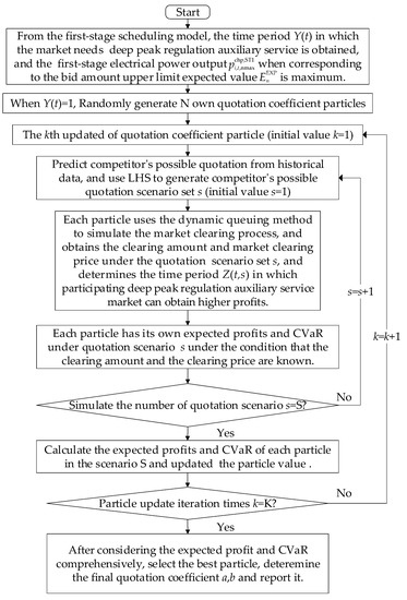
Figure 3.
Flow diagram of algorithm.
4. Simulation Cases and Results Analysis
4.1. Simulation System Basic Parameters
4.1.1. Power System Information
The structure of the simulation system shown in Figure 4 consists of two CHP plants and a condensing plant. The strategic subject of this paper is CHP plant A, which consists of two CHP units, one of which has a capacity of 330 MW and the other has a capacity of 300 MW. Assume that the competitor consists of CHP plant B and condensing power plant C. Each power plant contains two units. The unit parameters are shown in Table 2. The power generation cost function and operation constraints of the condensing unit extracted from [29]. The price of sale thermal power output is 14 $/(MW⋅h). The cost coefficients for the unit deep peak regulation power of the CHP unit i is 21 $/(MW⋅h). The cost coefficient for purchasing peak regulation service for CHP unit i is 11 $/(MW⋅h). Select price data and electrical load data for the Nord Pool market [39]. The thermal load demand curve of the strategic subject CHP A is shown in Figure 5. The electricity price is 61 $/(MW⋅h).
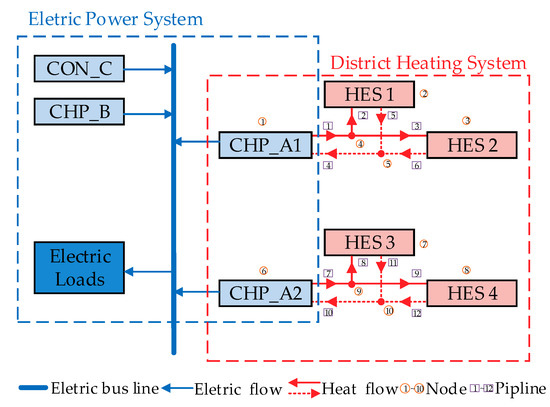
Figure 4.
Structure of the simulation system.
Table 2.
Parameter of Unit.
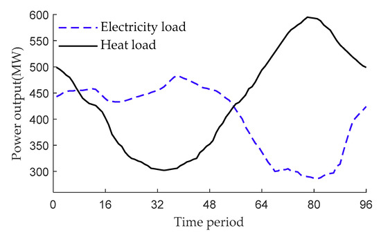
Figure 5.
Curves of heat load and electricity load.
This paper considers the bidding strategy of generators in the case of information symmetry, that is, each strategic subject has a mutual understanding of the possible quotation information of other strategic subject. For CHP unit A, this paper assumes μa = 60.34, μb = 0.232; for CHP unit B, μa = 60.54, μb = 0.248; for pure conglomerate power plant C, μa = 60.16, μb = 0.276.
4.1.2. Thermal System Information
The technical characteristics of the networks are derived from [35], and listed in Table 3 and Table 4.
Table 3.
Parameter of DHN.
Table 4.
Parameter of DHN node.
This paper considers that the specific thermal capacity of water c is 1.17 Whkg−2K−1 and the density of water is 1000 kgm−3. This article starts at 07:00 AM and divides 24 hours a day into 96 time intervals, each intervals is 15 minutes.
4.2. Case Study of CHPD and CED
4.2.1. Scheduling Model of the CED
The proposed combined heat and power dispatch considering energy storage of a district heating network (CHPD) model is compared to the conventional economic dispatch (CED) model to analyze the impact of DHN energy storage on the power system and to study its potential benefits. In the CED model, since the energy storage of the DHN is not considered, some modifications to the model of this paper are needed.
Specifically, constraints related to district heating network (32)–(43), constraints related to node (44)–(48), constraints related to heat exchanger stations (49)–(51), constraints related to CHP unit (52)–(54) is replaced by the following heat balance constraint:
Because the water pump was not modeled, the electricity power balance formula (55) was replaced with:
The other system constraints remain the same, the structure of the simulation system the same as Figure 4. Using the same linearization method, the nonlinear term is linearized into a Mixed Integer Linear Programming model.
4.2.2. Case Study
This section will explore the feasibility of the CHPD model using energy storage of DHN to decoupling electricity and heat dispatch. As shown in Figure 6a, in the CED model, the thermal power output of the CHP unit is strictly equal to the heat load demand value during each scheduling period.
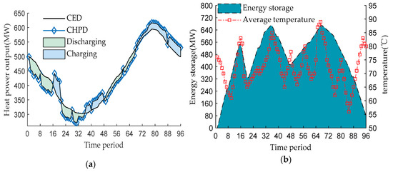
Figure 6.
Storage capacity of the DHN: (a) heat production and consumption. (b) average temperatures and total energy stored in pipelines.
In the CHPD model, the thermal power output of the CHP unit is no longer strictly equal to the heat load demand value at each scheduling period, but needs to meet the relevant physical constraints of the DHN. As shown in Figure 6a, the thermal power output of the CHP unit is not limited by the thermal load demand value for each dispatch period. But this does not contradict the law of conservation of energy in DHN. In fact, the water flow in the DHN is heated by the thermal power generated by the CHP unit, and the hot water flow is the carrier of the heat load. The injection of heat from the CHP unit or the withdrawal of heat results in the difference in energy storage in the DHN. The shaded portion in Figure 6a shows the energy change of DHN.
As shown in Figure 6a, DHN is used as an energy storage device. As indicated by the shaded portion, during charging periods, the CHP unit injects more energy into the pipeline than is required by the heat load. During the discharging periods, the energy consumed by the heat system exceeds the energy produced by the CHP unit, the vacancy is supplemented by energy storage in the DHN. The utilization of DHN energy storage is achieved by controlling the inlet temperature and mass flow rate of the pipeline. Most of the charging period is in the period of low demand heat load, and the discharge period is mostly in the period of high demand heat load.
The cumulative energy change of DHN and the average water temperature in the pipeline are shown in Figure 6b, it also can be seen that the average water temperature of the pipeline varies with the energy storage. Therefore, due to the heat capacity of the water flow, DHN can be used as a energy storage device, which will cushion the heat injection and withdrawals. It can decouple the power generation and heat demand of CHP units without affecting the quality of heating service, and improve the flexibility of CHP unit operation.
4.3. Analysis of Bidding Strategy Results
4.3.1. Cases Settings
In order to evaluate the ability of the proposed two-stage stochastic programming method to solve the optimal bidding problem between the electricity market and the deep peak regulation auxiliary service market, consider the following twelve cases (each three consecutive cases have their risk aversion coefficient θ value are set to 0, 0.5 and 1, respectively):
- E1 to E3: The strategy subject uses the CED model to only participate in the bidding of the electricity market.
- E4 to E6: The strategy subject uses the CED model to participate in the bidding of the electricity market and the deep peak regulation auxiliary service market.
- E7 to E9: The strategy subject uses the CHPD model to only participate in the bidding of the electricity market.
- E10 to E12: The strategy subject uses the CHPD model to participate in the bidding of the electricity market and the deep peak regulation auxiliary service market.
Among them, the model of E1 to E3 is based on the CED model of this paper, but removing the profit function and cost function and related constraints of deep peak auxiliary service. The model of E4 to E6 is based on the CED model of this paper. The model of E7 to E9 is based on the CHPD model of this paper, but removing the profit function and cost function and related constraints of deep peak auxiliary service. The model of E10 to E12 is the model proposed in this paper.
4.3.2. Results Analysis
The results of these cases are listed in Table 5. Comparing the results of E1 and E7, the use of energy storage of the district heating network led to an increase in expected profit of $8234 (4.6%) and a reduction in deviation penalty cost of $734. Although the CVaR weighting factor (θ) in the objective function is equal to zero in E7, it has been observed that the use of energy storage of the district heating network results in an increase in CVaR of $3433. This is because the energy storage function of the district heating network can reduce the occurrence of deviations and reduce the deviation penalty cost, to prevent violations of the proposed bid in the event of a deviation. The same can be seen by comparing the results of E4 and E10.
Table 5.
Optimization results by proposed two-stage SP method to solve the optimal bidding problem between the electricity market and the deep peak regulation auxiliary service market.
By comparing the results of E7 and E10, participation in both the electricity market and the deep peak regulation auxiliary service market increased the expected profit by $17,906 (9.5%) compared to only participation in the electricity market. This is because the market clearing price of the deep peak regulation auxiliary service market is mostly higher than the electricity price of the electricity market. In addition, the deviation penalty cost of only participating in the electricity market is $414 less than than participation in both the electricity market and the deep peak regulation auxiliary service market. The reason is that CHP’s ability to adjust the deviation is weakened when it provides deep peak auxiliary service. The deviation is mainly adjusted by the energy storage of district heating network, but the deviation penalty cost is reduced less than the deep peak auxiliary service profit, so the total profit of E10 is still higher. The same can be seen by comparing the results of E1 and E4.
By comparing the results of E10 to E12, as the risk aversion coefficient θ increases (i.e., the weight of the CVAR in the objective function increases and the weight of the expected profit in the objective function reduces), CVaR increases and the expected profit decreases. When θ is increased from 0 to 0.5 (i.e., compared to E11 and E12), the expected profit is reduced by $2,348, but CVaR is increased by $13,469. In the case of a slight reduction of the expected profit, the risk of profit is greatly increased. When risk aversion coefficient θ = 1(E12), expected profit was reduced by $64,875 compared to θ = 0(E10), but CVaR was only increased by $15,288. Therefore, in the three cases of E10 to E12, the value of risk aversion coefficient θ should be taken as 0.5 (E11) when the trade-off between expected profit and risk of profit is made. The same can be seen by comparing the results of E4 to E6. By comparing all the cases, we can find that CVaR increases significantly with the increase of θ. In addition, it is not difficult to find through the above comparison that after taking the risk factor into consideration, the expected profit obtained is reduced. But this does not mean that the actual profit will be reduced after considering the risk factors. It is not difficult to infer that the expected profit and the actual profit are not completely proportional. The mathematical relationship between them is complex. The higher the estimated expected profit, the CHP does not necessarily get more real profits. In the expectation value model, although the uncertainty variable is also considered, it is difficult to reflect the risk influence caused by the decision maker’s risk attitude and the extreme scene tail risk. When the risk factors are considered in the scheduling model, the influence of the uncertain variables on the profit can be better dealt with, and the loss caused by the low prediction accuracy of the uncertain variables can be reduced. Decision makers can determine the impact of uncertain operational risk on scheduling decisions based on their aversion to risk. This is closer to the actual situation. Therefore, it is necessary to consider the risk in the optimal bidding strategy. According to the algorithm flow of Figure 3, the time period which participates in deep peak regulation auxiliary services market for higher profit, deep peak regulation auxiliary market clearing price, the amount and quotation coefficient of deep peak regulation auxiliary services bids of each generator can be obtained.
This section only lists the quotation coefficients of the CHP A unit, which is the strategy subject of this paper. The quotation coefficients of other power producers are no longer listed. The quotation coefficients for E10 to E12 are shown in Table 6, Table 7 and Table 8, respectively
Table 6.
Bidding coefficient of CHP A for θ = 0(E10).
Table 7.
Bidding coefficient of CHP A for θ = 0.5(E11).
Table 8.
Bidding coefficient of CHP A for θ = 1(E12).
The bidding power and bidding curves for E10 to E12 are shown in Figure 7. As can be seen from Figure 7a,b, as θ increases (i.e., the strategic subject tends to be more risk averse), the optimal bid and the quotation will decrease. This is because the strategic subject tends to lower the optimal bid and the quotation to avoid being unable to win the bid in the deep peak regulation auxiliary service market.
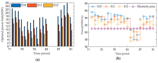
Figure 7.
Optimal power bids and bidding curves for cases E10 to E12: (a) optimal power bids; (b) bidding curves.
The market organizer summarizes the quotation information of all the power producers, and after clearing out according to the market clearing rules, the market clearing price and the winning power bid of each power producer can be obtained. This section only lists the market clearing price and the winning power bid of the CHP A unit, which is the strategy subject of this paper, as shown in Figure 8. The market clearing price and the winning power bid of other power producers are no longer listed. It can be seen from Table 6, Table 7 and Table 8 and Figure 8 that the bidding time period of CHP A is mainly concentrated in time period 72 to time period 91 (this article starts at 07:00 AM, and the time corresponding to this period is 01:00 AM–06:00 AM). The reason why the bidding time period is concentrated at 01:00 AM–06:00 AM is that, during this time period, a large number of CHP units operating on the principle of “power determined by heat”, resulting in system lack of the peak-load regulating capability, so additional peak-load regulating resources are urgently needed for compensation. As can be seen from Figure 8, at time periods 84, 85 and 86, CHP A unit did not participate in the bidding of the deep peak regulation auxiliary service market. This is because the market clearing price predicted during these time periods is less than the electricity price, during these periods, the profits from the participation of CHP A unit in the electricity market will be higher.
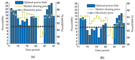
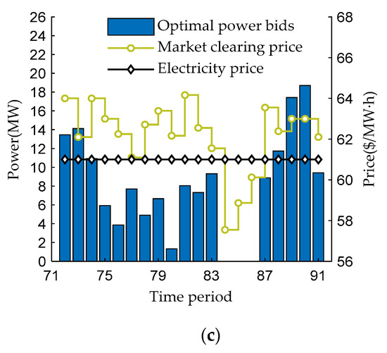
Figure 8.
Bidding power and bidding curve of CHP A unit: (a) θ = 0; (b) θ = 0.5; (c) θ = 1.
5. Conclusions
Aiming at the operation rules of the Northeast power peak auxiliary service market, this paper proposes a CHP unit bidding strategy based on two-stage stochastic programming risk-aversion model. The simulation results indicate that the energy storage capacity of the DHN can decouple the power generation and heat demand of CHP units without affecting the quality of heating service, and provide more operation flexibility. Compared to only participation in the electricity market, participation in both the electricity market and the deep peak regulation auxiliary service market increased the expected profit, and the use of energy storage of the district heating network can further increase the expected profits. Not all time periods that can participate in the deep peak regulation auxiliary service market are need to bidding, and it is necessary to compare the electricity price and the predicted deep peak regulation auxiliary service market clearing price to determine the time period for final bidding in the deep peak regulation auxiliary service market. It can be seen that the strategic subject tends to lower the optimal bid and the quotation to avoid being unable to win the bid in the deep peak regulation auxiliary service market when considering risks. It can also be seen in the objective function that if the expected profit and CVaR select the appropriate weighting factor, a suitable compromise between the expected profit and the CVaR optimal value can be obtained.
After the establishment of China’s Northeast Power Spot Market, the consideration of uncertainty of electricity prices in the optimal bidding problem are left for future work. In addition, how to further improve the operational flexibility of the CHP unit and enable it to participate in the second-level deep peak regulation auxiliary service market is a problem worth studying. The model in this paper uses a number of linearization steps to simplify the model, however, these linearization steps are extremely case-dependent and not necessarily suitable for other models. In addition, the method mentioned in the model of this paper has no practical application for the time being. Applying the method proposed in this paper to the actual system will be the work of the next stage. The problem that the practical application needs to solve is far more complicated than the model proposed in this paper. Especially for large and long pipelines, the temperature inside the pipeline is affected by the external temperature. How to deal with this problem deserves further study.
Author Contributions
L.T. and Y.X. conceived and designed the research framework. Y.X. and B.H. establish a scheduling model. X.L., and T.D. have written code for the scheduling model. H.L. and F.L. participated in the analysis of the results. L.T. supervised the writing of the thesis.
Funding
This research was funded by the National Key R&D Program of China under grant number 2017YFB0902100.
Conflicts of Interest
The authors declare no conflict of interest.
Abbreviations
The following abbreviations are used in this manuscript:
| CHP | Combined heat and power |
| CON | Condensing unit |
| DHN | District heating network |
| MCS | Monte Carlo simulation |
| LHS | Latin hypercube sampling |
| CVaR | Conditional value-at-risk |
| MCP | Market clearing price |
| CED | Conventional economic dispatch |
| CHPD | Combined heat and power dispatch consider energy storage of district heating network |
| SP | Stochastic programming |
| MILP | Mixed integer linear programming problem |
| MINLP | Mixed integer nonlinear programming |
| PSO | Particle swarm optimization |
References
- Liu, Y.Q.; Zhang, H.P.; Li, Q. Design and practice of peak regulation ancillary service market for northeast china power grid. Autom. Electr. Power Syst. 2017, 41, 148–154. [Google Scholar]
- Lin, L.; Tian, X.Y. Analysis of deep peak regulation and its benefit of thermal units in power system with large scale wind power integrated. Power Syst. Technol. 2017, 41, 2255–2263. [Google Scholar]
- Liu, P. Research on coal fired generator participating in peak valley dispatching ancillary service strategy. Northeast Electr. Power Technol. 2018, 39, 34–37. [Google Scholar]
- Li, P.; Zhao, S.Y.; Jin, S.J. Promotion method of peak regulation capacity by power and heat decoupling based on heat storage of district heating network and buildings. Autom. Electr. Power Syst. 2018, 42, 20–28. [Google Scholar]
- Peng, F.X.; Li, X.J.; Shun, H. Dispatch strategy for wind power accommodation considering coordination of power generation group stakeholders. Autom. Electr. Power Syst. 2018, 42, 98–108. [Google Scholar]
- Levihn, F. CHP and heat pumps to balance renewable power production: Lessons from the district heating network in Stockholm. Energy 2017, 137, 670–678. [Google Scholar] [CrossRef]
- Averfalk, H.; Ingvarsson, P.; Persson, U.; Gong, M.; Werner, S. Large heat pumps in Swedish district heating systems. Renew. Sust. Energy Rev. 2017, 79, 1275–1284. [Google Scholar] [CrossRef]
- Yu, J.; Guo, L.; Ma, M.; Kamel, S.; Li, W.; Song, X. Risk assessment of integrated electrical, natural gas and district heating systems considering solar thermal CHP plants and electric boilers. Int. J. Electr. Power Syst. 2018, 103, 277–287. [Google Scholar] [CrossRef]
- Nielsen, M.G.; Morales, J.M.; Zugno, M.; Pedersen, T.E.; Madsen, H. Economic valuation of heat pumps and electric boilers in the Danish energy system. Appl. Energy 2016, 167, 189–200. [Google Scholar] [CrossRef]
- Katulić, S.; Čehil, M.; Bogdan, Ž. A novel method for finding the optimal heat storage tank capacity for a cogeneration power plant. Appl. Therm. Eng. 2014, 65, 530–538. [Google Scholar] [CrossRef]
- Romanchenko, D.; Kensby, J.; Odenberger, M.; Johnsson, F. Thermal energy storage in district heating: Centralised storage vs. storage in thermal inertia of buildings. Energy Convers. Manag. 2018, 162, 26–38. [Google Scholar] [CrossRef]
- Franco, A.; Versace, M. Multi-objective optimization for the maximization of the operating share of cogeneration system in District Heating Network. Energy Convers. Manag. 2017, 139, 33–44. [Google Scholar] [CrossRef]
- Franco, A.; Bellina, F. Methods for optimized design and management of CHP systems for district heating networks (DHN). Energy Convers. Manag. 2018, 172, 21–31. [Google Scholar] [CrossRef]
- Vanhoudt, D.; Claessens, B.J.; Salenbien, R.; Desmedt, J. An active control strategy for district heating networks and the effect of different thermal energy storage configurations. Energy Build. 2018, 158, 1317–1327. [Google Scholar] [CrossRef]
- Borelli, D.; Devia, F.; Lo Cascio, E.; Schenone, C.; Spoladore, A. Combined Production and Conversion of Energy in an Urban Integrated System. Energies 2016, 9, 817. [Google Scholar] [CrossRef]
- Jing, Z.X.; Jiang, X.S.; Wu, Q.H.; Tang, W.H.; Hua, B. Modelling and optimal operation of a small-scale integrated energy based district heating and cooling system. Energy 2014, 73, 399–415. [Google Scholar] [CrossRef]
- Gazafroudi, A.S.; Soares, J.; Ghazvini, M.A.F.; Pinto, T.; Vale, Z.; Corchado, J.M. Stochastic interval-based optimal offering model for residential energy management systems by household owners. Int. J. Electr. Power 2019, 105, 201–219. [Google Scholar] [CrossRef]
- Renani, Y.K.; Ehsan, M.; Shahidehpour, M. Day-Ahead Self-Scheduling of a Transmission-Constrained GenCo With Variable Generation Units Using the Incomplete Market Information. IEEE Trans. Sustain. Energy 2017, 8, 1260–1268. [Google Scholar] [CrossRef]
- Su, W.; Wang, J.; Roh, J. Stochastic Energy Scheduling in Microgrids With Intermittent Renewable Energy Resources. IEEE Trans. Smart Grid 2014, 5, 1876–1883. [Google Scholar] [CrossRef]
- Panda, R.; Tiwari, P.K. Economic risk-based bidding strategy for profit maximisation of wind-integrated day-ahead and real-time double-auctioned competitive power markets. IET Gener. Transm. Distrib. 2019, 13, 209–218. [Google Scholar] [CrossRef]
- Shi, L.; Luo, Y.; Tu, G.Y. Bidding strategy of microgrid with consideration of uncertainty for participating in power market. Int. J. Electr. Power 2014, 59, 1–13. [Google Scholar] [CrossRef]
- Ding, H.; Pinson, P.; Hu, Z.; Song, Y. Optimal Offering and Operating Strategies for Wind-Storage Systems With Linear Decision Rules. IEEE Trans. Power Syst. 2016, 31, 4755–4764. [Google Scholar] [CrossRef]
- Aghaei, J.; Barani, M.; Shafie-khah, M.; de la Nieta, A.A.S.; Catalão, J.P.S. Risk-Constrained Offering Strategy for Aggregated Hybrid Power Plant Including Wind Power Producer and Demand Response Provider. IEEE Trans. Sustain. Energy 2016, 7, 513–525. [Google Scholar] [CrossRef]
- Akbari, E.; Hooshmand, R.-A.; Gholipour, M.; Parastegari, M. Stochastic programming-based optimal bidding of compressed air energy storage with wind and thermal generation units in energy and reserve markets. Energy 2019, 171, 535–546. [Google Scholar] [CrossRef]
- Barroso, L.A.; Conejo, A.J. Decision making under uncertainty in electricity markets. In Proceedings of the 2006 IEEE Power Engineering Society General Meeting, Montreal, QC, Canada, 18–22 June 2006. [Google Scholar]
- Rockafellar, R.T.; Uryasev, S. Conditional value-at-risk for general loss distributions. J. Bank. Financ. 2002, 26, 1443–1471. [Google Scholar] [CrossRef]
- Shi, J.Q.; Wang, Y.R.; Fu, R.B.; Zhang, J.H. Operating Strategy for Local-Area Energy Systems Integration Considering Uncertainty of Supply-Side and Demand-Side under Conditional Value-At-Risk Assessment. Sustainability 2017, 9, 1655. [Google Scholar] [CrossRef]
- Wei, W.; Yan, X.G.; Ni, Y.T.; Luo, F. Power System Flexibility Scheduling Model For Wind Power Integration Considering Heating System. In Proceedings of the 2017 IEEE Power & Energy Society General Meeting, Chicago, IL, USA, 16–20 July 2017. [Google Scholar]
- Li, P.; Wang, H.X.; Lv, Q.; Li, W.D. Combined Heat and Power Dispatch Considering Heat Storage of Both Buildings and Pipelines in District Heating System for Wind Power Integration. Energies 2017, 10, 893. [Google Scholar] [CrossRef]
- Gao, Y.; Zhou, X.; Ren, J.; Wang, X.; Li, D. Double Layer Dynamic Game Bidding Mechanism Based on Multi-Agent Technology for Virtual Power Plant and Internal Distributed Energy Resource. Energies 2018, 11, 3072. [Google Scholar] [CrossRef]
- Prabavathi, M.; Gnanadass, R. Energy bidding strategies for restructured electricity market. Int. J. Electr. Power 2015, 64, 956–966. [Google Scholar] [CrossRef]
- Hemmati, R.; Saboori, H.; Saboori, S. Stochastic risk-averse coordinated scheduling of grid integrated energy storage units in transmission constrained wind-thermal systems within a conditional value-at-risk framework. Energy 2016, 113, 762–775. [Google Scholar] [CrossRef]
- Vardanyan, Y.; Madsen, H. Optimal Coordinated Bidding of a Profit Maximizing, Risk-Averse EV Aggregator in Three-Settlement Markets Under Uncertainty. Energies 2019, 12, 1755. [Google Scholar] [CrossRef]
- Li, Z.G.; Wu, W.C.; Shahidehpour, M.; Wang, J.H.; Zhang, B.M. Combined Heat and Power Dispatch Considering Pipeline Energy Storage of District Heating Network. IEEE Trans. Sustain. Energy 2016, 7, 12–22. [Google Scholar] [CrossRef]
- Mitridati, L.; Taylor, J.A. Power Systems Flexibility from District Heating Networks. In Proceedings of the 2018 Power Systems Computation Conference (PSCC), Dublin, Ireland, 11–15 June 2018. [Google Scholar]
- Sandou, G.; Font, S.; Tebbani, S.; Hiret, A.; Mondon, C.; Tebbani, S.; Hiret, A.; Mondon, C. Predictive Control of a Complex District Heating Network. In Proceedings of the 44th IEEE Conference on Decision and Control, Seville, Spain, 15 December 2005. [Google Scholar]
- Li, Z.G.; Wu, W.C.; Wang, J.H.; Zhang, B.M.; Zheng, T.Y. Transmission-Constrained Unit Commitment Considering Combined Electricity and District Heating Networks. IEEE Trans. Sustain. Energy 2016, 7, 480–492. [Google Scholar] [CrossRef]
- Moradi, S.; Ghaffarpour, R.; Ranjbar, A.M.; Mozaffari, B. Optimal integrated sizing and planning of hubs with midsize/large CHP units considering reliability of supply. Energy Convers. Manag. 2017, 148, 974–992. [Google Scholar] [CrossRef]
- Nord Pool Website. Available online: https://www.nordpoolgroup.com/elspot-price-curves/ (accessed on 10 May 2019).


© 2019 by the authors. Licensee MDPI, Basel, Switzerland. This article is an open access article distributed under the terms and conditions of the Creative Commons Attribution (CC BY) license (http://creativecommons.org/licenses/by/4.0/).