RSSI-Power-Based Direction of Arrival Estimation of Partial Discharges in Substations

Abstract

The localization of partial discharges in air-insulated substations using ultra-high frequency technology is widely studied for power equipment early warning purposes. Ultra-high frequency partial discharge localization systems are usually based on the time-difference of electromagnetic wave signals. However, the large size of test equipment and the need for a high sampling rate and time synchronization accuracy limit their practical application. To address this challenge, this paper proposes a power-based partial discharge direction of arrival method using a received signal strength indicator from an ultra-high frequency wireless sensor array. Furthermore, the Gaussian mixture model is used for noise suppression, and the Gaussian process classifier is used for line of sight received signal strength indicator data identification. Laboratory tests are performed and the results show the average error of direction of arrival is less than 5°. The results verify the effectiveness of the proposed partial discharge localization system.

1. Introduction

Partial discharges (PDs) are one of the main factors of insulation deterioration and equipment break- down in air-insulated substations (AIS) [1,2]. Thus, monitoring and localization of partial discharges is an important topic in power systems. Much research has been done on the use of PD detection for condition monitoring and diagnosis of power equipment failure [3,4,5,6]. The authors in [2,7,8] used electromagnetic waves to locate PD sources and used the information for an early warning system in AIS. The localization methods are usually based on time of arrival (ToA) or time difference of arrival (TDoA) [9,10,11]. Some researchers have adopted array processing technology, i.e., multiple signal classification (MUSIC) [12] for better accuracy. However, these methods are mainly based on time-frequency analysis and therefore bear a high cost due to the requirement for nanosecond high accuracy time synchronization and high sampling rates of several gigahertz. Recently, some researchers have used received signal strength indicator (RSSI) methods to locate the PD sources and reduce the cost [13,14,15]. The standard RSS and RSSI localization techniques are usually divided into two stages, an offline stage to collect RSSI values in the detection area and an online stage to estimate the PD location by a scenario analysis method, so standard RSS and RSSI localization techniques usually have more workload and are less feasible for practical application due to the offline stage which is needed for building a fingerprints map [16].

This paper presents a simple method for PD direction of arrival (DoA) method by ultra-high frequency (UHF) RSSI measurements. Firstly, a circle array composed of UHF wireless sensors is designed and used for PD DoA. Then, the Gaussian mixture model (GMM) and Gaussian process classifier (GPC) are taken into consideration for reducing noise and line of sight (LOS) signal identification, respectively. Finally, the radiation characteristics of the designed UHF antenna is used for DoA through searching for the minimal RSSI value. To verify the proposed algorithm, a field test is carried out in a high voltage (HV) test laboratory. The main advantage of the proposed method is to achieve a similar accuracy comparing to the ToA or TDoA in a low hardware cost way.

The rest of the paper is organized as follows: Section 2 introduces the hardware of the sensor and the principle of the RSSI power-based DoA estimation. Section 3 describes the process of the DoA estimation in details. Section 4 presents the experimental results and Section 5 concludes the paper.

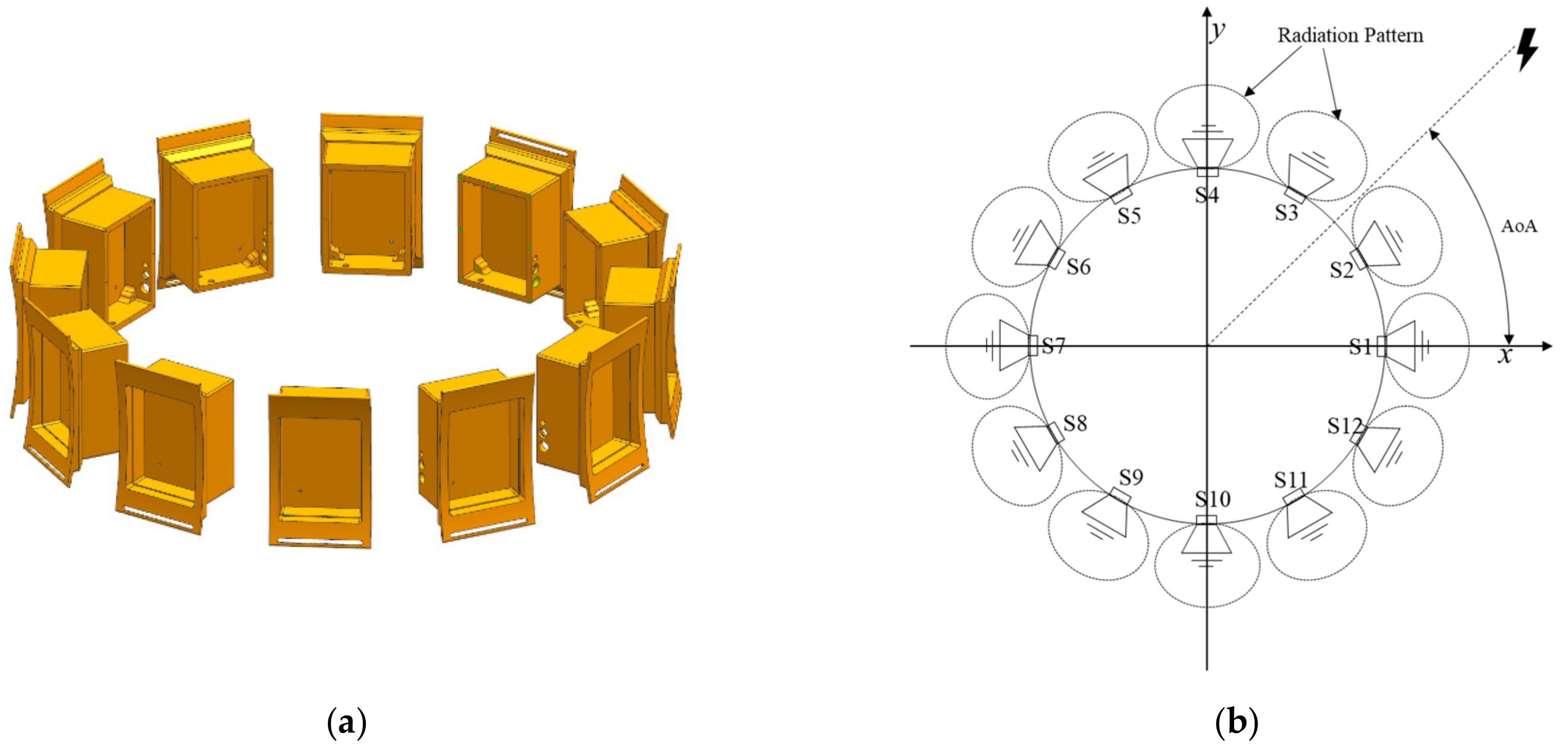
2. Fundamentals of DoA Estimation System

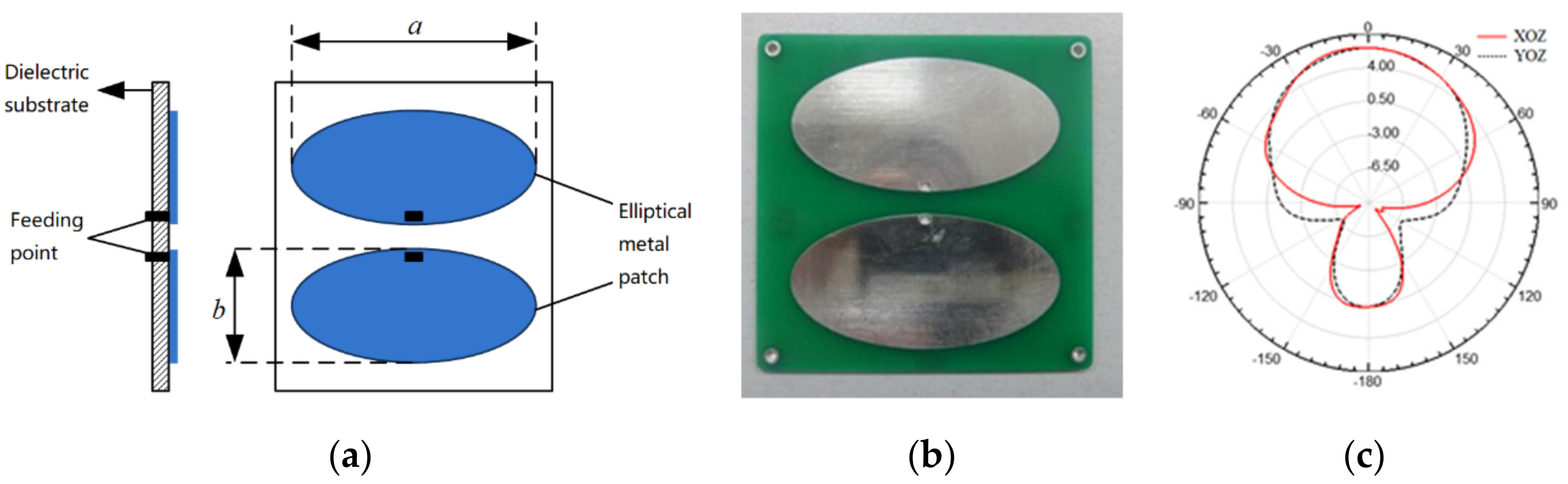
2.1. Wireless UHF Sensor

The UHF antenna we used is a printed circuit board (PCB) elliptical dipole antenna with double feed. A diagram and picture of the elliptical dipole antenna are shown in Figure 1a,b. The antenna’s 2-D radiation pattern at 1100 MHz is shown in Figure 1c. Figure 1c shows that the antenna has maximum sensitivity at 0°, and its minimum at 90° and −90°. Furthermore, the sensitivity at 180° is somewhat increased. Considering the electromagnetic shielding effect of the metal framework, the sensor has its maximum signal when the PD is in front of the sensor and the sensor has its minimal signal when the PD is behind the sensor.

For the designed wireless UHF sensors, the signal bandwidth is 300–1500 MHz and the A/D sampling rate is 2.7 MHz. Firstly, the UHF electromagnetic wave is received by the UHF antenna. Then, the envelope detection waveform is obtained after signal conditioning by a bandpass filter, amplifier and detector. Finally, the digital data are generated after A/D sampling and transmitted to computer through a Wi-Fi module controlled by MCU. The peak value of envelope detection waveform is the signal strength as we needed. The diagram and picture of the wireless UHF sensor are shown in Figure 2, respectively.

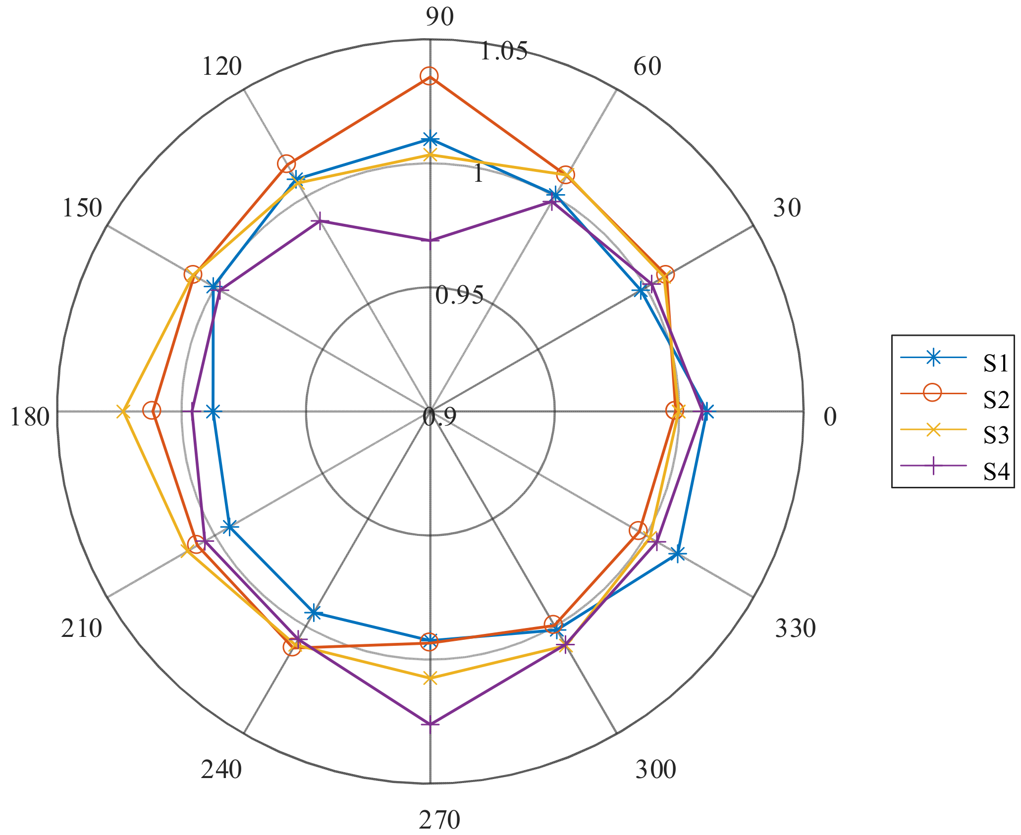
2.2. Preliminary Test of Radiation Pattern

The proposed DoA algorithm is based on the characteristic radiation pattern of the designed UHF sensor, thus, a preliminary test with four sensors was performed. The sensor array is comprised of four sensors and the four sensors are labeled as S1, S2, S3 and S4, respectively. The azimuth angle difference of every two adjacent sensors is 90°, and the angles of each sensor in the sensor array are assumed as 0°, 90°, 180° and 270° for convenience. When a PD event occurs, the DoA estimation result is regarded as angle difference between the DoA and the first sensor S1. In the preliminary test, the angle where the PD happens is from 0° to 360° and at an interval of 30°. The preliminary test result is shown in Figure 3.

The results in Figure 3 convey that the minimum value of each sensor is received when a PD event occurs behind the sensor in an ideal situation. Almost the maximum value is achieved in front of the sensor, however there is a little deviation from the expected angle. Besides the maximum and minimum values, the received value of each sensor fluctuates randomly at other angles. Therefore, this paper chooses to search for the minimal signal of the sensor array and then to find the direction of the arrival of PD. The angle of direction of the arrival is obtained by adding or subtracting 180° from the angle of the minimal signal.

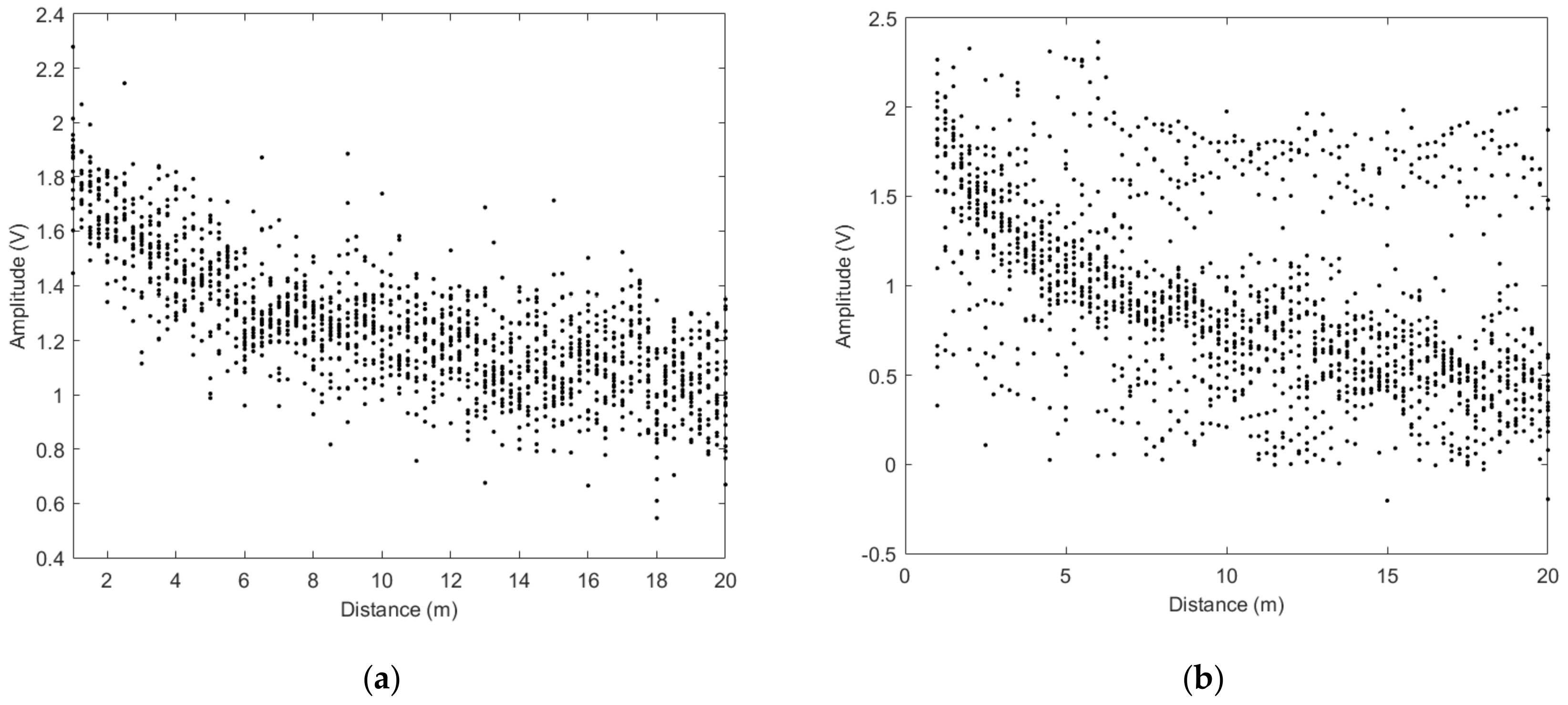
2.3. LOS and NLOS Consideration

Due to the complex environment of substations, i.e., the number of reflective surfaces due to installed power equipment, PD UHF signals will be severely impacted by shadowing and multipathing effects. This effect is referred to as the no-line of sight (NLOS) condition and has a high impact on the received RSSI data. Accordingly, the unobstructed scenario is called line of sight (LOS) conditions.

In order to investigate the influence of NLOS conditions on the received RSSI data, we also performed experiments in a laboratory environment that contains many pieces of power equipment to collect UHF RSSI data using wireless UHF sensors. Using the wireless UHF sensors, we measured and collected the RSSI values along 20 m in both unobstructed space and the laboratory environment. The experimental process is described simply as follows: the wireless UHF sensor is placed at a fixed point, then the distance between the simulated PD source and sensor is gradually changed in a straight line, and an air discharge pulse according to EN/IEC 61000-4-2 is generated by a PD simulator named ‘EM TEST DITO’ [17], and finally, the raw RSSI measurements at each position are collected. The parameters of the PD simulator are set as an inception voltage is 2 kV, a rise time is 0.7 ns and the spectrum is 0–1.5 GHz.

We collected total 1540 data under LOS conditions, reported in Figure 4a. Similarly, a total of 1540 data are collected under NLOS conditions and reported in Figure 4b. We can see that NLOS observations will make the signal amplitude more dispersed, and its attenuation trend is obviously different from LOS conditions. Therefore, NLOS condition can seriously affect the accuracy of the signal amplitude measurement, and thus affect the PD source DoA accuracy.

3. Methodology of RSSI-Power-Based PD DOA in Substations

3.1. Gaussian Mxiture Model for Noise Suppression

According to the signal attenuation model [18], the received signal strength indicator at the received wireless sensor can be calculated as:

$$P(d)=P(d_0)+10\gamma \lg (\frac{d}{d_0})+X_{\sigma }$$

(1)

where d₀ is the reference node and P(d₀) is corresponding RSSI, and γ is the attenuation coefficient which usually is known. X_σ follows a Gaussian distribution with mean value 0 and variance σ², so the RSSI of each sensor can be regarded as a Gaussian distribution. However, in a real situation, the received dataset is blended with noisy data. GMM is used to pick out the main Gaussian distribution and remove the noisy data [19].

GMM can be applied to divide the dataset or vectors into M Gaussian functions. The Gaussian mixture density is a weighted sum of M component densities:

$$f(x;\lambda )={\displaystyle \sum _{i=1}^M{p}_i{b}_i(x)}$$

(2)

where x is a D-dimensional vector, p_i is the mixture weight and satisfies the constrain that ${\displaystyle {\sum }_{i=1}^M{p}_i}=1$ The density function of b_i(x) is written as:

$$b_i(x)=\frac{1}{{(2\pi )}^{D/2}{\left|{\sum }_i\right|}^{1/2}}\exp \left\{-\frac{1}{2}{(x-{\mu }_i)}^T{\sum }_i{}^{-1}(x-{\mu }_i)\right\}$$

(3)

μ_i is the mean vector and Σ_i is the covariance matrix, so the Gaussian mixture density is parameterized by the mean vectors, covariance matrices and mixture weights. These parameters are collectively represented by the notation:

$$\lambda =\left\{{\mu }_i,{\sum }_i,p_i\right\} i=1,2,\dots ,M$$

(4)

In this paper, diagonal covariance matrices are used, and the most popular method to estimate the parameters of GMM is maximum likelihood (ML) estimation. The GMM likelihood can be written as:

$$P(x;\lambda )={\displaystyle \prod _{i=1}^{M}b(x_i,\lambda )}$$

(5)

The purpose of ML estimation is to find the target parameters that maximize the likelihood of GMM:

$${\widehat{\lambda }}_{\mathrm{ML}}=\arg \underset{\lambda }{\max } P(x;\lambda )$$

(6)

The target parameters can be obtained by the expectation maximization (EM) algorithm rather than by solving the nonlinear function. The EM algorithm begins with an initial parameter and estimating a new parameter which meets the condition that:

$$P(x;\widehat{\lambda })\ge P(x;\lambda )$$

(7)

Then the new parameter becomes the new initial parameter for the next iteration, and the iteration process is repeated until some convergence threshold is reached. After the above procedure, the main Gaussian distribution can be obtained for the next step.

3.2. Calibration and Normalization

In the selected dataset ψ‘:

$${\psi }^{\prime }=\left[\begin{array}{cccc}{s^{\prime }}_{1,1}& {s^{\prime }}_{1,2}& \cdots & {s^{\prime }}_{1,12}\\ {s^{\prime }}_{2,1}& {s^{\prime }}_{2,2}& \cdots & {s^{\prime }}_{2,12}\\ ⋮& ⋮& \ddots & ⋮\\ {s^{\prime }}_{m,1}& {s^{\prime }}_{m,2}& \cdots & {s^{\prime }}_{m,12}\end{array}\right]=\left[{S^{\prime }}_1,{S^{\prime }}_2,\cdots ,{S^{\prime }}_{12}\right]$$

(8)

Each column vector is represented by a sensor’s RSSI and each row vector is represented by all twelve sensors’ RSSI data once the PD happens. However, there are minor differences between the twelve sensors when the sensors are facing the same PD. Therefore, the calibration is done before the PD test by randomly selecting one sensor as a base, and in this paper the sensor S1 is regarded as base. In the same situation, the twelve sensors’ RSSI data for the same PD can be written as [F₁, F₂, …, F₁₂]. The calibration coefficient f_i for each sensor to S1 is written as:

$$f_i=\frac{F_i}{F_1} i=1,2,\cdots ,12$$

(9)

The calibration for the selected dataset is calculated by:

$$\psi =\left[\begin{array}{cccc}{s}_{1,1}& s_{1,2}& \cdots & s_{1,12}\\ s_{2,1}& s_{2,1}& \cdots & s_{2,12}\\ ⋮& ⋮& \ddots & ⋮\\ s_{m,1}& s_{m,2}& \cdots & s_{m,12}\end{array}\right]=\left[\frac{{S^{\prime }}_1}{f_1},\frac{{S^{\prime }}_2}{f_2},\cdots ,\frac{{S^{\prime }}_{12}}{f_{12}}\right]$$

(10)

After calibration, each data in the new matrix ψ can be updated by normalization in each row vector:

$$s_{i,j}=\frac{s_{i,j}}{{\displaystyle \sum _{j=1}^{12}{s}_{i,j}}/12} i=1,2,\cdots ,m$$

(11)

The calibration and normalization can reduce the DoA estimation error effectively. The error can be improved by approximately 15 percent.

3.3. LOS Identification by GPC

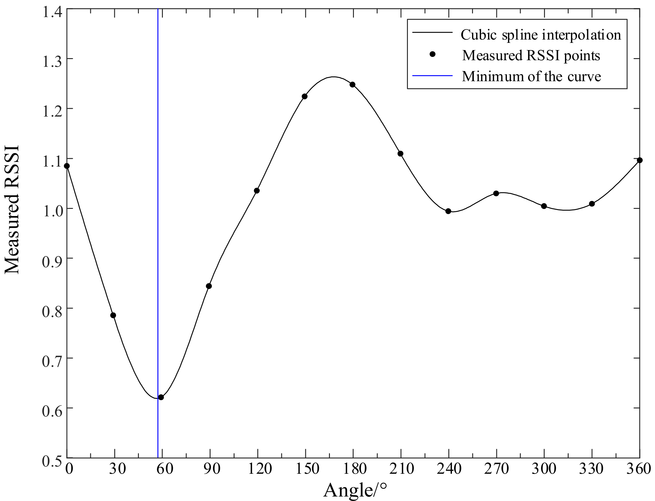
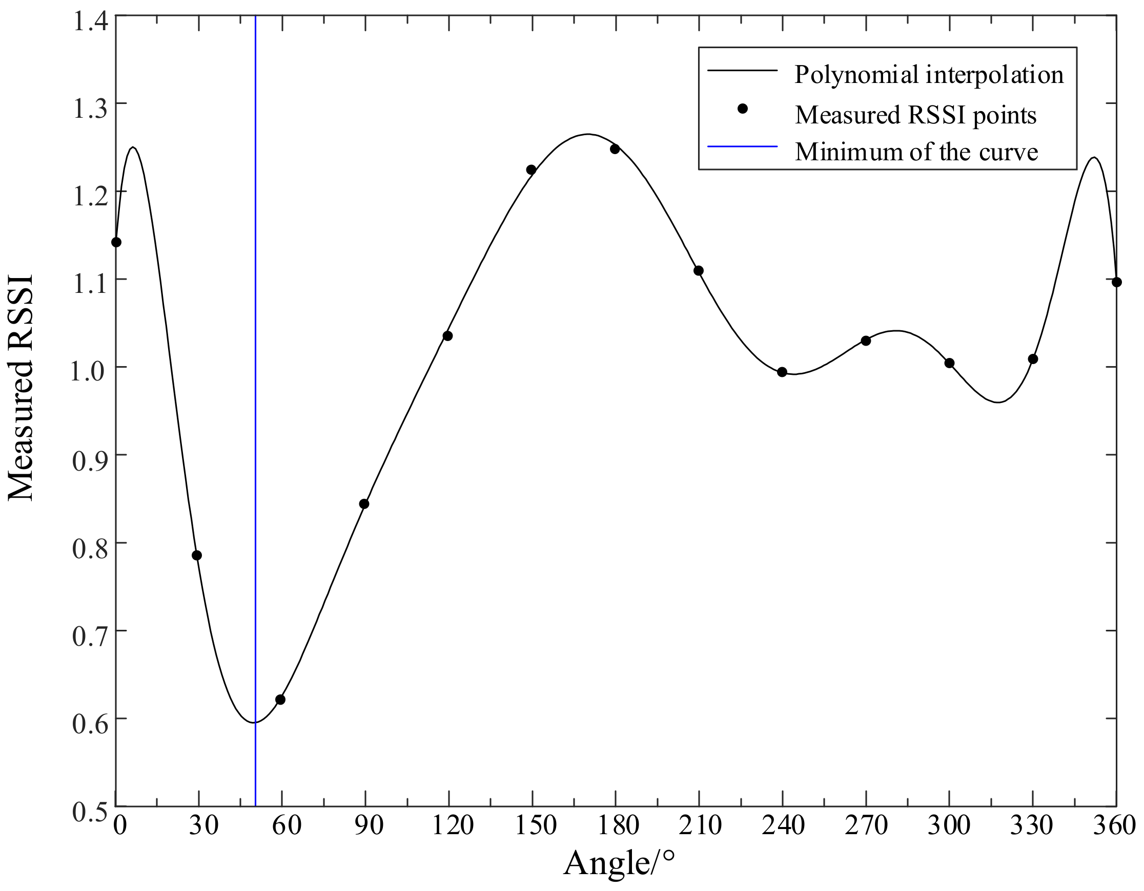
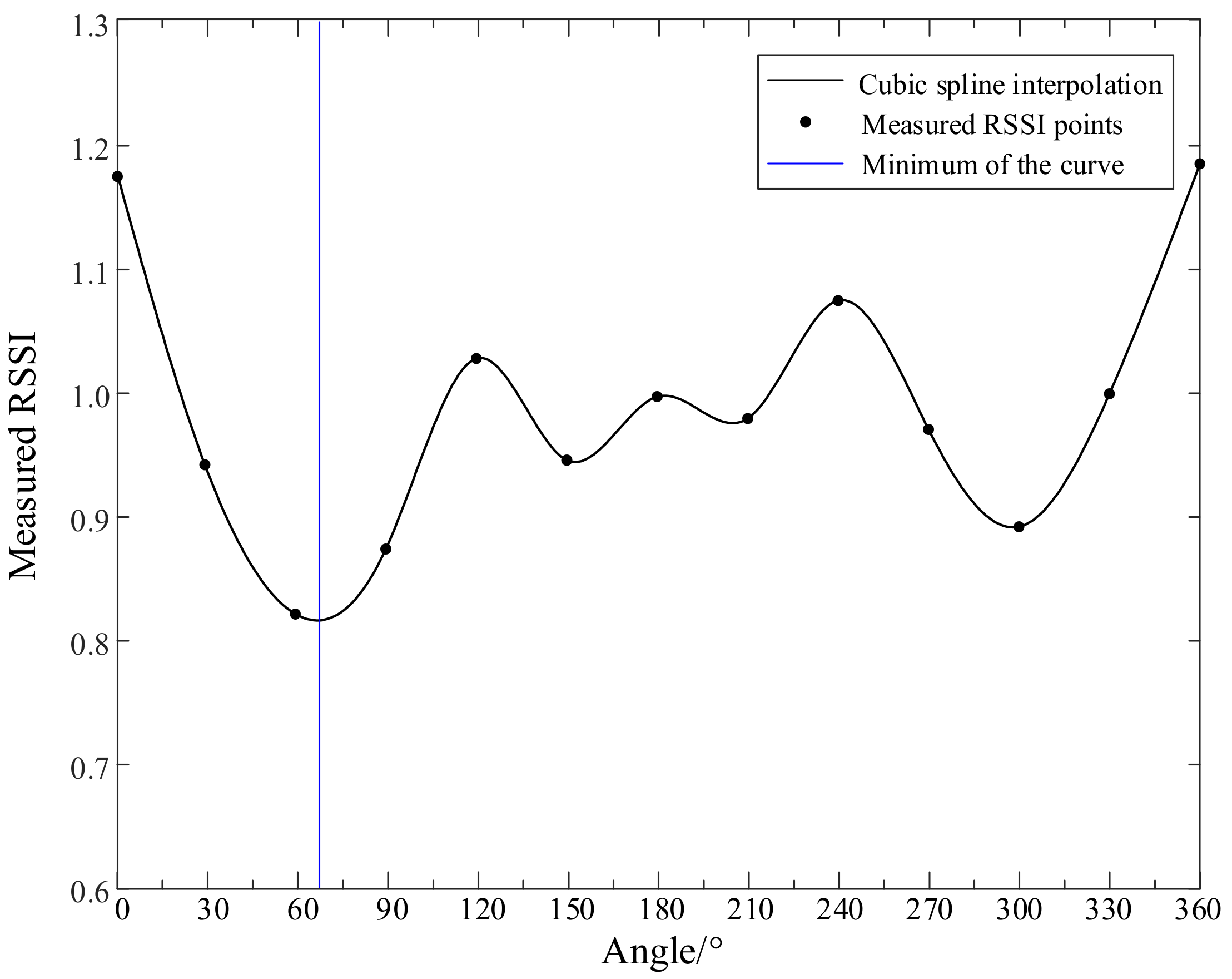
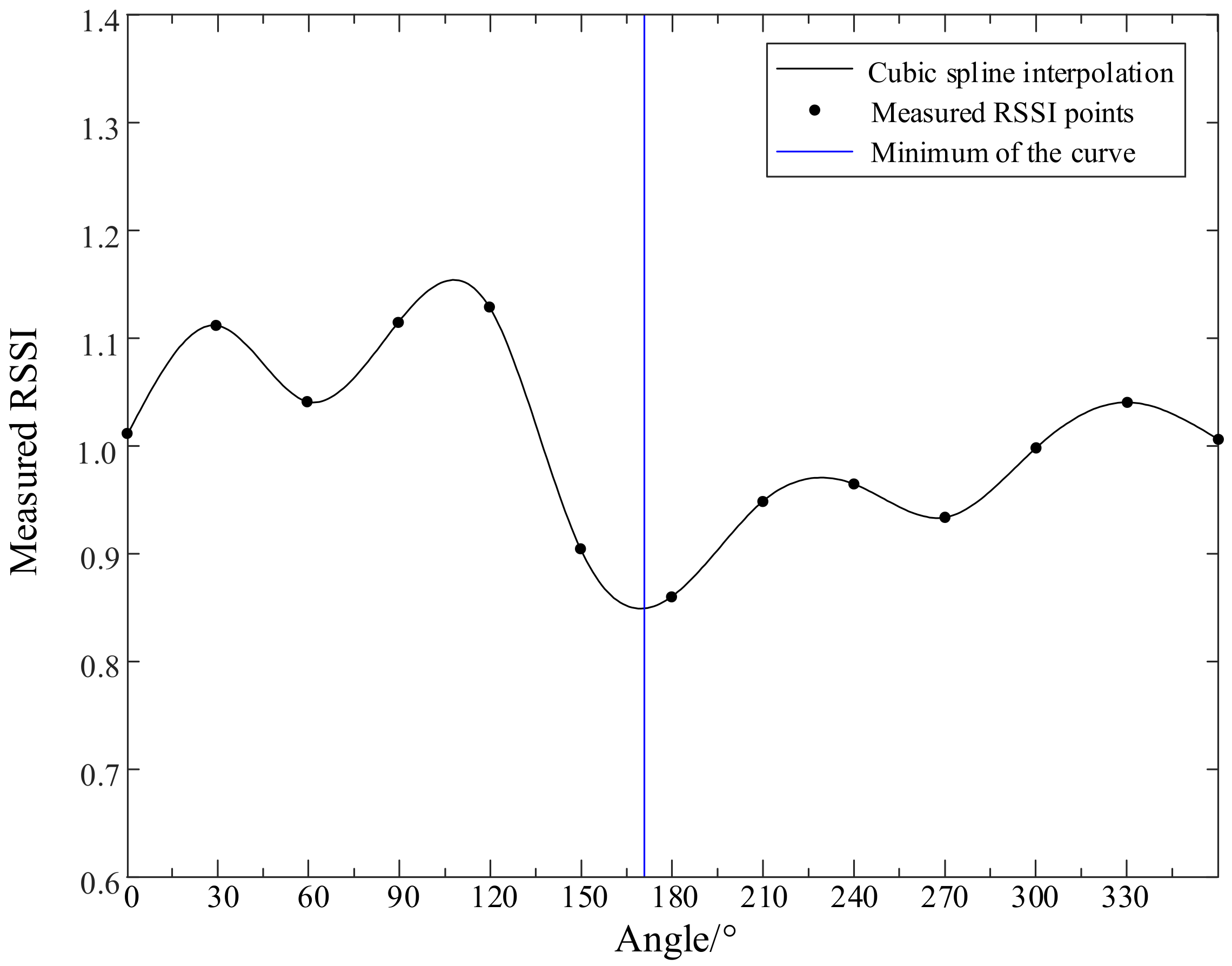
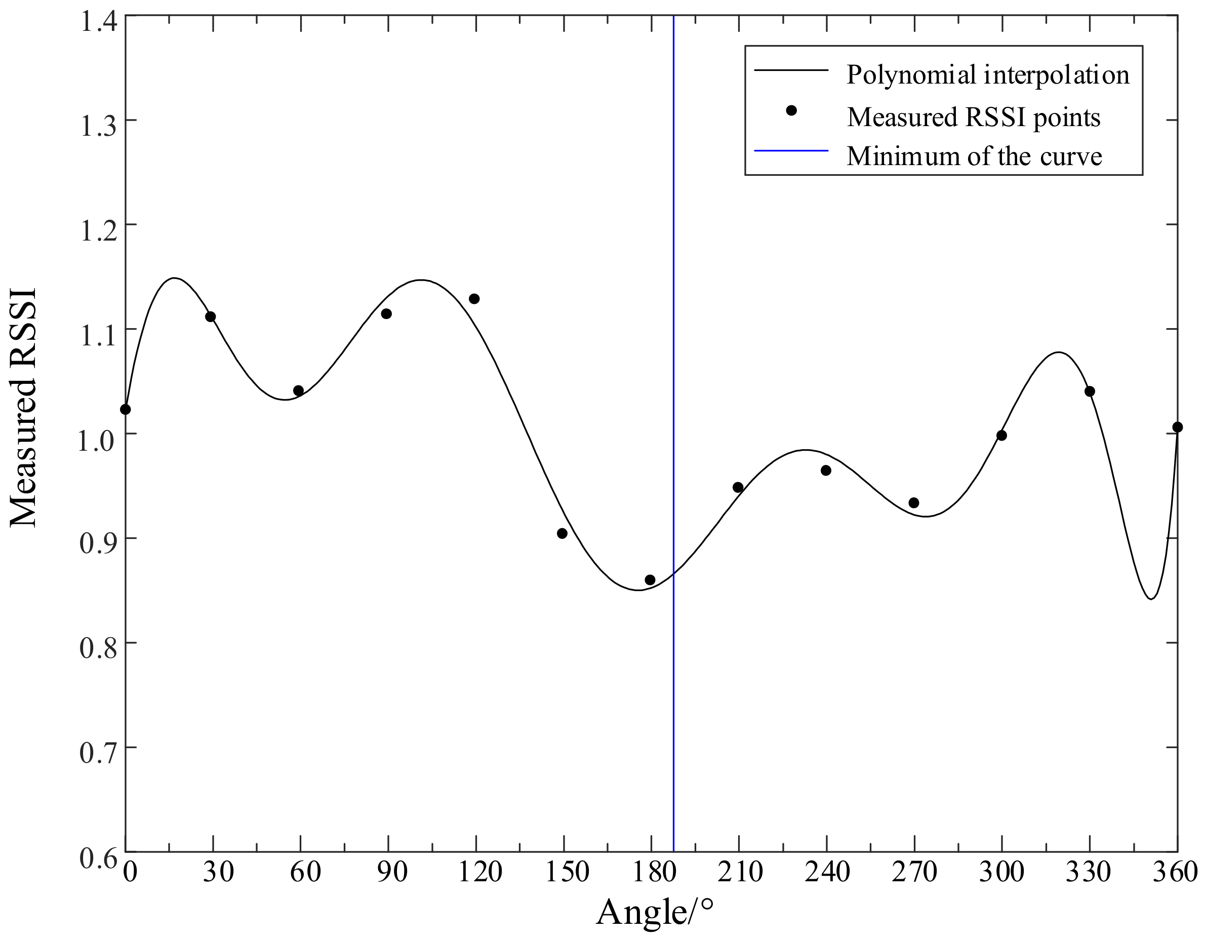
As addressed in Section 2.3, NLOS will affect the RSSI data significantly. Thus, a GPC is designed to determine the decision region of LOS/NLOS conditions. LOS/NLOS condition separation could be abstracted as a supervised classification problem of learning input output relationship from a training dataset. A machine learning technology named Gaussian process classification [20] provides us with a nonparametric Bayesian approach to learn the points dependencies of a dataset.

Supposing there are d sensors used for UHF monitoring and n samples obtained. Then, we define the training set $D\triangleq \left\{(x_i,y_i)|i=1,2,\dots n\right\}$ which contains a d-dimensional vector x and a d-dimensional class label vector y, $y=\{b_1,b_2,\dots b_d\}$, $b_j\in \left\{1,-1\right\}$.

Firstly, the latent predictive distribution of training set is computed by:

$$Y=f(X)+\epsilon$$

(12)

where $X=\left\{x_i,i=1,2,\dots n\right\}$ is a $d\times n$ matrix of aggregated input vectors x, and $Y=\left\{y_i,i=1,2,\dots n\right\}$ is also a $d\times n$ matrix of aggregated class label vector y, ε is an independent Gaussian random variable and $\epsilon ~N(0,{\sigma }_n^2)$.

In GPC, assuming that any combination of random variables obeys a Gaussian distribution with an average of 0, thus the prior distribution of Y is:

$$Y~N(0,m+{\sigma }_n^{2}I)$$

(13)

where $m=g(X,X)$ is a $n\times n$ symmetric positive definite covariance matrix, and the covariance function g is [21]:

$$k(X,X^{*})={\sigma }_0^2\exp \left(-\frac{{\left(X-X^{*}\right)}^2}{2p}\right)+{\sigma }_n^2{X}^T{X}^{*}$$

(14)

where p, ${\sigma }_0^2$ are hyper-parameters that can be optimized by maximizing the likelihood function $\log p(y|X,(p,{\delta }^2))$.

Then, the joint prior distribution of training set $D=\left\{X,Y\right\}$ and testing set $D^{*}=\left\{X^{*},Y^{*}\right\}$ is:

$$\left[\begin{array}{c}Y\\ Y^{*}\end{array}\right]~N\left(0,\left[\begin{array}{cc}g(X,X)+{\sigma }_n^{2}I& g(X,X^{*})\\ g{(X,X^{*})}^T& g(X^{*},X^{*})\end{array}\right]\right)$$

(15)

The mean value and variance of $Y^{*}$ are predicted by GPC:

$$\overline{Y^{*}}=k\left(X^{*},X\right){\left(k(X,X)+{\sigma }_n^{2}I\right)}^{-1}Y$$

(16)

$${\sigma }^{*}=k\left(X^{*},X^{*}\right)-k\left(X^{*},X\right){\left(k(X,X)+{\sigma }_n^{2}I\right)}^{-1}k(X,X^{*})$$

(17)

The approximate inference in this paper is done using the open source Gaussian process (GP) library in [20]. The decision regions of training set in Figure 4 is learned by GPC and reported in Figure 5, where the higher probabilities correspond to LOS observations. We can see that the GPC could differentiate between LOS conditions and NLOS conditions effectively.

3.4. Interpolation

Each row vector in matrix ψ is a sample for DoA estimation. For each row vector, interpolation is used to find the DoA estimation result. Without interpolation, the DoA results will be fixed as one of the twelve angles that the sensors placed which means the resolution is 30° as shown in Figure 6. Thus, the resolution is improved by the interpolation algorithm. First, twelve sensors’ data are represented the twelve angles, respectively. In the Cartesian coordinate system, twelve RSSI data are marked with twelve dots. The interpolation algorithm is using the specific curve to connect the adjacent points. In order to complete the curve between the angle range [330°,360°], the first sensor’s data can be regarded as the thirteenth sensor’s data in the Cartesian coordinate system since the first sensor is not only beside the second sensor but also beside the twelfth sensor. In this paper, the cubic spline interpolation and polynomial interpolation are used for the thirteen points respectively.

For the cubic spline interpolation, the curve function between two adjacent points (x_j, y_j), (x_j+1, y_j+1) can be written as:

$$\left\{\begin{array}{l}s(x)=a_j{x}^3+b_j{x}^2+c_{j}x+d_j\\ s(x_i)=y_j\\ s(x_{i+1})=y_{j+1}\end{array}\right.$$

(18)

where x ∈ (x_j, x_j+1), j = 1, 2, …, 12, a_j, b_j, c_j, d_j are unsolved coefficients. Also, in order to solve the equation set, the smoothness conditions and boundary conditions are required to be considered. The smoothness conditions can be written as:

$$\left\{\begin{array}{l}s(x_j-0)=s(x_j+0)\\ s^{\prime }(x_j-0)=s^{\prime }(x_j+0)\\ {s^{\prime }}^{\prime }(x_j-0)={s^{\prime }}^{\prime }(x_j+0)\end{array}\right. j=2,3,\cdots ,12$$

(19)

and for boundary conditions we choose natural boundary conditions. The equations are written as:

$$\left\{\begin{array}{l}{s^{\prime }}^{\prime }(x_1)=0\\ {s^{\prime }}^{\prime }(x_{n+1})=0\end{array}\right.$$

(20)

For the polynomial interpolation, the equation of the thirteen points can be written as:

$$y(x)=a_p{x}^p+a_{p-1}{x}^{p-1}+\cdots +a_2{x}^2+a_{1}x+a_0$$

(21)

where a₀, a₁, …, a_p are unknown coefficients. The least-squares method is used to solve the high order equation.

3.5. Framework of RSSI-Power-Based DoA of PD

Based on the preliminary test and preprocessing method, the final idea for DoA estimation is to find the minimal signal in the received value data. The number of the sensor in the sensor array has increased from four to twelve in order to improve the accuracy of DoA estimation result. The diagram is presented in Figure 6. The twelve sensors S1, S2, …, S12 are placed in a circle frame and interval of two sensor is 30°. So, the resolution of the sensor array is 30°. Several steps are used to improve the accuracy of the proposed method and corresponding flow chart is shown in Figure 7. First, GMM is used to filter out some noisy data to reduce DoA error. Second, GPC is adopted for LOS RSSI data identification for better DoA accuracy. Then, data interpolation is used to find the lowest point of the curve and improve the resolution. The angle of the lowest point is regarded as the DoA of the PD. Through all these steps, the DoA estimation result is finally achieved.

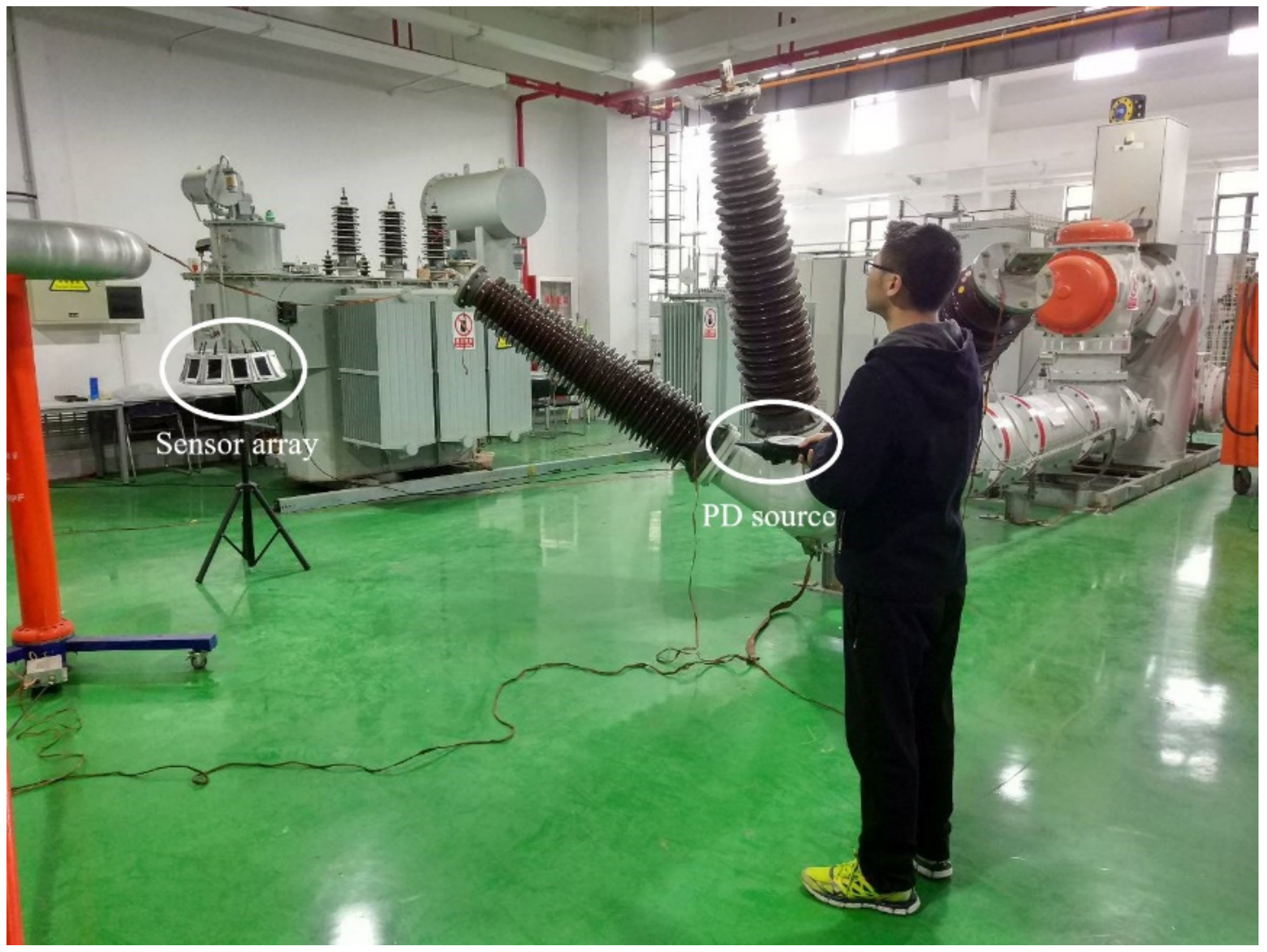
4. Experimental Verification

Experiments were performed in a HV laboratory to verify the effectiveness of the proposed DoA estimation method. The twelve sensors were placed in a circle frame with twelve holes and each sensor was placed in each hole in order. The frame was laid on a tripod. The setup is shown in Figure 8. The PD source was also the EM TEST DITO.

In the experiment test, the azimuth angles of PD were set as 240° and 360° (or 0°) and the distances between the PD simulator and the sensor array were 5 m and 10 m.

In the first situation, the azimuth angle and the distance were 240° and 5 m, respectively. The results after applying the GMM and GPC and the interpolation algorithms are shown in Figure 9 and Figure 10. Thirteen RSSI data are pictured with thirteen black dots and the blue vertical line marks the lowest point of the cubic spline interpolation. In Figure 9, the angle of the lowest point is 57°, and the DoA estimation result is 237°. Also, the polynomial interpolation of the RSSI data is presented in Figure 10. The angle of the lowest point is 50°. The DoA estimation result is 230° for polynomial interpolation.

In the second situation, the distance was longer and set as 10 m. Also, and the azimuth angle was set as the same 240°. The DoA estimation results are shown in Figure 11 and Figure 12. The angle of the lowest point is 67° using cubic spline interpolation in Figure 11 and the DoA estimation result is 247°. The angle of the polynomial interpolation in Figure 12 is 64°. The DoA estimation result is 244° using polynomial interpolation.

In the third situation, the azimuth angle and the distance were set as 360° and 10 m. In the same way, the DoA estimation results are shown in Figure 13 and Figure 14. The angles of the lowest point of cubic spline interpolation and polynomial interpolation are 171° and 188° respectively. The DoA estimation results are 351° and 368° (or 8°), respectively, for cubic spline interpolation and polynomial interpolation.

The details of all three situations’ results can be found in

Table 1. Results of direction of arrival (DoA) estimation.

Azimuth/(°)	Distance/(m)	Preprocess	Interpolation	Result/(°)	Error/(°)
240	5	With GPC	Cubic spline	240.6	0.6
			Polynomial	229.0	11.0
		Without GPC	Cubic spline	240.7	0.7
			Polynomial	229.3	10.7
240	10	With GPC	Cubic spline	235.4	4.6
			Polynomial	230.0	10.0
		Without GPC	Cubic spline	234.5	5.5
			Polynomial	228.7	11.3
360	10	With GPC	Cubic spline	2.7	2.7
			Polynomial	10.0	10.0
		Without GPC	Cubic spline	3.2	3.2
			Polynomial	10.3	10.3

. In the first setup, the DoA estimation results for cubic spline interpolation and polynomial interpolation are 240.6° and 229.0° respectively. The errors are 0.6° and 11.0°. Therefore, at the distance of 5 m, the method using cubic spline interpolation can locate the PD source accurately. Cubic spline interpolation performs better than polynomial interpolation. In the second setup, the DoA estimation results for cubic spline interpolation and polynomial interpolation are 235.4° and 230.0°. The errors are 4.6° and 10.0°, respectively. The error for cubic spline interpolation becomes greater and the error for polynomial interpolation does not change significantly, and the error of the polynomial interpolation is again greater than that of the cubic spline interpolation. The DoA estimation results for cubic spline interpolation and polynomial interpolation are 2.7° and 10.0° in the third setup. The errors are 2.7° and 10.0°, respectively. Overall, the DoA estimation error of cubic spline interpolation is less than 6° while the DoA estimation error of polynomial interpolation is approximately 10°. Moreover, using GPC can improve the location accuracy further.

5. Conclusions

This paper proposes a DoA estimation method for PD based on RSSI and sensor array. Compared to TDoA or ToA techniques, the cost of the proposed method has been reduced by an order of the magnitude without needing a high signal acquisition system. According to [20,21], the errors of DoA estimation using the TDoA or ToA techniques range from 2.4° to 7.2° [6,11]. Also, using RSSI fingerprint localization, the error of angle is about 5° [15]. In the proposed paper, the sensors in the sensor array collect the RSSI data of PD. Then the RSSI data are subjected to GMM, GPC and interpolation algorithms using the specific characteristics of the UHF antenna. The effectiveness of the method has been verified by experiments performed in a HV laboratory. The results show that the average error is less than 5° using a cubic spline interpolation algorithm. The accuracy is approximately the same as with the time delay estimation method, and the low cost and flexibility make our proposal a promising fault early warning system. Furthermore, the DoA estimation of multiple PD sources by the proposed method will be the topic of one of our future works.

References

1. Stone, G.C. Partial discharge diagnostics and electrical equipment insulation condition assessment. IEEE Trans. Dielectr. Electr. Insul. 2005, 12, 891–904. [Google Scholar] [CrossRef]
2. Portugues, I.E.; Moore, P.J.; Glover, I.A.; Johnstone, C.; McKosky, R.H.; Goff, M.B.; van der Zel, L. RF-based partial discharge early warning system for air-insulated substations. IEEE Trans. Power Deliv. 2009, 24, 20–29. [Google Scholar] [CrossRef]
3. Markalous, S.M.; Tenbohlen, S.; Feser, K. Detection and location of partial discharges in power transformers using acoustic and electromagnetic signals. IEEE Trans. Dielectr. Electr. Insul. 2008, 15, 1576–1583. [Google Scholar] [CrossRef]
4. Arefifar, S.A.; Mohamed, Y.A.R.I.; El-Fouly, T.H. Comprehensive operational planning framework for selfhealing control actions in smart distribution grids. IEEE Trans. Power Syst. 2013, 28, 4192–4200. [Google Scholar] [CrossRef]
5. Wang, D.; Du, L.; Yao, C.; Yan, J. UHF PD measurement system with scanning and comparing method. IEEE Trans. Dielectr. Electr. Insul. 2018, 25, 199–206. [Google Scholar] [CrossRef]
6. Tian, Y.; Kawada, M. Simulation on locating partial discharge source occurring on distribution line by estimating the DOA of emitted EM waves. IEEJ Trans. Electr. Electron. Eng. 2012, 7, S6–S13. [Google Scholar] [CrossRef]
7. Portugues, I.E.; Moore, P.J. Study of propagation effects of wideband radiated RF signals from PD activity. In Proceedings of the 2006 IEEE Power Engineering Society General Meeting, Montreal, QC, Canada, 18–22 June 2006. [Google Scholar]
8. Sinaga, H.H.; Phung, B.T.; Blackburn, T.R. Partial discharge localization in transformers using UHF detection method. IEEE Trans. Dielectr. Electr. Insul. 2012, 19, 1891–1900. [Google Scholar] [CrossRef]
9. Siegel, M.; Beltle, M.; Tenbohlen, S.; Coenen, S. Application of UHF sensors for PD measurement at power transformers. IEEE Trans. Dielectr. Electr. Insul. 2017, 24, 331–339. [Google Scholar] [CrossRef]
10. Hou, H.; Sheng, G.; Li, S.; Jiang, X. A Novel Algorithm for Separating Multiple PD Sources in a Substation Based on Spectrum Reconstruction of UHF Signals. IEEE Trans. Power Deliv. 2015, 30, 809–817. [Google Scholar] [CrossRef]
11. Moore, P.J.; Portugues, I.E.; Glover, I.A. Radiometric Location of Partial Discharge Sources on Energized High-Voltage Plant. IEEE Trans. Power Deliv. 2005, 20, 2264–2272. [Google Scholar] [CrossRef]
12. Passafiume, M.; Maddio, S.; Cidronali, A.; Manes, G. Music algorithm for RSSI-based DoA estimation on standard IEEE 802.11/802.15. x systems. World Sci. Eng. Acad. Soc. Trans. Signal Process 2015, 11, 58–68. [Google Scholar]
13. Zhang, Y.; Upton, D.; Jaber, A.; Ahmed, H.; Saeed, B.; Mather, P.; Lazaridis, P.; Mopty, A.; Tachtatzis, C.; Atkinson, R.; et al. Radiometric wireless sensor network monitoring of partial discharge sources in electrical substation. Int. J. Distrib. Sens. Netw. 2015, 11, 1–9. [Google Scholar] [CrossRef]
14. Li, Z.; Luo, L.; Sheng, G.; Liu, Y.; Jiang, X. UHF partial discharge localisation method in substation based on dimension-reduced RSSI fingerprint. IET Gener. Transm. Distrib. 2018, 12, 398–405. [Google Scholar] [CrossRef]
15. Iorkyase, E.T.; Tachtatzis, C.; Atkinson, R.C.; Glover, I.A. Localisation of partial discharge sources using radio fingerprinting technique. In Proceedings of the 2015 Loughborough Antennas & Propagation Conference (LAPC), Loughborough, UK, 2–3 November 2015. [Google Scholar]
16. Li, Z.; Luo, L.; Liu, Y.; Sheng, G.; Jiang, X.P. UHF partial discharge localization algorithm based on compressed sensing. IEEE Trans. Dielectr. Electr. Insul. 2018, 25, 21–29. [Google Scholar] [CrossRef]
17. DITO ESD SIMULATOR Data Sheet. Available online: www.emtest.com/products/product/135120100000010183.pdf (accessed on 21 July 2019).
18. Xu, J.; Liu, W.; Lang, F.; Zhang, Y.; Wang, C. Distance measurement model based on RSSI in WSN. Wirel. Sens. Netw. 2010, 2, 606–611. [Google Scholar] [CrossRef]
19. Biernacki, C.; Celeux, G.; Govaert, G. Assessing a mixture model for clustering with the integrated completed likelihood. IEEE Trans. Pattern Anal. Mach. Intell. 2000, 22, 719–725. [Google Scholar] [CrossRef]
20. Rasmussen, C.E.; Nickisch, H. Gaussian processes for machine learning (GPML) toolbox. J. Mach. Learn. Res. 2010, 11, 3011–3015. [Google Scholar]
21. Neal, R.M. Bayesian Learning for Neural Networks; Springer Science & Business Media: New York, NY, USA, 1996. [Google Scholar]
Figure 1. Designed ultra-high frequency (UHF) antenna: (a) diagram of antenna structure; (b) picture of printed circuit board (PCB) antenna; (c) radiation pattern at 1100 MHz.
Energies 12 03450 g001
Figure 2. Designed wireless UHF Sensor: (a) diagram of wireless UHF sensor; (b) picture of wireless UHF sensor.
Energies 12 03450 g002
Figure 3. UHF sensor array radiation pattern.
Energies 12 03450 g003
Figure 4. Collected raw partial discharge (PD) UHF received signal strength indicator (RSSI) measurements along a 20 m range. (a) LOS conditions; (b) NLOS conditions
Energies 12 03450 g004
Figure 5. The decision curves learned by a Gaussian process classifier (GPC) using collected PD line of sight (LOS)/ no-line of sight (NLOS) measurements.
Energies 12 03450 g005
Figure 6. UHF antenna power pattern: (a) Side view; (b) Top view.
Energies 12 03450 g006
Figure 7. Flow chart of the proposed direction of arrival (DoA) estimation method.
Energies 12 03450 g007
Figure 8. Sensor array in the high voltage (HV) laboratory.
Energies 12 03450 g008
Figure 9. Diagram of cubic spline interpolation.
Energies 12 03450 g009
Figure 10. Diagram of polynomial interpolation.
Energies 12 03450 g010
Figure 11. Diagram of cubic spline interpolation.
Energies 12 03450 g011
Figure 12. Diagram of polynomial interpolation.
Energies 12 03450 g012
Figure 13. Diagram of cubic spline interpolation.
Energies 12 03450 g013
Figure 14. Diagram of polynomial interpolation.
Energies 12 03450 g014