A Process to Implement an Artificial Neural Network and Association Rules Techniques to Improve Asset Performance and Energy Efficiency

Abstract

In this paper, we address the problem of asset performance monitoring, with the intention of both detecting any potential reliability problem and predicting any loss of energy consumption efficiency. This is an important concern for many industries and utilities with very intensive capitalization in very long-lasting assets. To overcome this problem, in this paper we propose an approach to combine an Artificial Neural Network (ANN) with Data Mining (DM) tools, specifically with Association Rule (AR) Mining. The combination of these two techniques can now be done using software which can handle large volumes of data (big data), but the process still needs to ensure that the required amount of data will be available during the assets’ life cycle and that its quality is acceptable. The combination of these two techniques in the proposed sequence differs from previous works found in the literature, giving researchers new options to face the problem. Practical implementation of the proposed approach may lead to novel predictive maintenance models (emerging predictive analytics) that may detect with unprecedented precision any asset’s lack of performance and help manage assets’ O&M accordingly. The approach is illustrated using specific examples where asset performance monitoring is rather complex under normal operational conditions.

1. Introduction

Nowadays we are living a digital transformation in maintenance and asset management, characterized by higher assets’ performance information levels and enhanced management control possibilities, in real time and throughout the useful life of the assets.

Data is what really enables this transformation and is becoming critical in today’s organizations [1]. Having useful data available is becoming paramount in order to be able to make the best decisions in Asset Management (AM). However, transforming data into information and the management of this information as knowledge are still challenges. Different researchers agree in the fact that an integrated asset information management strategy is required [2] in order to effectively habilitate the AM decision-making.

Besides the long-term availability of data, the quality of decisions made is often constrained by the quality of data available. Thus, data quality is another interesting and recent topic for research for asset management practitioners [3]. Therefore, research has also focused on developing frameworks for assessing and improving data availability and quality.

When considering which data are needed for supporting informed AM decision-making, the required data can vary from case to case. The major challenge is that required data is usually scattered among separate information systems (Enterprise Resource Planning systems (ERP) and other external information sources that have not been integrated, and other non-automatic sources) [4,5]. As widely agreed, integration should facilitate the bidirectional data and information flows into the decision-making process at all levels [4] of asset control. The basic concept is the need for a common asset database to provide a primary reference to information regarding assets’ properties for supporting decisions [5].

Another key development to improve data quality and long-term availability is the emergence of digital technologies and their adoption in AM. In this regard, Internet of Things (IoT) [6,7,8] and Cyber-Physical System (CPS) [9] are currently leading concepts of the transformative process pushed by a blend of mature technologies. Big Data analytics, that access the data and promise to provide fast decision-making with the use of smart analytics tools [10,11], are in fact going to complement the IoT with further features useful for decision-making support.

The growing data availability enabled by Industry 4.0 technologies makes the traditional techniques for data analysis obsolete. Indeed, to deal with such an amount of data, the application of appropriate algorithms for data understanding and knowledge extraction is necessary. In this context, an important contribution is provided by Knowledge Discovery in Databases (KDD) techniques: analyzing a massive amount of data, KDD’s goal is to extract useful information and derive knowledge [12,13]. Data Mining (DM) techniques belong to the KDD domain and, according to [14], they regard the discovery of hidden information and patterns, as well as relationships in large databases [15]. Advanced simulation will also play a key role, amongst the tools relevant for prediction of the stochastic processes that occur in the physical world [16].

Finally, in such a technology landscape, an important concept is often noted, that is the Digital Twin (DT), considered as a virtual entity, relying on the sensed and transmitted data of the IoT infrastructure, as well as on the capability to elaborate data through data analytics and simulation technologies, with the purpose to allow optimizations and informed decision-making. The potentials for decision support along the asset lifecycle offered by DT modeling are highly promising, leading to think of future applications built on the DTs of Physical Assets.

Problem Description

In this paper, we address the problem of assets’ performance monitoring, with the intention of both detecting any potential reliability problems and predicting any loss of energy consumption efficiency.

The idea of the paper is to add new capabilities to existing Condition-Based Maintenance (CBM) programs that may exist in energy plants and facilities. CBM is defined as “Preventive maintenance including a combination of condition monitoring and/or inspection and/or testing, analysis and subsequent maintenance actions” [17]. CBM monitors the condition of maintainable items in order to dynamically determine a suitable preventive schedule [18]. ISO 13372 [19] defines CBM as “Maintenance performed as governed by condition monitoring programs”.

CBM can be presented in the literature as a system, program or solution. For instance, the US Army [20] defines the “CBM system” as a system including the analytical methods, sensors, data acquisition (DA) hardware, signal processing software, and data management standards necessary to support the use of CBM as a maintenance approach to sustain and maintain systems, subsystems, and components. A “CBM program” comprises the application of the different CBM solutions that have been adopted for a particular system involving management and maintenance task planning [21]. A “CBM solution” can be understood as the application of a particular monitoring solution to a specific case (failure mode or element).

CBM is increasingly becoming common in engineered systems. In recent decades, we have seen the transition from maintenance approaches that combine run-to-fail and programmed preventive maintenance to more efficient maintenance approaches such CBM [22]. As instrumentation and information systems become cheaper and more reliable, CBM becomes an important tool for running a plant or a factory [18]. In automated manufacturing or process plants, condition-based maintenance (CBM) is preferred wherever it is technically feasible and financially viable [23].

Condition monitoring techniques such as vibration analysis, thermography, acoustic emission or tribology [19], along with developments in Prognosis and Health Management (PHM) has provided new powerful capabilities for maintenance [24,25]. These capabilities allow us to treat, efficiently, the new maintenance challenges in modern systems and applications [20,26].

However, the problem of asset’s performance monitoring can become a very complex problem in some operational situations when:

• The assets can perform in very diverse operating conditions (sometimes also diverse environmental conditions) over time;
• Assets’ condition is not feasible to be monitored, or simply doing it becomes a complex technical problem with a very troublesome and economically non-viable solution. This difficulty many times related to the asset specific functional location;
• Altogether could cause a lack of assets performance control and subsequent loss of expected performance efficiency.

To overcome these problems, we need practical tools that can be adapted to any potential current asset location and operating condition, having the possibility to control asset performance and reliability, ensuring life cycle expectations according to existing business plans.

This has become an important concern for many industries and utilities with very intensive capitalization in long-lasting assets [27]. These organizations demand innovative, practical solutions, that can somehow replicate the benefit provided by emerging IoT and CPS, but in currently existing assets, contributing to their current assets’ Total Cost of Ownership (TCO) and/or Total Value of Ownership (TVO) [28], the latter in case that we can somehow model, and quantify, the value provided by the asset along its life cycle.

To this end, we will first introduce ANN and DM techniques that will be used in the paper. ANN will be proposed to solve the problem of identifying when asset behavior abnormalities appear while DM AR techniques will be used to in detail for which operating conditions are appreciated as behavior abnormalities, and to what extent is energy efficiency impacted. Then we will present the proposed process, together with some samples to appreciate the way its implementation is deployed. Finally, we present some practical results, conclusions and further research opportunities.

2. Rational for the ANN and DM Techniques Selection

Within the AI tools, Artificial Neural Networks (ANN) is the tool selected because of their ability to process information features in non-linear, high-parallelism, fault and noise environments with learning and generalization capabilities [29,30]. In comparison to other methods, ANNs are well suited for solving problems where explicit knowledge is difficult to specify or define, but where there are enough data [31,32]. For these reasons ANN are a very popular tool for prediction and classification problems, but we agree that more research is needed to make their implementation more practical in real life applications, taking advantage of existing maintenance engineering tools and management systems [33].

Concerning data analysis tools, several DM techniques exist and, according to the purpose of each study and to the characteristics of the variables under investigation, the accurate selection of the most appropriate one is the first step for the success of the analysis [34]. We propose a classification of the DM techniques, differentiating among models requiring or not a reference value for the analyzed variable. The former group is furtherly detailed, discriminating between descriptive models, namely the ones oriented to defining relationships among objects (e.g., conceptual clustering), and associative models, addressing the relationships among variables (e.g., association rules, model-based reasoning, reason weighting). According to this, among the DM techniques, we selected Association Rules (ARs) mining for two main reasons: firstly, because of its purpose, that is discovering relevant and non-trivial attribute-value relations not immediately recognizable in a massive amount of data [35]. The second one is related to ARs’ mining intuitiveness, that makes results interpretation instantaneous even for non-domain experts. Also, ARs mining is very popular in several different fields of application.

In this paper, we will propose an innovative process for determining the proper combination of ANN tools with Data Mining (DM) techniques. In fact, the combination of these two techniques can now be done using software which can handle large volumes of data (big data), assuming that the data must be available during the asset’s life cycle, and that its quality must be tested. If this process could be practically implemented, novel predictive maintenance models may emerge (predictive analytics), models that with unprecedented precision may detect any asset lack of performance and therefore help to manage asset O&M.

2.1. State of the Art: ANNs Applications in AM

As already mentioned, ANNs represent a powerful methodology for prediction and classification issues. Specifically, they enable condition analysis of the asset and of the operating variables, with the aim of anticipating potential problems [36].

In the existing literature, there are several applications of ANNs referring to predictive maintenance and asset management. For instance, [37] studied the condition of gearbox bearings in wind turbines using a nonlinear autoregressive ANN, in order to estimate their condition and anticipate possible failures. Moreover, ANNs can be combined with other techniques, like decision trees, in order to improve the accuracy of the prediction obtained: an example of this combination is presented for the maintenance of heating ventilating and air conditioning systems [38] or in engine gearbox fault diagnosis [39]. ANNs have also been applied to detect the health status of rotatory components; an enhancement of the ANN’s learning stage (e.g., reducing the calculation time) can be performed by estimating weights and biases through a Genetic Algorithm, as suggested by [40]. In [41], an asset prognostic system, based on principal component analysis and back-propagation ANN, is proposed and applied to transformers of a large power system. The potentiality of ANNs in fault diagnosis is proven, among the others, by [42] that analyzed the vibration data to predict bearings failures, while [43] addressed the engine cylinders temperature to foresee potential malfunctioning. A similar approach is also applied for controlling the exhaust gas temperature of gas turbine engine and detecting wearing problems: integrating data recorded through different sensors of the turbine, allows the monitoring of the turbine’s performance and fault detection [44]. Another application belonging to the energy field regards the analysis of temperature and irradiance values to predict the performance and failures of photovoltaic plants [45]; interestingly, as implemented in a power grid company, ANNs may also be integrated in ontological models to optimize the faults diagnostics and repairing processes [46].

The ANN technique can be considered therefore a mature technique with high technological readiness for its immediate implementation and in many companies many different applications where they are used can be found. This makes rather practical the implementation of ANN algorithms for prediction in many industrial scenarios, of course given the accuracy and fitting of the algorithm is the appropriate one.

2.2. State of the Art: AR Mining Applications in AM

ARs were first applied to determine the relationships among items frequently bought together [47]. With the growing popularity of such a methodology, the applications to other fields increased as well, furtherly highlighting the versatility of the methodology. For example, in the manufacturing field, ARs mining is applied for relating the root cause to groups of machines in a production process [48] or in predicting process failures [49,50].

Other ARs mining applications regard the analysis of events co-occurrences or correlations. For instance, they can be used in defining the occurrence of couples of events, as presented in case of trains diagnostics [51]: rules relating sequential events are taken into consideration, in order to more efficiently monitor train fleets. In a similar manner, process reliability and safety is addressed by several authors: [52] develop a procedure for failure detection on machines belonging to different production lines, by integrating maintenance data; [53], instead, apply the ARs to deploy a Total Productive Maintenance strategy to increase the reliability of the production process. Maintenance policies based on ARs mining for the prediction of components’ breakages are also applied in existing contributions related to refinery plants, both involving an active participation of plants operating personnel in parameters setting [54] and automatizing the latter aspect through the resolution of an optimization model considering production constraints [55]. Conversely, some authors showed that the application of ARs mining in power plants has a positive impact for diagnostic purposes, but are not a sufficient in predicting failure occurrences [56].

The ANNs and ARs mining approaches are promising methodologies for prediction and classification, but more research is needed in terms of combination of the two. A work integrating the ARs mining and ANNs approaches operational reliability issues is already existing in literature: specifically, the ARs are extracted to define the factors influencing power distribution reliability; then, such factors are given in input to an ANN for the normal behavior modelling of the distribution net [57]. The approach proposed in the current paper is the opposite: indeed, the normal behavior is firstly estimated through an ANN and, when a substantial deviation is noticed, the ARs mining is applied to diagnose whether such a deviation impacts on the efficiency and performance of the asset. In fact, if the ability of ANN models to predict the normal behavior of a system starting from the analysis of the process’ variables is indisputable, it might also be useful to understand what are the impact that influence the abnormal behaviors of the process. Such an analysis can be easily carried out through the ARs mining. For this reason, the approach proposed in the current paper regards the combination of the ANN and ARs mining.

3. Brief Background of the ANN-DM Techniques Selected

The ANN architecture selected consists of an input layer, an output layer and one or more hidden layers. Research has been made in evaluating the number hidden layers (deep of the network) and the number of neurons in these layers, normally depending on the problem complexity or on the accuracy needed [58]. Also, neural networks may use different available training algorithms to learn from data, with different features and efficiency [59]. The learning process consists of an iterative process to minimize a function (named loss function), which is normally a non-linear function containing the ANN parameters (biases, learning rate and weights). The process stops when a specified condition is reached.

In the literature, we can find many different training algorithms among which the gradient descent is recognized as the simplest one [60]. This is a first order method that will be used in this paper to implement a backpropagation process to train the network so that the ANN can learn to link arbitrary inputs to outputs. The backpropagation algorithm has been selected since it has provided excellent results compared to conventional lineal and polynomial methods dealing with time series of data [61].

In this paper, the ANN with backpropagation prediction model selected is a continuous time simulation model that has demonstrated to be easy to adapt for prediction accuracy and self-learning capabilities (as explained later in Section 4.2).

Concerning our data analysis tool, once the current study addresses the identification of the relationships among variables, an associative model is required and, specifically, the Association Rules (ARs) are mined. A formal definition of an Association Rule and a description of the rule mining algorithm is provided in the following.

Given a set of Boolean data I = {i1, i2, … in} called items and a set of transactions T = {t1, t2, … tm}, a transaction ti is defined as a subset of items belonging to I (i.e., an item-set). An Association Rule (AR) is an implication in the form Γ → Δ, where Γ and Δ are item-sets belonging to I and whose intersection is null (i.e., Γ ∩ Δ = Ø). Γ and Δ referred to as body and head of the rule, respectively. The quality of an AR can be assessed through different metrics; in this study, we apply the most popular ones, that are (1) the Support and (2) the Confidence.

(1) Support (Γ → Δ) = (|Γ,Δ|)/m: the support is the ratio between the number of transactions both containing the item-sets Γ and Δ (|Γ, Δ|) and the total number of transactions (m). Hence, it represents the probability of finding a transaction containing Γ and Δ.

(2) Confidence (Γ → Δ) = (Support(Γ → Δ))/(Support(Γ)): the confidence can be considered as a measure of the strength of the rule. Indeed, it is calculated as the support of Γ → Δ over the support of item-set Γ. In practice, confidence represents the probability of occurrence of Δ, given the occurrence of Γ, i.e., the conditional probability of Δ, given Γ.

The procedure for mining the ARs from a dataset, starts from the generation of the Frequent Item-sets: the users define a minimum support according to the dataset’s characteristics; then, the item-sets appearing in T with a frequency higher than the minimum support are generated through the FP-growth algorithm [62]. Starting from each frequent item-set F, all the rules in form X → Y, such that X U Y = F, are generated.

Since assets’ performance monitoring involves the analysis of continuous variables, the discretization of such attributes should be taken into account. This issue is already addressed in existing literature: indeed, some authors provided guidelines on how discretizing such values. For example, [12] propose an entropy minimization-based heuristic to define multiple intervals, while [63] propose the application of an evolutionary algorithm to define ranges automatically. Data could also be clustered before extracting the ARs, even if some relationships can be disregarded (e.g., the support of such rules does not reach the minimum support required). In order not to lose any relevant information, in the energy consumption monitoring field, data are often partitioned according to a specific strategy, e.g., in fixed ranges [64]. Hence, in our application, the discretization of the continuous variables is defined in accordance with the O&M department, so that all the different operating conditions can be mapped. The software RapidMiner (www.rapidminer.com), an opensource data mining platform, is selected to carry out the analysis. Among the various tools available on the market, RapidMiner is being considered one of the most user-friendly, because of the graphical interface and the ease of modifying the parameters, since no programming skills are required [65].

4. ANN-DM Combination Process and Sample Problem

The “Asset Performance Monitoring and Reliability Assessment Process” coordinates and integrates data, engineering tools and human resources (with knowledge, skills and experience) in order to achieve the best possible recommendation for assets’ operations and maintenance actions. This process also analyzes the different renovation and reinvestments options which are available for the physical asset. All these activities are accomplished taking into account different operational and data related constraints and controls, as presented using the Functional Modelling method IDEFØ diagram [66] of the process in Figure 1.

This process is a continuous improvement process responsible for leading and controlling the knowledge captured concerning the behavior of the asset (observed properly when integrating O&M Data [I1], with process [I2] and condition monitoring data [I3]), adapting permanently operations and maintenance actions. The process provides consistency to major maintenance actions and assets replacement options ensuring proper AM orientation according to predictable and/or unpredictable circumstances that may take place.

The general process in Figure 1 can be split into four different subprocesses, named modules in this paper, as illustrated in Figure 2. The first module is Data Processing, responsible for the preparation of valid data, quality tested (O1), for the subsequent processes, as well as for the normalization of this data (O2). The second module is the one to provide an algorithm that can identify deviations of the asset from its expected behavior under normal operating conditions. These deviations are presented in the form of prediction error (O3). The third module deals with the measurement of the deviation, obtaining the relationship between operational data and efficiency (O5) and then calculating the efficiency loss observed for a period (O6). Finally, the last module takes this information to adjust O&M actions properly (O7) and to reevaluate asset major interventions (O8) accordingly.

In the following paragraphs, we explain each one of these processes with detail, going down to level 2 in the IDEFØ diagram presented (therefore we use the Functional Modeling method IDEFØ with three hierarchical series of diagrams). In addition, the application of each phase of the process is illustrated with a practical example.

4.1. Sample Problem Description

For this paper we have selected the example of a process pump located inside a cryogenic LNG storage tank, with the following features:

• A unique design allowing the pump to be installed inside the tank in a vertical column to remove the possibility of major tank leakage due to a pipe or connection problem.
• The pump and motor units are submerged, and the column acts as a guide to seat the pump during installation and performs as the discharge pipe from the pump.
• The plant information system shows operating conditions of the pump to detect any potential problem.
• The pump has very different possible operating conditions (resulting of very different tank levels, flow, pressure, LNG density, operating hours of the pump, etc.).
• It is very troublesome to establish a clear judgement about potential pump malfunctioning. Besides this, condition monitoring capabilities are limited to previously mention operating variables (for instance, no items vibration, bearing temperatures, motor temperatures are received).

In this example, the scope of the analysis was fixed as follows:

• To generate a process and tool for the prediction of anomalies in the operation of the pumps with complex operation and supervision regime.
• To establish the guidelines for the practical implementation of the models and methodology.
• To generate enough information to prepare a Business Case for the company to implement the process if there is a demonstrated payback to the business.
• Some other secondary or complementary objectives were:
• To identify the operating regimes of the equipment so that anomalies are recorded.
• To obtain the loss of performance of the equipment when producing the anomalies detected.

4.2. Imput Data Processing Module

The procedure described below is necessary to unify the data received from different information sources. For this, the guidelines for data capture, cleanup and subsequent standardization are listed. In this way, we can ensure that ANN models and association rules are as effective and precise as possible.

The steps listed below are shown in detail in the IDEFØ 1.1 to 1.5 diagram (Figure 3):

(1)

Asset case study definition: The first step of the procedure (IDEFØ1.1) is to choose the asset case study from organization asset portfolio (I1.1) so that it can be representative to extend the results to other similar equipment or systems of the plant. For the equipment selection, the organization must have good and consistent data for operation and maintenance history (C1.1) that allows obtaining the model of the same with success. In this step, it is convenient to collect all the technical information of the equipment (C1.3), referring to the maintenance and operation recommendations by the manufacturer. Each operation variable that is extracted from the control system of the equipment will have to be standardized based on the design standards. Additionally, another restriction to consider is the operational context, to understand how the equipment works in their environment and how they can be affected by external conditions and different modes of operation (C1.2). Singular case studies and the obtaining of a single model for single equipment can be given, or alternatively, the option of a sufficiently flexible model to be able to extend to similar equipment, and in this way, take advantage of the work and the dedicated effort. In many cases, the operational context may be completely different, because of location, altitude, external agents and other operational parameters that accelerate ageing and variation of performance. So, it is advisable to choose equipment that do not have the same operational context to obtain better accuracy in obtaining the model. The final decision to select the asset case study is approved by O&M Manager “R2”, based on the above comments. The following table shows all available variables and the origin of them (

Table 1. Asset case study definition, data source, for the process pump example.

Variable	Corrective & Preventive Maintenance	Fluid Density	Flow	Intake Temperature & Output Temperature	Output Pressure	Tank Level	Power Consumption	Operation Modes	Hours Since Last Overhaul
GMAO	√
LNG Quality Registration		√
Plant Information System			√	√	√	√	√
Shift superintendent book								√
Pump horometers									√

):

(2)

Selection of variables: Once the case study equipment has been chosen and the operational context described, as indicated in the previous paragraphs, the next step (IDEFØ 1.2) is to select the variables that are used for modeling and studying the behavior by ANN and association rules. All the variables must be part of the historical operation and maintenance, and to comply with the following requirements:

• Data must be consistent and without significant temporal breaks in the series.
• The frequency at which the information is extracted from different sources of information must be enough to capture the changes of state in each of the variables.
• The variables must be independent of each other, if some dependencies between variables are detected, those dependent variables for which less information is available will be discarded.
• At least one or more variable must be of operation (for example, flow, pressure, electric consumption, power consumed, speed, etc.).
• The other variables must be linked to the equipment condition, such as vibration, bearing temperature, etc. In addition, some variable must be related to the operational context and environment, such as outside temperature, required load, operation mode, etc.

Notice that in order to improve the choice of variables, it is advisable to use statistical techniques to measure the degree of dependence (see R1 in previous Figures). For the example presented in this paper, the variables that have been selected and that will follow the next phases of the process are those shown in

Table 2. Sample covariance matrix and correlation coefficients, to identify the dependence between variables.

COVARIANCE	Flow	Output Pressure	Power Consumption	Intake Temperature	Output Temperature	Tank Level	Fluid Density	Hours Since Last Overhaul
Flow	0.04100
Output pressure	−0.01438	0.01096
Power consumption	0.03624	−0.01337	0.03503
Intake temperature	−0.00531	−0.00167	−0.00562	0.014173
Output temperature	−0.01038	0.00208	−0.01078	0.00905	0.02344
Tank level	0.00565	0.00538	0.00543	−0.01025	−0.00348	0.02418
Fluid density	−0.00457	0.00241	−0.00281	−0.00077	−0.00340	−0.00315	0.01663
Hrs since last overhaul	−0.00844	0.00100	−0.00922	0.00279	0.00428	−0.00392	0.01136	0.08351

.

This table is the result of applying statistical techniques; in particular, it has been studied using a covariance matrix and correlation coefficients, the dependence between variables [67]. The analysis of the results assumes that flow, output pressure, output temperature and Hrs since last overhaul are indispensable for the model, and that other variables such as fluid density, tank level and intake temperature are secondary, and they could be left out of the model if sufficient data is not available for power consumption prediction modeling.

(3)

Period selection and data recording frequency: Once the variables have been selected, it is necessary to define the period in which the study will be carried out (IDEFØ 1.3). It is advisable to choose a period in which all possible scenarios have been registered, for example, that the system has operated in all different operating modes, overhauls, corrective maintenance, etc. Likewise, in addition to selecting the period, it is also necessary to select the interval of data recording of the different information sources. As mentioned in step 2, this period must allow us to capture with enough detail, the change of state in the variables for its interpretation and study, with the objective of training the network faithfully and being able to identify anomalies in the behavior of the equipment (C1.4). At this point, it is convenient to carry out a study between the efforts required to obtain the data and the subsequent results for a model with a high level of precision. For a shorter sampling interval, higher levels of accuracy in the prediction of the model are obtained (for example, data/minute vs data/hours). In

Table 3. Period selection.

Hours	Period before OH 1		Period before OH 2		Period before OH 3
Operating hours	From 2.375	To 16.147	From 0	To 5.173	From 0	To 94
Valid data points	10.082		4.857		49

, the periods selected for the case study are shown. It is divided into three periods; the passage from one period to another is marked by an overhaul (OH) maintenance activity. The data recording frequency has been every calendar hour.

(4)

Data validation and processing: This step involves the validation and processing of the information (IDEFØ 1.4). This is one of the most important steps and usually the one that consumes more resources in the application of the methodology. Usually, there are errors in the information that must be reviewed and above all, the unification of the information from the different information sources in the same selected period. The importance of this step is essential to achieve results that are as close as possible to reality. Another measure to consider at this point is the revision of the consistency of the database, filtering the noise and erroneous information generated by the instrumentation installed in the assets. For this, it is necessary to use data validation tools “R1”, representations by dispersion diagrams, etc. Once the data has been normalized, the next step is the implementation in the artificial neural network to obtain the ideal model of system behavior. The model obtained, together with the real-time reading of the variables, can be compared with the real behavior of the system, so that in an ideal case, the deviation from the expected behavior can be detected.

(5)

Data normalization: Normalization is applied as part of data preparation for machine learning (IDEFØ 1.5). The goal of normalization is to change the values of different variables in the dataset to a common scale, without distorting differences in the ranges of values. For machine learning, every dataset does not require normalization. It is required only when features have different ranges. Each variable is normalized between 0 and 1, making use of the technical information collected in the first step of the procedure. For example, if a variable is by design limited between 250 and 700 m³/h, the values that are outside the range are not considered for the study, but the values within the range will be normalized between 0 for values close to 250 m³/h and 1 for values close to 700 m³/h. In the following table, the maximum (Vmax) and minimum (Vmin) values for each of the variables selected for the case study are shown in

Table 4. Values for data normalization.

Variable	Vmin	Vmax
Flow (m3/h)	250	700
Intake Pressure (kgf/cm2)	6	14
Intake Temperature (TAsp) (°C)	−160.5	−150
Impulsion Temperature (TImp) (°C)	−160.5	−153.5
Tank Level (Nivel T) (mm)	0	50,000
LNG Density (Dens GNL) (kg/m3)	430	465
Hrs since last Overhaul (h)	0	16.128
Power (Kwh)	200	350

.

4.3. Prediction Model Module

As mentioned above, in this paper, the prediction model selected is a continuous time simulation model that has demonstrated to be easy to adapt for prediction accuracy and self-learning capabilities. The model (Figure 4) implements an ANN with a backpropagation algorithm using Vensim^® simulation environment (Ventana Systems Inc., Harvard, MA, USA), to benefit of the outstanding software optimization features for fast training. The stock and flow diagram—SFD—of the simulation-based prediction model is presented in Figure 5.

Besides providing high rigor for writing model equations, Vensim helps to trace and to understand the importance of model existing feedback loops and supports multiparametric optimization that will result essential for this process (IDEFØ 2.1 in Figure 4). Some interesting features of the model that has been implemented in this process are:

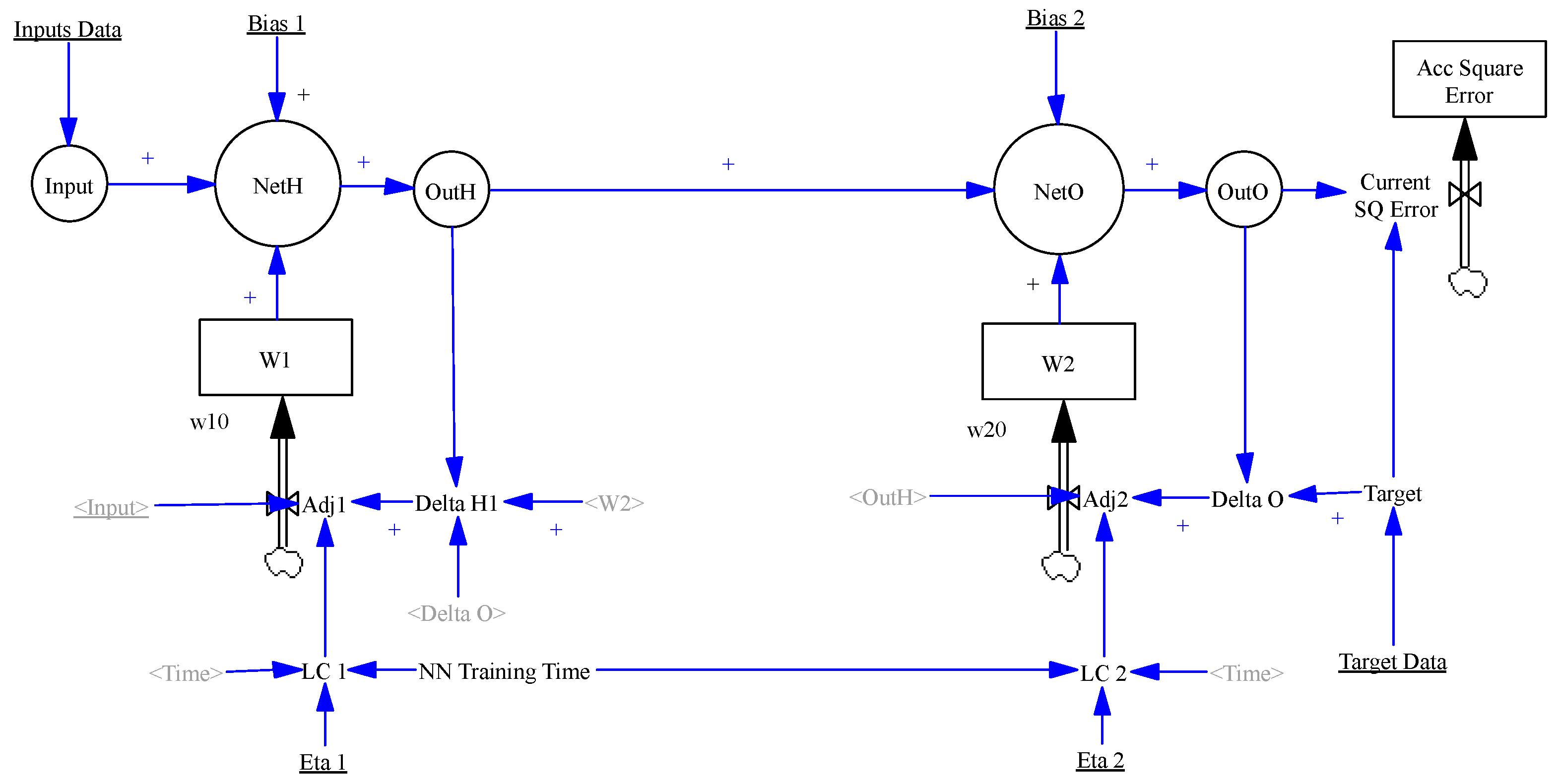
• The ANN structure (number of neurons per layer) can be easily changed by modifying the number of elements of the different subscripts, which correspond to the number of neurons of the network (in our initial model we have considered only one hidden layer and 20 neurons).
• The network has two bias parameter (hidden layer [Bias 1] and output layer [Bias 2]) and two learning coefficients or rates (hidden layer [LC 1 = Eta 1 during training time] and output layer [LC 2 = Eta 2 during training time]).
• Input Data (in our example values of flow, temperatures, tank levels, densities, and operating hours, to predict a pump energy consumption) and target data (values of energy consumption) are imported from plant information systems, to be uploaded automatically to Vensim (O2 in Figure 4). Input data goes to first layer neurons, while target data will be compared with the values predicted by the ANN output.
• ANN Training time is introduced as a parameter, once this time is reached in the simulation, the LC1 and LC2 are set to zero, and the learning process finished since the adjustments flows of the weights will be stopped.

To overcome potential training dynamic issues, we can rely on tools provided by Vensim for optimization and calibration of model parameters. Vensim uses the direct-search method that does not evaluate the gradient (Powell Modified Method), to calibrate model parameters [68,69] In our case, it is important to calibrate Bias 1, Bias 2, Eta1 and Eta2 (learning coefficients), and all initial weights parameters w1o(i,j) and w2o(j,k) in order that the ANN offers its best possible fit as soon as possible. The optimization model implemented in the Vensim Powell Optimizer in our (IDEFØ 2.1) is as follows:

Objective Function:

Min ∑t Current SQ Error t

with t = 1 … Final Simulation Time

Subject to:

−1 ≤ w10(i,j) ≤ 1	with i = 1 … n inputs, j = 1 … m neurons in the HL
−1 ≤ w20(j) ≤ 1	with j = 1 … m neurons in the HL
0 < Eta 1 ≤ 1	For the leaning coefficient of the HL
0 < Eta 2 ≤ 1	For the leaning coefficient of the Output Layer
BMin < Bias 1 ≤ BMax	with BMin y BMax to be selected (for instance −10, 10)
BMin < Bias 2 ≤ BMax	with BMin y BMax to be selected (for instance −10, 10)

where w₁₀ (i, j) and w₂₀ (j, k) are the initial weights values.

With Vensim the analyst can select to stop the algorithm according to a maximum number of iterations or according to certain tolerance criteria for the solution. It is surprising to see the low error obtained for a relatively few number of iterations of the algorithm. Once the optimization algorithm is stopped, results for parameter values can be logged together with the performance of the model for the optimal solution found.

Proceeding in this way, we can easily select initial model parameter values, and then by running the model with the backpropagation algorithm, we can obtain final weights values for the ANN algorithm that will be put into operation (IDEFØ 2.3 in Figure 4).

For our pump example, the considered ANN model structure, where the authors had to initially iterate five times with the number of neurons in the hidden layer, can be characterized as:

• Three layers
• Seven neurons in the input layer
• Twenty neurons in the hidden layer (previously tested between 5, 10, 15, 20 and 25)
• One output neuron

The implementation in Vensim required:

(1)

Connection with standard data in Excel provided by Plant Info Systems;

(2)

Training interval definition (first 70% of valid data points in Table 3, Period 1, in chronological order);

(3)

Basic tests of operation and validation of the ANN Model;

(4)

Optimization of ANN algorithm values optimizing a total of 164 parameters:

• Initial weight values w₁ (i, j), i = 7, j = 20; 140 parameters
• Initial weight values w₂ (j), j = 20; 20 parameters
• Parameters Bias 1 and Bias 2; 2 parameters
• Learning Coefficient Eta 1 and Eta 2; 2 parameters

(5)

Simulation with the backpropagation algorithm to find the final values for:

• Weight values w₁ (i, j), i = 7, j = 20; 140 parameters
• Weight values w₂ (j), j = 20; 20 parameters

(6)

The testing (30% remaining of valid data points in Table 3, Period 1, in chronological order) and calculation of the quadratic error of prediction;

(7)

The prediction error trend study.

Results of the prediction error (as in Figure 6) provide precise information about possible abnormal operating conditions of the assets for any operating regime (or, as in Figure 6, after an overhaul intervention carried out on the asset). Calibration can be done for each network configuration selection (i.e. given numbers of neurons per layers: n, m, l), and each time input data conditions recommend to retrain the network.

Sample additional regression results for the ANN algorithm (for the 20 neurons in the hidden layer) are presented in

Table 5. Artificial Neural Network (ANN) algorithm results for the regression problem (with 20 N/HL).

Metric	Training	Before the Overhaul 1	After the Overhaul 1
RMSE	0.00030	0.00043	0.00222
MAE	0.01567	0.02297	0.05447
MAPE	0.02807	0.03963	0.12195

. Notice how step 4 of the Vensim model implementation process, described above, provides extremely good results for training (Table 5) since all initial values for the weights, biases values as well as training coefficient are already optimized when the backpropagation algorithm starts for the final run with optimal parameter values. Therefore, the backpropagation algorithm just refines the values for the weights set by the direct search technique.

The precision of the algorithm results can be observed in Figure 7, where a histogram of absolute values for the results of prediction before the overhaul of the pump is presented.

Therefore, by using the Vensim model and software, the algorithm to put into operation (final ANN model) will be the result of two optimization phases:

(1)

Direct search techniques using the modified Powell method applied for the optimization of initial values of weights, biases and learning rate coefficients (in IDEFØ 2.1. in Figure 4).

(2)

Backpropagation algorithm for the optimization of the weights during the ANN training period (IDEFØ 2.2. in Figure 3), when we use initial values of weights, biases and learning rate coefficients optimized in IDEFØ 2.1.

Before concluding this phase and regardless of the fact our results are promising, we realize that the selection of a given technique, like ANN, should not be done without discussing whether we are delivering results that can be benchmarked to those provided by other available advanced machine learning techniques for predictive analytics. This certainly supports the tool selection and provides more elements for a well-informed decision for the management of assets [33].

It is important to say that not all the techniques that we will now review have the same maturity level than ANNs in reliability analysis or maintenance. For instance, we have few examples of Support Vector Machines (SVM) or Random Forest (RF) to predict systems performance and reliability, the utilization of these techniques, in the referred fields, will probably take place with more intensity in the coming years [70].

Regarding the application of SVM techniques compared to ANN, the readers are referred to [71] where a study is presented comparing different Neural Network techniques (NNBR, NRBR, NRBR) and NSRV, based on the results obtained in each of them from the mean square error and the relative mean (RMSE and MRE). This model of artificial intelligence (SVM) is in this case the one that provides the best result, obtaining a high precision in the power consumption prediction of pumps and significantly improving the results of the neural networks. Likewise, there are numerous references for the application of this technique to study energy prediction and systems’ performance, for instance some authors [72,73] compare SVR techniques (multi-scale support vector regression) with a multilayer perceptron neural network, obtaining better results with SVR due to its speed and robustness. Although it is a relatively recent technique, the results obtained are very promising and encourage further research in this field.

We have fitted the SVM nonlinear models with the SVM function available in the library e1071 of the R system [74], which offers an interface to the award-winning C++ implementation, LIBSVM, by Chan and Lin. The data set is described by n training vectors {x_i, y_i}, i = 1, 2, …, n, where the p-dimensional vectors x_i contain the predictor features and the y_i ∈ {−1, 1} are the responses of each vector. Among the several variants of SVM existing in the library e1071, we have used ε-classification with the Radial Basis Gaussian kernel function.

Concerning the linear SVM prediction, the Liblinear library [75] has been used, which is an open source library for large-scale linear prediction. It supports logistic regression and linear support vector machines. We have used the implementation of the LiblineaR package [76]. This package does not consider the nonlinear transformation ϕ(x) nor the kernel function. However, the estimation of the models is particularly fast as compared to other libraries, and the package is based on the LIBLINEAR C/C++ library for machine learning.

Regarding RF, this is one of the most recent techniques that we have decided to test for this case study, reaching very promising results. Some other interesting examples in the literature use the RF technique to classify data, showing high accuracy compared to other techniques [77]; In other examples [78] RF is used to improve, for instance, prediction of wind energy production in the short term, which is a complicated problem due to the stochastic nature of the wind and using the effects of seasonality. Other interesting examples can be found in [79], where two applications of Decision Trees techniques are presented: the planning of organized energy storage in microgrids and energy control within a PC through the optimal use of local energy resources. A complete case study shows properly the feasibility of this technique.

We have used the R package RandomForest [80], which builds 500 trees by default and the number of variables to randomly select is the p/3, being p the number of predictors.

Table 6. Benchmarking the result of the different predictive analytics techniques.

Model	Data Set	RMSE
ANN Model	Before the Overhaul 1	0.00043
	After de Overhaul 1	0.00222
SVM non linear	Before the Overhaul 1	0.00045
	After de Overhaul 1	0.00230
SVM Linear (Liblinear)	Before the Overhaul 1	0.00052
	After de Overhaul 1	0.00269
Random Forest	Before the Overhaul 1	0.00038
	After de Overhaul 1	0.00201

presents the results that were obtained during the application of the above mentioned techniques to the prediction of energy consumption of the pump for the period before and after overhaul 1, and of course for similar data.

As the reader can appreciate, the prediction accuracy results are really similar to the different algorithms, but for this particular case study the ANN model performed better that the SVM, while the RF model results were definitely the benchmark.

This was a good exercise to test the prediction quality of the ANN algorithm, this fact besides the maturity in the implementation of this technique within the reliability and assets management organization and some other practical implications, made the selection of the ANN process reasonable.

4.4. Output Data Analysis and Control Module

When a substantial deviation of the error trend is noticed, the third step of the process is performed, as shown in Figure 8.

The prediction error (O3) of the power consumption prediction model acts as a trigger for this stage. Indeed, when the error committed by the ANN increases more than a tolerable threshold (C2) and this growth protracts for a defined time interval, it is recommendable to analyze the performance in terms of efficiency. Hence, the valid data (O1) determined in the Input data processing unit and the prediction error are input in the AR data mining activity. The aim of this step is studying the relations among the operating conditions and the efficiency of the system under investigation (O5) and checking any loss of efficiency (O6).

The steps to carry out the analysis, reported in detail in Figure 7, are the following:

(1)

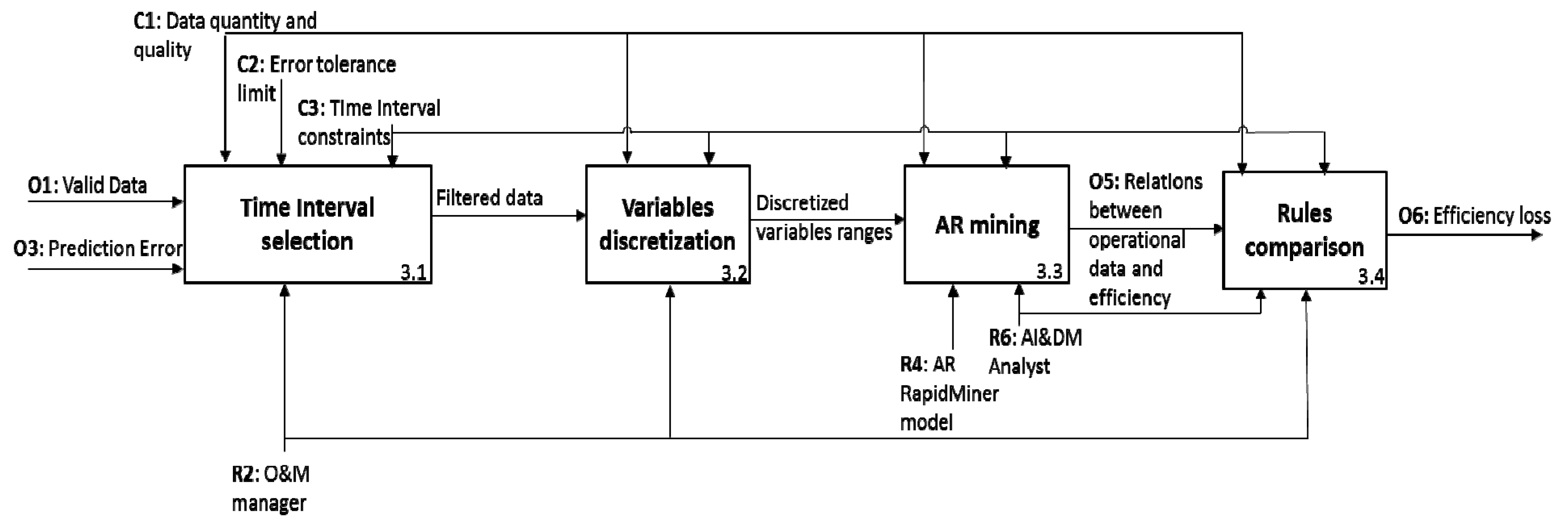
Time interval selection (IDEFØ 3.1): in order to check for any possible performance loss, we may want to compare situations belonging to different time intervals (C3), such as the efficiency before and after an overhaul or a failure of the equipment. For instance, we could select all the available data to develop as complete as possible analysis or select a symmetric time window, e.g., 1000 working hours before and after an overhaul.

(2)

In our application, according to the O&M manager (R2), we decided to consider the whole dataset, in order not to lose any information on the asset performance and to study only the filtered data relevant for the aim of the Data Mining step. Specifically, we split the dataset into 3 periods (

Table 7. Time intervals analyzed in our application.

Time Intervals	Number of Hours	Milestone
TI 1	3223	Overhaul
TI 2	4856	Failure
TI 3	49	Current date

): the first one, starts from the beginning of the system monitoring and lasts until the preventive Overhaul. The entire period would be composed of 13,772 working hours, but due to missing data and low quality ones, only 3223 can be considered in this study. The second time window, instead, ranges from the Overhaul to the catastrophic failure of the system (4856 of the 5173 working hours can be analyzed). After the failure of the asset, only 92 working hours are recorded, of whom 49 can be studied.

(3)

Variable selection and discretization (IDEFØ 3.2): depending on the depth of the analysis, we could filter some of the valid data determined in the first step, or limit the study to a certain number of variables. In addition, if the selected variables are measured through continuous values, a discretization is necessary since the AR mining algorithm applies to discrete elements. In our application, the variables selected are pressure, flow-rate, impulsion temperature, aspiration temperature, tank level, and density; all of them are related to the efficiency of the system.

(4)

The discretization process is performed in accordance with the O&M manager (R2). Indeed, a tradeoff is needed in this step: on the one hand, in fact, the discretization ranges have to be small enough to represent a specific operating condition. On the other hand, instead, we wish to have the greatest interval size, so that the system frequently operates inside it. In other words, if the intervals are too small, the system could work inside each of them very rarely and, consequently, we may not profit from the data. In the next table (

Table 8. List of variables, minimum values, maximum values and interval sizes.

Variable	Min Value	Max Value	Size
Flow rate [m3/h]	328	668	30
LNG Density [kg/m3]	430	465	5
Tank level [mm]	1900	35,900	1000
Intake Pressure [kg/cm2]	6.5	13.5	1
Intake Temperature [°C]	−160	−157	1
Impulsion Temperature [°C]	−160	−153	1
Efficiency [%]	42	68	1

) we report the minimum and maximum values of the valid data and the size chosen for each interval.

(5)

AR mining (IDEFØ 3.3): the discretized variables ranges represent the input of AR mining stage; quality of the results depends on data quality and availability (C1) and the temporal constraints considered (C3). The resources necessary to deploy the data mining procedure are O&M manager (R2) and the AI&DM analyst (R6), together with AR RapidMiner model (R4). According to the methodology explained in Section 3, we have to analyze the rules having values of the efficiency as head (Δ), and values of all the other selected variables as body (Γ). Each AR is associated with a support and a confidence: the former represents the percentage of time units over the total in which the operating conditions and the efficiency have assumed the values expressed by the rule. The latter, instead, indicates the probability of having the efficiency expressed by the rule, given the values of the operating variables. For example, in

Table 9. Example of the ARs extracted.

Flow Rate	Density	Tank Level	Pressure	T Asp	T Imp	Efficiency	Support	Confidence
[478–508]	[450–455]	[5900–6900]	[10.5–11.5]	[−159–−158]	[−158–−157]	[59–60]	0.0006	0.75
[478–508]	[450–455]	[5900–6900]	[10.5–11.5]	[−159–−158]	[−158–−157]	[59–60]	0.0002	0.25

, some of the rules extracted (O5) are reported. Column 1 to 6 (Flow rate, LNG Density, Tank level, Pressure, Intake Temperature, Impulsion Temperature) contain the body of the rule, while the seventh is the head (Efficiency); column 8 and 9, instead, respectively report the support and the confidence associated with each rule. The rules exemplified in Table 3, should be interpreted as follows (let’s consider, for instance, the first row): when the operating conditions of the system are characterized by a flow rate included in the range 478–508 m³/h, a density between 450 and 455 kg/m³, the tank level between 5900 and 6900 mm, the pressure inside the tank is between 10.5 and 11.5 kgf/cm³, the aspiration temperature (TAsp) is included in −159 °C and −158 °C and the impulsion temperature (TImp) is in −158 °C and −159 °C, in the 75% of the cases (confidence = 0.75), the efficiency of the system ranges between 59 and 60%; in the remaining 25% of the cases (see the second row of the table), instead, the efficiency range is 60–61%. The support associated with the former relation is 0.0006: this value indicates the probability of having the operating conditions values listed before and an efficiency level in 59–60%. Similarly, the rule associating the operating conditions values and the efficiency between 60–61% have a joint probability of occurrence, namely a support, of 0.0002.

(6)

Rules comparison (IDEFØ 3.4): The relations among the operating conditions and the efficiency (O5) mined in the previous step should be compared in order to verify the actual existence of an efficiency loss (O6) and the corresponding probabilities. To this end, we need to select rules presenting analogue values of the operating conditions but belonging to different time intervals, i.e., those identified in the first step of this stage. This activity has to be carried out both by the O&M manager (R2) and the DM&AI analyst (R6). In our study, three different time intervals have been selected and compared, as shown in Table 3. The highest number of comparable conditions characterizes TI 1 and TI 2: specifically, 58 common operating conditions have been identified in which the system under investigation works both before and after the overhaul (i.e., the milestone dividing TI 1 from TI 2). As shown in the following table (

Table 10. Efficiency comparison among the identified time intervals.

Time Intervals	Efficiency Comparison	Coincident Operating Conditions
TI 1 vs. TI 2	Efficiency TI 1 > Efficiency TI 2	54
	Efficiency TI 1 ≤ Efficiency TI 2	4
TI 1 vs. TI 3	Efficiency TI 1 ≤ Efficiency TI 3	16
TI 2 vs. TI 3	Efficiency TI 2 < Efficiency TI 3	3

), in almost the totality of the rules there is a loss of efficiency. Comparing the remaining time intervals, there are less coincident operating conditions. In general, the efficiency of the TI3 is higher than the one of TI 2 and greater-equal than the one of TI 1.

A more detailed example is reported in the following table (

Table 11. Rules comparison among the identified time intervals.

TI	Flow Rate	Density	Tank Level	Pressure	T Asp	T Imp	Efficiency	Support	Confidence
1	[508–538]	[445–450]	[27,900–28,900]	[11.5–12.5]	[−160–−159]	[−159–−158]	[64–65]	0.0003	0.5
	[508–538]	[445–450]	[27,900–28,900]	[11.5–12.5]	[−160–−159]	[−159–−158]	[65–66]	0.0003	0.5
2	[508–538]	[445–450]	[27,900–28,900]	[11.5–12.5]	[−160–−159]	[−159–−158]	[60–61]	0.0002	0.5
	[508–538]	[445–450]	[27,900–28,900]	[11.5–12.5]	[−160–−159]	[−159–−158]	[61–62]	0.0002	0.5
3	[508–538]	[445–450]	[27,900–28,900]	[11.5–12.5]	[−160–−159]	[−159–−158]	[64–65]	0.0204	0.5
	[508–538]	[445–450]	[27,900–28,900]	[11.5–12.5]	[−160–−159]	[−159–−158]	[65–66]	0.0204	0.5

). The first row contains the operating conditions and the corresponding efficiency in TI 1, while in the following three rows the analogue conditions and the efficiency values are reported for TI 2. In all cases, a decrease of the efficiency is noticed: indeed, in TI 1 its value is among 64% and 66%, while in TI2, efficiency values range among 60% and 62%. In TI 3, the efficiency increases, returning to the same range as TI 1. The interpretation of these results should be related to the preventive overhaul executed at the end of TI 1. Possibly, an error during the maintenance intervention or the re-installation occurred, compromising the performance of the entire asset and leading to a catastrophic failure at the end of TI 2. Indeed, in TI 3, the normal level of efficiency was reestablished.

As presented in this paragraph, the output of the output data analysis and control module are the relations among the operational, process, condition monitoring variables and efficiency and, after the comparison, a measure of the efficiency loss.

It is important to notice that modifying the head of the rule, i.e., replacing the efficiency with another attribute, allows moving the focus of the investigation. For example, it could be interesting to compare the operational variables with the failure modes, in order to associate different operating conditions with the most likely failure mode and prevent it through specific actions.

4.5. Decision Support Module

This last module of the IDEFØ 1 diagram is presented in Figure 9.

At this point of the process, the O&M manager can make decisions concerning possible changes in the normal operation and maintenance of the asset, but can also select a better strategy for the overhaul and reinvestment in the asset or its future replacement. These possibilities are constrained by the process flexibility sometimes, and may generate changes in equipment behavior that must be tracked and analyzed for possible re-training of the tool.

5. Implementation Process Results for the Pump Example

In our example, and concerning the scope of the project (as detailed in the introduction of Section 4), after a discussion with the General O&M Manager, the following was concluded:

• Concerning the prediction of anomalies in the operation of equipment with complex operation regime and poor monitoring of their condition through ANN AI-AR DM models:
  It was agreed that it is possible to model the behaviour of the pumps and detect anomalies in their operation by deviations from the prediction. For instance, it could be appreciated how a pump that suffered a catastrophic failure after its first overhaul, worked with anomalous behaviour throughout its second period of operation before the failure. Error accumulation was predicting this abnormal behaviour. Another clear appreciation was the punctual accumulations of error detected when the asset was reaching certain operating regimes.
• Concerning the guidelines for the practical implementation of the models in business systems:
  It was agreed that the systems are currently registering enough data to proceed with the implementation of this type of tools, and that it would be much more convenient to have all variables in a digital format and integrated the same information system, where the ANN algorithm is finally implemented. The implementation of the algorithm can be done by asset, for greater precision, without a significant increase in costs.
• Concerning the possibility to obtain information to build a business case:
  It was agreed that the integrated ANN-DM tool could avoid premature deterioration of equipment, verify the quality of its major maintenance intervention, ensure its operation at maximum energy efficiency, improve alarms and current interlocks for the operation of equipment, generate a new technical services to offer to potential clients, provide thoroughly understanding of the behaviour of pumps throughout their life cycle, adjust the periods of completion of major maintenance and estimate the health of the asset better (comparing with current available techniques).
• Concerning the identification and measurement of the asset´s loss of performance when anomalies are detected:
  It was agreed that the analysis of performance in similar operating regimes could be done properly. For instance, the measurement of the performance loss of the pump with the catastrophic failure, after its first overhaul could be done showing that the pump always operated with 4% to 6% lower performance. After the second overhaul, after the catastrophic failure, the pump recovered perfectly the initial performance.

In general terms, the implementation of the model has been considered a positive learning experience that can now be deployed for the entire fleet of similar assets, once the business case is approved. Another important aspect of this project implementation was to estimate the time schedule for this type of project. Figure 10 the percentage of time per process module accomplished when studying the first pump is presented. It is important to notice the following:

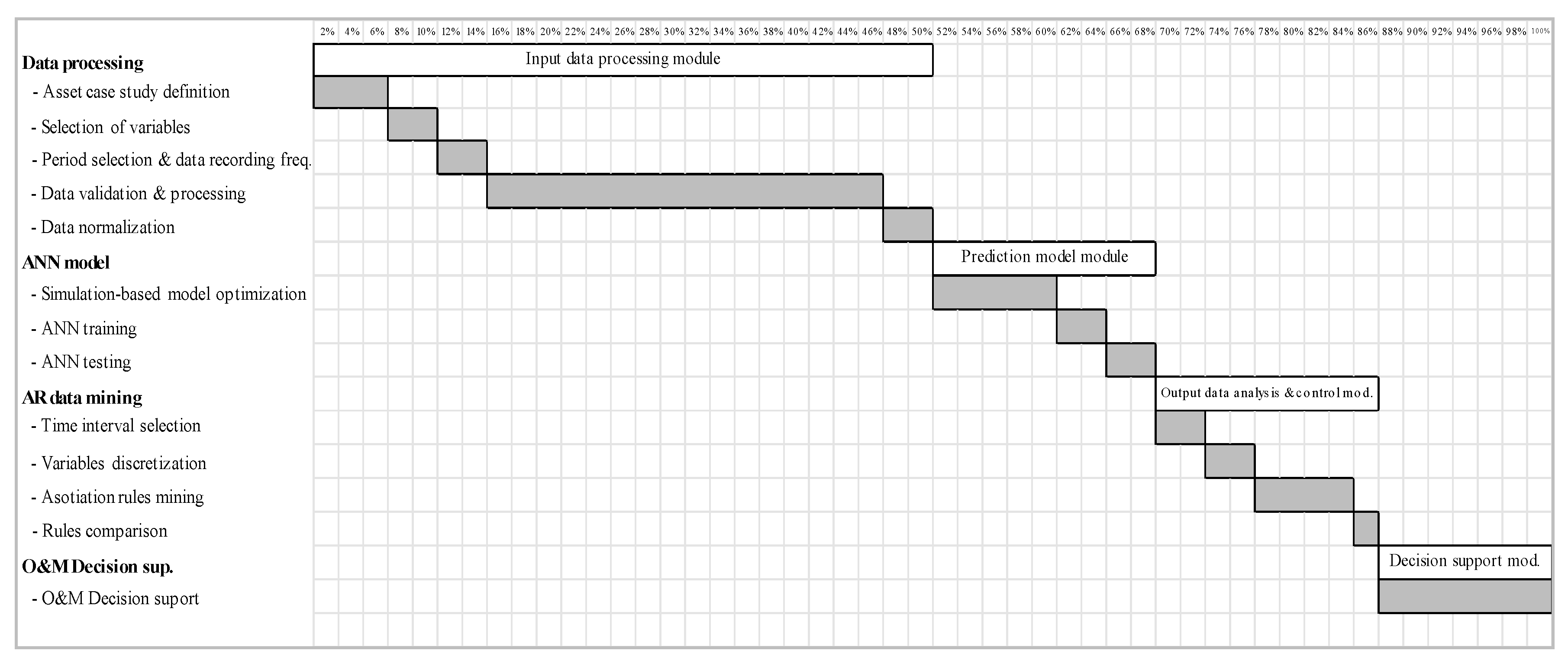
• The input data processing time resulted to be a 50% of the total project time in this initial implementation, as a result of the dispersion, different formats and quality of the data processed. The total time when replicating the study to a similar asset was reduced by 30%. Mainly impacting the input data processing module (20% time reduction), and the same impact in the next two modules (5% time reduction each).
• Time for data processing resulted longer than for prediction and data analysis modules together. This was shocking to the team involved in the project, even if the processing it is in line with the one indicated by the Cross Industry Standard Process for Data Mining (CRISP-DM), that consider it to be around the 70% of the total processing time [81]. The use of the AI-DM tools for the problem analysis was expected to be more time consuming than the data processing according to the complexity of the tools that were going to be used. However, two intermediate processes were really efficient and less dependent on circumstances out of the team control.

Being the current approach based on data, the main success factor of the methodology is data quality; however, this aspect can represent a major limitation for implementing it, since a substantial amount of data may not be immediately available in every company. At first, as noticed before, the procedure may appear time-consuming, but when it is included in the organizational routine, the obstacle characterized by the time for data validation and processing can be overcame. In addition, the application of ANN and AR mining requires an expertise in data understanding and modeling a positive mindset towards changing the current habits in terms of decision making in the O&M field.

6. Conclusions and New Research Opportunities

In this paper we deal with the problem of asset performance monitoring, to detect potential reliability problems and to predict loss of efficiency in energy consumption. We concentrated on assets with multiple operating conditions and low possibilities of components health monitoring.

This paper main contribution is a suggested method to tackle this problem, and the detailed explanation of the process accomplished, using the IDEFØ Functional Modeling method with three hierarchical series of diagrams, to implement the method in a complete case study. The resources and time needed for the project team to finalize the work were recorded.

The technical solution proposed considers the complementary application of the ANN (to detect when asset behavior abnormalities appear) and DM techniques (to detail the operating conditions for which behavior abnormalities were appreciated, and the extent of the impact on energy efficiency). The possibilities of the use of the AR mining tool, after the ANN, were tested and compared with alternative advanced method to ensure their suitability and accuracy.

Main limitations of the result proposed were found in the time needed for data processing. This activity was really time consuming for existing business conditions, due to data dispersion, different formats and quality of the data processed.

The overall case study project results showed that decision-making for the O&M manager could be improved by detecting any abnormal power consumption of the pump (through the accumulation of the square error of the prediction), with desired precision, and by releasing the corresponding process to measure the loss of energy efficiency when that happens. Additionally, it was proven how this process could serve to test the quality of major overhauls, to improve alarms and current interlocks and generally to provide a thorough understanding of the behavior of pumps throughout their entire life cycle.

Finally, it is important to mention that the idea is that the data processing for the ANN training would be done off-line, as well as the initial selection of variables intervals and rules for DM. Then, the information provided for O&M decision support could be generated on-line for the management.

References

- Borek, A.; Parlikad, A.K.; Woodall, P.; Tomasella, M. A risk based model for quantifying the impact of information quality. Comput. Ind. 2014, 65, 354–366. [Google Scholar] [CrossRef] [Green Version]
- Ouertani, Z.; Kumar, A.; McFarlane, D. Towards an Approach to Select an Asset Information Management Strategy. IJCSA 2008, 5, 25–44. [Google Scholar]
- Woodall, P.; Borek, A.; Parlikad, A.K. Data quality assessment: The Hybrid Approach. Inf. Manag. 2013, 50, 369–382. [Google Scholar] [CrossRef]
- Moore, W.J.; Starr, A.G. An intelligent maintenance system for continuous cost-based prioritisation of maintenance activities. Comput. Ind. 2006, 57, 595–606. [Google Scholar] [CrossRef] [Green Version]
- Kans, M.; Ingwald, A. Common database for cost-effective improvement of maintenance performance. Int. J. Prod. Econ. 2008, 113, 734–747. [Google Scholar] [CrossRef]
- Ashton, K. That ‘Internet of Things’ Thing. RFiD J. 2009, 22, 97–114. [Google Scholar]
- Atzori, L.; Iera, A.; Morabito, G. The Internet of Things: A survey. Comput. Netw. 2010, 54, 2787–2805. [Google Scholar] [CrossRef]
- Sarma, S.; Brock, D.; Ashton, K. The Networked Physical World; TR MIT-AUTOID-WH-001; MIT: Cambridge, MA, USA, 2000. [Google Scholar]
- Monostori, L.; Kádár, B.; Bauernhansl, T.; Kondoh, S.; Kumara, S.; Reinhart, G.; Sauer, O.; Schuh, G.; Sihn, W.; Ueda, K. Cyber-physical systems in manufacturing. CIRP Ann. 2016, 65, 621–641. [Google Scholar] [CrossRef]
- Davis, J.; Edgar, T.; Porter, J.; Bernaden, J.; Sarli, M. Smart manufacturing, manufacturing intelligence and demand-dynamic performance. Comput. Chem. Eng. 2012, 47, 145–156. [Google Scholar] [CrossRef]
- Lee, J.; Kao, H.A.; Yang, S. Service innovation and smart analytics for Industry 4.0 and big data environment. Procedia CIRP 2014, 16, 3–8. [Google Scholar] [CrossRef]
- Fayyad, U.M.; Irani, K.B. Multi-Interval Discretization of Continuous-Valued Attributes for Classification Learning. In Proceedings of the 13th International Joint Conference on Artificial Intelligence 1022–1027, Chambery, France, 28 August–3 September 1993. [Google Scholar]
- Diamantini, C.; Potena, D.; Storti, E. A virtual mart for knowledge discovery in databases. Inf. Syst. Front. 2013, 15, 447–463. [Google Scholar] [CrossRef]
- Shahbaz, M.; Srinivas, M.; Harding, J.A.; Turner, M. Product design and manufacturing process improvement using association rules. Proc. Inst. Mech. Eng. Part B J. Eng. Manuf. 2006, 220, 243–254. [Google Scholar] [CrossRef]
- Seng, N.Y.; Srinivasan, R. Data Mining for the Chemical Process Industry. In Encyclopedia of Data Warehousing and Mining, 2nd ed.; IGI Global: Hershey, PA, USA, 2009; pp. 458–464. [Google Scholar]
- Negri, E.; Fumagalli, L.; Macchi, M. A Review of the Roles of Digital Twin in CPS-Based Production Systems. Procedia Manuf. 2017, 11, 939–948. [Google Scholar] [CrossRef]
- European Committee for Standadization. EN13306: 2017, Maintenance Terminology; European Committee for Standadization: Brussels, Belgium, 2017. [Google Scholar]
- Niu, G.; Yang, B.S.; Pecht, M. Development of an optimized condition-based maintenance system by data fusion and reliability-centered maintenance. Reliab. Eng. Syst. Saf. 2010, 95, 786–796. [Google Scholar] [CrossRef]
- International Organization for Standardization. ISO 17359:2018—Condition Monitoring and Diagnostics of Machines—General Guidelines; International Organization for Standardization: Geneva, Switzerland, 2018. [Google Scholar]
- United States Army. ADS-79D-HDBK—Aeronautical Design Standard Handbook for Condition Based Maintenance Systems for US Army Aircraft; U.S. Army Aviation and Missile Research, Development and Engineering Center: Redstone Arsenal, AL, USA, 2013. [Google Scholar]
- Parra, C.; Crespo, A. Maintenance Engineering and Reliability for Assets Management; Ingeman: Seville, Spain, 2012. [Google Scholar]
- Jardine, A.; Lin, D.; Banjevic, D. A review on machinery diagnostics and prognostics implementing condition based maintenance. Mech. Syst. Signal Process. 2006, 20, 1483–1510. [Google Scholar] [CrossRef]
- Campos, J. Development in the application of ICT in condition monitoring and maintenance. Comput. Ind. 2009, 69, 1–20. [Google Scholar] [CrossRef]
- Lee, J.; Ghaffari, M.; Elmeligy, S. Self-maintenance and engineering immune systems: Towards smarter machines and manufacturing systems. Annu. Rev. Control 2011, 35, 111–122. [Google Scholar] [CrossRef]
- Vachtsevanos, G.; Lewis, F.; Roemer, M.; Hess, A.; Wu, B. Intelligent Fault Diagnosis and Prognosis for Engineering Systems; John Wiley and Sons: Hoboken, NJ, USA, 2006. [Google Scholar]
- Zio, E. Review reliabilty engineering: old problems and new challenges. Reliab. Eng. Syst. Saf. 2009, 94, 125–141. [Google Scholar] [CrossRef]
- Willis, H.L. Power Distribution Planning Reference Book; CRC Press: Boca Raton, FL, USA, 2004. [Google Scholar]
- González-Prida, V.; Guillén, A.; Gómez, J.; Crespo, A.; De la Fuente, A. An Approach to Quantify Value Provided by an Engineered Asset According to the ISO 5500x Series of Standards. In Asset Intelligence through Integration and Interoperability and Contemporary Vibration Engineering Technologies; Springer: Cham, Switzerland, 2019; pp. 189–196. [Google Scholar]
- Basheer, I.A.; Hajmeer, M. Artificial neural networks: Fundamentals, computing, design, and application. J. Microbiol. Methods 2000, 43, 3–31. [Google Scholar] [CrossRef]
- Zhang, G.; Patuwo, B.E.; Hu, M.Y. Forecasting with artificial neural networks: The state of the art. Int. J. Forecast. 1998, 14, 35–62. [Google Scholar] [CrossRef]
- Curry, B.; Morgan, P.; Beynon, M. Neural networks and flexible approximations. IMA J. Manag. Math. 2000, 11, 19–35. [Google Scholar] [CrossRef]
- Kuo, C. Cost efficiency estimations and the equity returns for the US public solar energy firms in 1990–2008. IMA J. Manag. Math. 2010, 22, 307–321. [Google Scholar] [CrossRef]
- Polo, F.A.O.; Bermejo, J.F.; Fernández, J.F.G.; Márquez, A.C. Failure mode prediction and energy forecasting of PV plants to assist dynamic maintenance tasks by ANN based models. Renew. Energy 2015, 81, 227–238. [Google Scholar] [CrossRef]
- Gibert, K.; Swayne, D.; Yang, W.; Voinov, A.; Rizzoli, A.; Filatova, T. Choosing the Right Data Mining Technique: Classification of Methods and Intelligent Recommendation. In Proceedings of the 5th Biennial Conference of the International Environmental Modelling and Software Society, iEMSs 2010, Ottawa, ON, Canada, 5–8 July 2010; pp. 2457–2464. [Google Scholar]
- Buddhakulsomsiri, J.; Siradeghyan, Y.; Zakarian, A.; Li, X. Association rule-generation algorithm for mining automotive warranty data. Int. J. Prod. Res. 2006, 44, 2749–2770. [Google Scholar] [CrossRef]
- Bermejo, J.F.; Fernández, J.F.G.; Polo, F.O.; Márquez, A.C. A Review of the Use of Artificial Neural Networks Models for Energy and Reliability Prediction. A Study for the Solar PV, Hydraulic and Wind Energy Sources. Appl. Sci. 2019, 9, 1844. [Google Scholar] [CrossRef]
- Bangalore, P.; Tjernberg, L.B. An artificial neural network approach for early fault detection of gearbox bearings. IEEE Trans. Smart Grid 2015, 6, 980–987. [Google Scholar] [CrossRef]
- Tehrani, M.M.; Beauregard, Y.; Rioux, M.; Kenne, J.P.; Ouellet, R. A predictive preference model for maintenance of a heating ventilating and air conditioning system. IFAC-PapersOnLine 2015, 28, 130–135. [Google Scholar] [CrossRef]
- Vernekar, K.; Kumar, H.; Gangadharan, K.V. Engine gearbox fault diagnosis using machine learning approach. J. Qual. Maint. Eng. 2018, 24, 345–357. [Google Scholar] [CrossRef]
- Martínez-Martínez, V.; Gomez-Gil, F.J.; Gomez-Gil, J.; Ruiz-Gonzalez, R. An Artificial Neural Network based expert system fitted with Genetic Algorithms for detecting the status of several rotary components in agro-industrial machines using a single vibration signal. Expert Syst. Appl. 2015, 42, 6433–6441. [Google Scholar] [CrossRef]
- Trappey, A.J.C.; Trappey, C.V.; Ma, L.; Chang, J.C.M. Intelligent engineering asset management system for power transformer maintenance decision supports under various operating conditions. Comput. Ind. Eng. 2015, 84, 3–11. [Google Scholar] [CrossRef]
- Prashanth, B.; Kumar, H.S.; Pai, P.S.; Muralidhara, R. Use of MEMS based vibration data for REB fault diagnosis. Int. J. Eng. Technol. 2018, 7, 714–718. [Google Scholar]
- Lazakis, I.; Raptodimos, Y.; Varelas, T. Predicting ship machinery system condition through analytical reliability tools and artificial neural networks. Ocean Eng. 2018, 152, 404–415. [Google Scholar] [CrossRef] [Green Version]
- Eyoh, J.; Kalawsky, R.S. Reduction of impacts of oil and gas operations through intelligent maintenance solution. In Proceedings of the International Conference on Intelligent Science and Technology-ICIST ’18, London, UK, 30 June–2 July 2018; pp. 67–71. [Google Scholar]
- De Benedetti, M.; Leonardi, F.; Messina, F.; Santoro, C.; Vasilakos, A. Anomaly detection and predictive maintenance for photovoltaic systems. Neurocomputing 2018, 310, 59–68. [Google Scholar] [CrossRef]
- Protalinsky, O.; Khanova, A.; Shcherbatov, I. Simulation of Power Assets Management Process; Springer: Cham, Switzarland, 2019; pp. 488–501. [Google Scholar]
- Agrawal, R.; Imieliński, T.; Swami, A. Mining association rules between sets of items in large databases. ACM SIGMOD Rec. 1993, 22, 207–216. [Google Scholar] [CrossRef]
- Chen, W.C.; Tseng, S.S.; Wang, C.Y. A novel manufacturing defect detection method using association rule mining techniques. Expert Syst. Appl. 2005, 29, 807–815. [Google Scholar] [CrossRef]
- Kamsu-Foguem, B.; Rigal, F.; Mauget, F. Mining association rules for the quality improvement of the production process. Expert Syst. Appl. 2013, 40, 1034–1045. [Google Scholar] [CrossRef] [Green Version]
- Martínez-De-Pisón, F.J.; Sanz, A.; Martínez-De-Pisón, E.; Jiménez, E.; Conti, D. Mining association rules from time series to explain failures in a hot-dip galvanizing steel line. Comput. Ind. Eng. 2012, 63, 22–36. [Google Scholar] [CrossRef]
- Sammouri, W.; Come, E.; Oukhellou, L.; Aknin, P.; Fonlladosa, C.-E. Floating train data systems for preventive maintenance: A data mining approach. In Proceedings of the 2013 International Conference on Industrial Engineering and Systems Management (IESM), Rabat, Morocco, 28–30 October 2013; pp. 1–7. [Google Scholar]
- Bastos, P.; Lopes, I.D.; Pires, L. A maintenance prediction system using data mining techniques. World Congr. Eng. 2012, 3, 1448–1453. [Google Scholar]
- Djatna, T.; Alitu, I.M. An Application of Association Rule Mining in Total Productive Maintenance Strategy: An Analysis and Modelling in Wooden Door Manufacturing Industry. Procedia Manuf. 2015, 4, 336–343. [Google Scholar] [CrossRef] [Green Version]
- Antomarioni, S.; Bevilacqua, M.; Potena, D.; Diamantini, C. Defining a data-driven maintenance policy: An application to an oil refinery plant. Int. J. Qual. Reliab. Manag. 2019, 36, 77–97. [Google Scholar] [CrossRef]
- Antomarioni, S.; Pisacane, O.; Potena, D.; Bevilacqua, M.; Ciarapica, F.E.; Diamantini, C. A predictive association rule-based maintenance policy to minimize the probability of breakages: Application to an oil refinery. Int. J. Adv. Manuf. Technol. 2019. [Google Scholar] [CrossRef]
- Nisi, M.; Renga, D.; Apiletti, D.; Giordano, D.; Huang, T.; Zhang, Y.; Mellia, M.; Baralis, E. Transparently Mining Data from a Medium-Voltage Distribution Network: A Prognostic-Diagnostic Analysis. In Proceedings of the EDBT/ICDT 2019 Joint Conference, Lisbon, Portugal, 26–29 March 2019. [Google Scholar]
- Hu, L.; Liu, K.-Y.; Diao, Y.; Meng, X.; Sheng, W. Operational Reliability Evaluation Method Based on Big Data Technology. In Proceedings of the 2016 International Conference on Cyber-Enabled Distributed Computing and Knowledge Discovery (CyberC), Chengdu, China, 13–15 October 2016; pp. 341–344. [Google Scholar]
- Lawrence, S.; Giles, C.; Tsoi, A. What Size Neural Network Gives Optimal Generalization? Convergence Properties of Backpropagation; University of Maryland Libraries: College Park, MD, USA, 1996. [Google Scholar]
- Ali, S.; Smith, K.A. On learning algorithm selection for classification. Appl. Soft Comput. J. 2006, 6, 119–138. [Google Scholar] [CrossRef]
- Bengio, Y.; Simard, P.; Frasconi, P. Learning Long-Term Dependencies with Gradient Descent is Difficult. IEEE Trans. Neural Netw. 1994, 5, 157–166. [Google Scholar] [CrossRef] [PubMed]
- Lapedes, A.; Farber, R. Nonlinear Signal Processing Using Neural Networks: Prediction and System Modeling. In IEEE-Neural Networks; National Technical Information Service, U.S. Department of Commerce: Springfield, VA, USA, 1987. [Google Scholar]
- Han, J.; Cheng, H.; Xin, D.; Yan, X. Frequent pattern mining: current status and future directions. In Data Mining and Knowledge Discovery; Springer Science + Business Media: Berlin, Germany, 2007; pp. 55–86. [Google Scholar]
- Mata, J.; Alvarez, J.L.; Riquelme, J.C. An evolutionary algorithm to discover numeric association rules. In Proceedings of the 2002 ACM Symposium on Applied Computing, Madrid, Spain, 11–14 March 2003. [Google Scholar]
- Mirebrahim, S.H.; Shokoohi-Yekta, M.; Kurup, U.; Welfonder, T.; Shah, M. A Clustering-based Rule-mining Approach for Monitoring Long-term Energy Use and Understanding System Behavior. In Proceedings of the 4th ACM International Conference on Systems for Energy-Efficient Built Environments, Delft, The Netherlands, 8–9 November 2017; pp. 5:1–5:9. [Google Scholar]
- Jović, A.; Brkić, K.; Bogunović, N. An overview of free software tools for general data mining. In Proceedings of the 2014 37th International Convention on Information and Communication Technology, Electronics and Microelectronics, MIPRO 2014-Proceedings, Opatija, Croatia, 26–30 May 2014. [Google Scholar]
- Announcing the Standard for Integration Definition for Function Modeling (IDEF0); U.S. Department of Commerce: Springfield, VA, USA, 1993.
- Theodoridis, S. Probability and Stochastic Processes. In Probability and Stochastic Processes, Machine Learning; Academic Press: Cambridge, MA, USA, 2015; pp. 9–51, Chapter 2. [Google Scholar]
- Powell, M.J.D. An efficient method for finding the minimum of a function of several variables without calculating derivatives. Comput. J. 1964, 7, 155–162. [Google Scholar] [CrossRef]
- Powell, M.J.D. On the calculation of orthogonal vectors. Comput. J. 1968, 11, 302–304. [Google Scholar] [CrossRef] [Green Version]
- Li, Z.; Rahman, S.M.; Vega, R.; Dong, B. A hierarchical approach using machine learning methods in solar photovoltaic energy production forecasting. Energies 2016, 9, 55. [Google Scholar] [CrossRef]
- Boser, B.E.; Guyon, I.; Vapnik, V. A training algorithm for optimal margin classifiers. In Proceedings of the Fifth Annual Workshop on Computational Learning Theory, Pittsburgh, PA, USA, 27–29 July 1992; pp. 144–152. [Google Scholar]
- Chen, J.L.; Liu, H.B.; Wu, W.; Xie, D.T. Estimation of monthly solar radiation from measured temperatures using support vector machines—A case study. Renew. Energy 2011, 36, 413–420. [Google Scholar] [CrossRef]
- Zhang, H.; Chen, L.; Qu, Y.; Zhao, G.; Guo, Z. Support vector regression based on grid-search method for short-term wind power forecasting. J. Appl. Math. 2014, 2014, 835791. [Google Scholar] [CrossRef]
- Meyer, D.; Dimitriadou, E.; Hornik, K.; Weingessel, A.; Leisch, F. e1071: Misc Functions of the Department of Statistics, Probability Theory Group (Formerly: E1071); R Package Version 1.6-7; TU Wien: Vienna, Austria, 2015. [Google Scholar]
- Fan, R.E.; Chang, D.K.-W.; Hsieh, C.-J.; Wang, X.-R.; Lin, C.-J. LIBLINEAR: Una biblioteca para la Clasificación grande lineal. J. Mach. Learn Investig. 2008, 9, 1871–1874. [Google Scholar]
- Helleputte, T. LIBLINEAR: Modelos lineales predictivos basados en la LIBLINEAR C/C++ R library versión. 2015. [Google Scholar]
- Elyan, E.; Gaber, M.M. A genetic algorithm approach to optimising random forests applied to class engineered data. Inf. Sci. 2017, 384, 220–234. [Google Scholar] [CrossRef]
- Lin, Y.; Kruger, U.; Zhang, J.; Wang, Q.; Lamont, L.; Chaar, L.E. Seasonal analysis and prediction of wind energy using random forests and ARX model structures. IEEE Trans. Control Syst. Technol. 2015, 23, 1994–2002. [Google Scholar] [CrossRef]
- Moutis, P.; Skarvelis-Kazakos, S.; Brucoli, M. Decision tree aided planning and energy balancing of planned community microgrids. Appl. Energy 2016, 161, 197–205. [Google Scholar] [CrossRef] [Green Version]
- Liaw, A.; Wiener, M. Classification and regression by RandomForest. R News 2002, 2, 18–22. [Google Scholar]
- Chapman, P.; Clinton, J.; Kerber, R.; Khabaza, T.; Reinartz, T.; Shearer, C.; Wirth, R. The CRISP-DM user guide. In Proceedings of the 4th CRISP-DM SIG Workshop in Brussels in March (1999), Brussels, Belgium, 18 March 1999. [Google Scholar]