Abstract
Strong coupling in an inductive power transfer (IPT) system will lead to difficulties in power control and loss of soft switching conditions. This paper presents an IPT system that can decouple the converter from the resonant network. In the proposed system, the energy transmission process is divided into energy injection stage and free resonance stage. In the energy injection stage, the inductor is separated from the resonance network, and the power source injects energy into the inductor independently. In the free resonance stage, the inductor is connected to the resonance network for resonating. As a benefit from the decoupling of the converter from the resonance network, the proposed IPT system is characterized by easy power control and soft switching operation. A prototype was built for experiments. The experimental results show that with a supply voltage of 300 V, coupling factor of 0.2, and load resistance of 10 Ω, the output power can be controlled nearly linearly by the time of the energy injection stage in a range of 40–60 μs, and the system works under soft switching conditions.
1. Introduction
The inductive power transfer (IPT) system is a method of delivering power from a source to a load wirelessly, with the advantages of flexibility, safety, and convenience. IPT system has been widely used in wireless power transfer (WPT) systems, such as mobile phones [1], medical transplants [2], and electric vehicle (EV) charging applications [3,4,5,6,7]. IPT system has a pair of coils, which can be regarded as a loosely coupled transformer [8,9]. However, in a loosely coupled transformer, the leakage inductance is large and the coupling between the primary and secondary side is weak, resulting in low efficiency and power. To solve this problem, the resonant networks are employed on the primary and secondary side to compensate the reactive power caused by the leakage inductance [10]. Previous literature has studied the compensation methods. These methods include the basic topologies of S/S, S/P, P/S, and P/P [11,12], together with the hybrid compensation topologies, such as LCL [3,13] and LLC [14]. These works partly solved the low power and low efficiency caused by the leakage of the loosely coupling transformer, and made the IPT system work well under stable conditions.
However, the resonant frequency is significantly varied as the magnetic coupling between the primary coil and secondary coil changes due to the air-gap variation, lateral misalignment, and longitudinal movement [15]. These variations will lead to changes in coefficients of the loosely coupling transformer and frequency drift, resulting in frequency detuning and decreases in efficiency and power [15,16,17,18]. Some methods using phase-locked loop (PLL) are employed for frequency tracking. Matysik [19] introduces a frequency tracking method by adjusting the phase shift of current and voltage in resonant tank. Gati et al. [20] employs a digital PLL to zero the phase shift of the secondary current and the voltage of inverter. Using this method, the system can track the frequency well. However, to ensure the soft switching conditions, switching should occur at zero (near-zero) current. Therefore, an integrated control method [21] should be used to control the switches of the converter.
In the IPT systems, input voltage or load often changes, and it is necessary to change the power delivered to the primary side or secondary side. Therefore, power flow control plays an important role in the optimization of the IPT system’s operation [22]. Traditional power control methods include reactive power control [23], frequency control [24] and phase shifting [25]. However, these power control methods still have problems such as the switching losses and electromagnetic noise, due to the operating devices are not always under soft switching conditions [26,27].
By dividing the energy transmission process into an energy injection stage and a self-tuning resonance stage (the converter maintain resonance by self-oscillation), the power can be controlled by the cycle number of the self-tuning resonance [28,29]. In these methods, all switching of the devices operate at the zero-crossing point of the primary current. Similar to the phase-locked loop control method, this power control method also needs switching operation at zero-crossing point of primary current. Therefore, the integrated control method should be used too for soft switching operation.
As mentioned in [21], to implement the integrated control methods, the supported hardware and control algorithm are needed. The hardware usually includes special signal unit, dead time pulse unit, phase-locked generator, and some logic devices. That is to say, a complex control circuit and control process are needed.
The complex control of the IPT system is due to the strong coupling between the resonant network and the converter. The operation of the converter is required to match the resonant network. If the converter can be decoupled from the resonant network during the energy injection period, the operation of the converter will not be restricted by the resonant network. Without the restriction of resonant network, the converter switches may be easily operated under soft switching condition, and the power flow may be easily controlled [30].
This paper presents a converter for IPT system based on independently inductive energy injection and free resonance (IIEIFR) control strategy. In contrast to traditional converters, the proposed converter has independent energy injection topology and free oscillation topology. The control strategy is different from the traditional converters either. With the proposed control strategy, the resonant tank is completely isolated from the power supply in the energy injection stage, and the power source injects energy into the inductor independently.
The proposed converter has two operating states: energy injection state and free resonance state. In the energy injection state, the primary inductor is isolated from the resonance network and connected to the power source. The power source independently injects energy into the primary inductor. In the free resonance state, the primary inductor is isolated from the power source and connected back to the resonance network, and the system begins to resonate freely. Two semiconductor devices are used as two double-throw switches to switch the system between the two states. Since the energy injection state and the resonance state are isolated from each other, the converter can be decoupled from the resonance network by using IIEIFR control strategy. This IPT system has the following characteristics:
- (1)
- Energy injection process is not affected by the resonance network. Therefore, the power flow can be independently controlled by changing the period of the energy injection stage.
- (2)
- There is no energy backflow in the free resonance state, and the reactive power can be eliminated.
- (3)
- Two time margins of the state transition are applied in the proposed control strategy. Therefore, there are soft switching time periods in the switching operation and the switches need not to be switched at zero current crossing point.
2. Basic Structure and System Models
2.1. Structure of the IIEIFR IPT System
A sketch of the IIEIFR IPT system is shown in Figure 1. It consists of a power source UDC, a primary tank capacitor Cp, a primary inductor L1, a secondary tank capacitor Cs, a secondary inductor L2, a double-throw switches K and a load resistance R. M is the mutual inductance between L1 and L2. L1, L2, and M can be described as a loosely coupled transformer T.
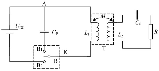
Figure 1.
The conceptual schematic of the IIEIFR system.
The fixed end of switch K is identified as B, and the switchable ends of K are identified as B1 and B2, respectively. According to the connection states of K, the IIEIFR IPT system can work in three stages:
- (1)
- Energy injection stage. In this stage, B is connected to B2. UDC is connected to L1 and L1 is isolated from Cp. UDC independently injects energy into the primary coil. In this stage, part of the energy is transferred to the secondary coil, as shown in Figure 2a. In Figure 2, the activated circuit parts were indicated by solid lines and inactive circuit parts were indicated by dashed lines.
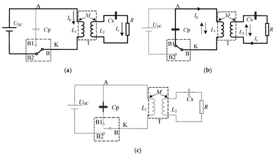 Figure 2. Schematic diagram of IIEIFR system. (a) Energy injection stage; (b) Free resonance stage; (c) Shutdown stage.
 - (2)
- Free resonance stage. In this stage, B is connected to B1. UDC is isolated from L1, and Cp is connected to L1 to form a resonant tank and the system begins to resonate, as shown in Figure 2b. The energy continues to be transferred to the secondary coil.
- (3)
- Shutdown stage. B is switched to the center point, not connected to either B1 or B2, where UDC, Cp, and L1 are isolated from each other, as shown in Figure 2c. In this stage, the system stops transferring energy to the secondary part and the remaining energy is stored in the capacitor Cp as electrical energy.
2.2. System Modeling
2.2.1. Energy Injection Stage
In this stage, the primary inductor is connected to the power source, and Figure 1 can be simplified to Figure 3a. In Figure 3a, N1 and N2 are the turns of the primary and secondary coils, respectively (in this study, N1 = N2). With the coupled inductors model (M model), Figure 3a can be represented by Figure 3b.
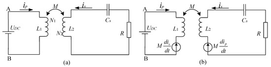
Figure 3.
Circuit models in the energy injection stage (a) simplified circuit model; (b) equivalent circuit model.
In Figure 3b, ip is the primary current; is is the secondary current. Coupling capacity between primary and secondary can be expressed by coupling coefficient k, then there is:
2.2.2. Free Resonance Stage
In the free resonance stage, the primary inductor L1 is connected with the capacitor Cp to form a resonance tank, and Figure 1 can be illustrated as Figure 4a. Since the currents in the primary inductor and secondary inductor are sinusoidal, Figure 4a can be simplified to Figure 4b.
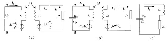
Figure 4.
Circuit models in the free resonance state stage: (a) simplified circuit model; (b) equivalent circuit model under sinusoidal condition; (c) equivalent circuit of the primary.
According to the method provided in the literature [12,31], secondary impedance can be expressed as
The loading effect of the secondary side on the primary side can be shown as a reflected impedance, as shown in Figure 4c. there is
Assuming , the frequency of the system in the free resonance mode is
In this case, the reactance of Zs is zero, and the reflected impedance is reduced to a resistance RC = Re{Zr}.
3. IIEIFR Power Converter
3.1. Topology of the IIEIFR IPT System
The system configuration of an IIEIFR IPT system is shown in Figure 5. In Figure 5, S1 and S2 are employed to perform the function of the double-throw switch as shown in Figure 1. D3 is anti-backflow diode. T is the loosely coupled transformer used for energy transmission with primary and secondary coils. L1 is the inductance of primary coil and L2 is the inductance of secondary coil, k is the coupling coefficient. Cp is the primary resonant capacitor and Cs is the secondary resonant capacitor. One terminal of the primary coil is connected to the positive electrode of the power source, and the other terminal is connected to point B between S1 and S2. When S1 is turned on and S2 turned off, point B is connected to Cp, and the system is in the free resonance stage. When S1 is turned off and S2 is tuned on, point B is connected to the negative electrode of the power source, and the system is in the energy injection stage. To prevent Cp directly connecting to the power source to generate surge current, a control strategy is used to ensure that S1 and S2 do not be turned on simultaneously.
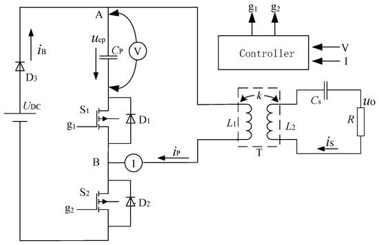
Figure 5.
The structure of IIEIFR converter.
A voltage sensor is used to detect the voltage across the Cp and a current sensor is used to detect the primary current flowing through L1, and a controller is employed to control the operation of the system. Signals of the sensors are sent to the controller, and the control strategy of the controller generates control signals, g1, g2, to control S1 and S2, respectively.
3.2. State Analysis
Figure 6 shows the state transition process of an IIEIFR converter. The steps of the state transition are indicated by schematic diagrams, and each step is indicated by a consecutive number from ① to ⑤. The energy transmission process of the IIEIFR converter can be divided into 3 main states and 2 transitional states. The main states are energy injection state (state ①); free resonance state (state ③), and shutdown stage (state ⑤). The transition states are transition state between the energy state and the free resonance state (state ②); transition state between the free resonance state and shutdown state (state ④). Big arrows are used to indicate the order of state transitions. The current-carrying devices and circuit parts are indicated by black solid line, and the voltage-blocking devices and circuit parts are indicated by dashed lines.
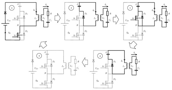
Figure 6.
State transitions of the IIEIFR converter.
The waveforms of ucp, ip and iB of the IIEIFR converter in an energy transmission period is illustrated in Figure 7. Each state is also represented by a consecutive number in Figure 7, which is consistent with those in Figure 6.
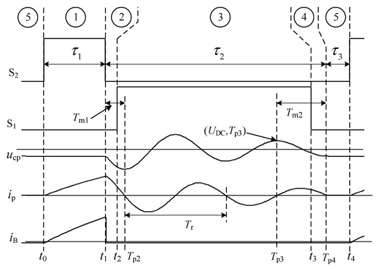
Figure 7.
The waveforms of the bus current, primary current, and tank capacitor voltage of the IIEIFR converter.
As shown in Figure 6 and Figure 7, the working principle and states of the IIEIFR converter are analyzed as follows:
State ⑤ [t < t0]: Shutdown state of the former energy transfer period. In this state, S1 and S2 are all turned off, the current of L1 is zero, and the voltage across Cp is −UDC. The energy remaining in the former period is stored in the Cp.
State ① [t0,t1]: This state is the energy injection state, indicated as the energy injection period of τ1 in Figure 7. In this state, S1 is turned off and S2 is turned on, the point B is connected to negative electrode of the power source UDC, and the primary inductor is connected to UDC. The source current iB and the primary inductor current ip, (iB = ip) flow through S2, increasing linearly from zero, and UDC injects energy into the primary inductor L1. As S1 is turned off, Cp is separated from point B, Cp and L1 are isolated from each other, and ucp is maintained at −UDC. In this way, the power source is decoupled from the resonant tank.
According to Figure 3b, the voltage and current equation of state ① are:
As shown in Figure 7, at time t0, there is ip(t0) = 0. For convenience of analysis, let t0 = 0. From Figure 3b and Equation (1), and assume L = L1 = L2, it can be got that:
Using Equation (6) as the boundary condition, solve Equation (5) and get
where
IPT system generally works in low coupling coefficient condition (k < 0.3) [32], therefore, the first term of the Equation (7) can be ignored, and the Equation (7) can be simplified as
Equation (9) indicates that the IIEIFR converter input current increases linearly and is not affected by other factors during the energy injection state. This characteristic enables the IIEIFR IPT system to conveniently control output power.
At t1, ip reaches the maximum as ip (t1). Define as the energy injection period, there is
In the energy injection period, the magnetic energy injected into the primary inductor by the power source is
As can be seen in Figure 7, before t1, the voltage of ucp is maintained at −UDC, which indicates that the Cp stores the remained energy in the previous energy transmission period.
When the system is switched from the energy injection state to the free resonance state, this residual energy needs to be added to the resonance network. Therefore, a transition state is required to do this.
State ② [t1, t2]: This state is the transitional state between the energy injection state and the free resonance state. In this state, S2 is turned off, and D1 is turned on. The current ip does not flow through S2 but through D1 to charge the capacitance Cp, and iB is interrupted. With charging to Cp by ip, ucp decreases from −UDC and ip decreases from the maximum current ip (τ1). By this way, the energy stored in Cp is added to the resonance network. Since at this time the circuit was in resonance, both ip and ucp drop sinusoidally. At Tp2, ucp drops to the lowest point while ip drops to zero.
Note in the interval [t1, Tp2], D1 maintains in on state, and the voltage across S2 is zero, which creates zero voltage switch (ZVS) condition of turning on S2. Therefore, the interval [t1, Tp2] can be defined as a time margin, Tm1 for turning on S2 under ZVS condition when the system transitions from state ① to state ②. During Tm1, a certain t2 is chosen to turn on S1, and the system is switched to the free resonance state.
State ③ [t2, t3]: This state is the free resonance state. Since both S1 and D1 are alternately turned on in this state, point B is connected to the capacitor Cp, and L1 and Cp form a resonant tank. As the system begins to resonant, the energy is transferred to the secondary side, and the amplitudes of the ucp and ip decrease exponentially.
When the amplitude of ucp drops to UDC, (at Tp3, as shown in Figure 7), most of the injected energy has been sent to the secondary side. Therefore, when the voltage sensor (as shown in Figure 5) detects ucp = UDC, the controller executes a program to make the system exit from the free resonance state. A transition state is needed to convert magnetic energy into electric energy before exiting the free resonance state.
State ④ [t3, t4]: This state is the transitional state between the free resonance state and shutdown state. As shown in Figure 7, at time moment Tp3, the amplitude of ucp drops to UDC, and correspondingly ip is zero. After Tp3 moment, ip flows forward to charge Cp through D1. With the charging of Cp, the magnetic energy is converted into electrical energy. At time moment Tp4, ip drops to zero again and ucp reaches to −UDC. This means that all magnetic energy has been converted into electric energy. If an appropriate t3 is chosen to turn off S1 in the interval [Tp3, Tp4], the backflow path of ip will be blocked. Therefore, ip will be zero after Tp4, and ucp will remain at −UDC until the next energy transfer period.
In this state, as the switch control strategy is based on voltage and current sensors, the condition to turn off S1 is that ip must be positive and in the time interval [t3, t4]. If ip is not positive due to load change, S1 will not be turned off because it does not meet the turn-off condition. The turn-off action will be postponed to the next cycle (after the system is stable).
In the interval [Tp3, Tp4], D1 is in on state, which creates ZVS condition of turning off S1. Therefore, the interval [Tp3, Tp4] can be defined as the time margin Tm2, for turning off S1 when system is to exit the free resonance state.
In fact, the system is in the same resonance period in states ②, ③, ④, and the interval [t1, Tp4] can be defined as a free resonance period τ2, as shown in Figure 7. In the interval [t1, Tp4], Figure 5 is equivalent to the circuit shown in Figure 4b, and the voltage equation is shown as
According to [27,33], the solution of Equation (12) is
where
Equation (13) has two unknown valuables to be solved, i.e., the amplitude Ipm, and phase lead angle θ. In Figure 7, it can be seen that at the moment t1, ip is the maximum ip (t1), and ucp (t1) is −UDC. According to Figure 4b, there is
Let t1 = 0, there are: ip (0) = ip (t1) = ip (τ1), ucp (0) = ucp (t1) = −UDC. Substituting these initial conditions into Equation (13), there are
The amplitude Ipm and phase angle θ in Equation (13) can be obtained by solving Equation (16). There are
State ⑤: The shutdown state. After Tp4, both S1 and S2 are turned off. The primary current ip = 0 and the capacitor voltage ucp = −UDC. The circuit stopped transferring the energy temporarily and waited for the next energy transmission process.
3.3. Parameter Settings
3.3.1. Time Parameters
Time margins for state change (Tm1 = Tp2 − t1, Tm2 = Tp4 − Tp3). As shown in Figure 7, Tm1 is the time of the lead angle of ip, and Tm2 is the time of half a cycle of ip. Therefore, Tm1 and Tm2 can be calculated by
Maintenance time of free resonance state. Due to the low coupling coefficient, the energy injected into the resonant tank needs multiple cycles to be sent to the secondary side in τ2. As shown in Figure 7, two cycles are used to transfer energy to the secondary side in one energy transfer process. According to the different coupling coefficients, the cycle numbers in τ2, n, are different in an energy transmission process. Therefore, τ2 is a function of the coupling coefficient k.
As can be seen from ip curve in Figure 7, τ2 contains two resonant cycles and one Tm1, therefore, for the general case, τ2 can be expressed as
where n is the numbers of the free resonance cycle, and Tr is the period of the free resonance. The theoretical n and Tr has been studied in [30] as
where [·] is the integer function. Please note that the number of the resonance cycles must be an integer.
3.3.2. Output Power
Since the switches of the converter operate under soft switching condition, the loss level of the converter is low. The energy injected in energy injection state can be considered to be all sent to the secondary coil. As shown in Figure 7, the time required for an energy transmission period is
According to Equations (11) and (21), the output power is
4. Experimental Prototype
To demonstrate the proposed topology of the IIEIFR IPT system, according to the topological structure of Figure 5, an experimental prototype was built. The prototype has a power capacity of 1000 W and consists of two parts: the power converter and the magneto-electric system.
4.1. Magneto-Electric System
The magneto-electric system is a pair of coil pad, and the pad structure is shown in Figure 8. An epoxy resin plate is placed on the bottom layer as a substrate. Several pieces of ferrites (Mn–Zn ferrite PC40) are radially placed on the substrate to form a core layer. A copper coil is wound by Litz wires (diameter 500 × 0.1 mm) on the core layer. Upon the copper coil is a protective layer made of organic glass. The structure of the primary pad is the same as the secondary pad, and its geometric dimensions are listed in Table 1.
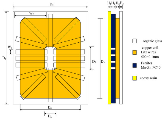
Figure 8.
Structure of the pad used.

Table 1.
Geometrical dimensions of the pads.
The inductances of the coil pads are both 640 μH, and the mutual inductance between the pads varies with the air gap of the pads. The coupling coefficient versus air gap is shown in Figure 9, when the gap increases from 50 mm to 210 mm, the coupling coefficient decreases from 0.51 to 0.06 respectively, matching the range of EV charging system, 0.1–0.33 [32].
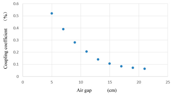
Figure 9.
Coupling coefficient versus the air gap.
4.2. Power Converter
The prototype of the power converter that was built according the topology illustrated in Figure 5 is shown in Figure 10. The prototype parameters are shown in Table 2, and the controller of the prototype is the microprocessor STM32.
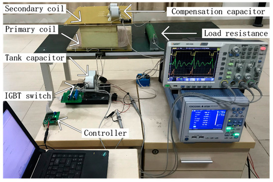
Figure 10.
The prototype of the IIEIFR IPT system.
Table 2.
Component values used in the prototype.
5. Simulation and Experimental Verification
5.1. Features of the IIEIFR ICP System
In the processes of simulation and experiment, τ1 = 70 μs, τ3 = 50 μs, k = 0.2, UDC = 300 V and R = 10 Ω. ug1 and ug2 are control signal of S1 and S2, respectively. ucp is the voltage of capacitor Cp. ip is the current of L1. iB is the current of power source. The simulation results using SABER (Synopsys, Mountain View, CA, USA) are shown in Figure 11. The experimental results are shown in Figure 12. These results are consistent with the descriptions in Figure 7 and Section 3.2.
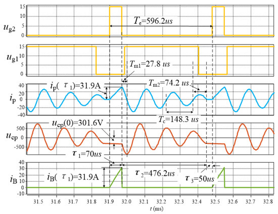
Figure 11.
The simulation result of the IIEIFR ICPT system.
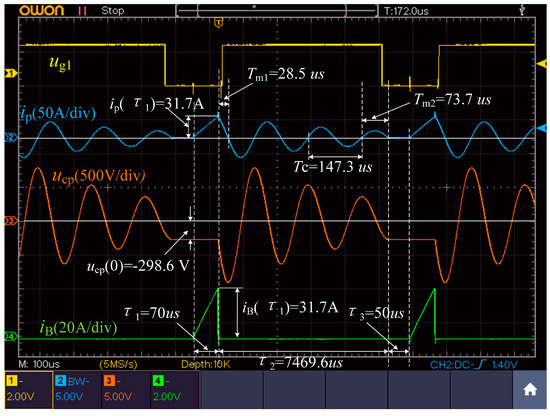
Figure 12.
The experiment result of the IIEIFR ICP system.
τ1 is the energy injection maintenance time, in this period, iB and ip rise linearly from zero. This indicates that the power source independently injects energy into the inductor L1. At the end of τ1, iB and ip rise to the maximum, iB(τ1) and ip(τ1). During this period, ucp is at its initial value, ucp = ucp (0), and remains unchanged because Cp is isolated from L1. τ2 is the free resonance maintenance time. In this period, ip and ucp change sinusoidally, and iB remains zero. This indicates that Cp and L1 form a resonant tank and begin to resonate, and the power source is isolated from L1, stopping the energy injection. Since energy is sent to the secondary side, the amplitudes of ip and ucp decrease exponentially during free resonance. At the end of τ2, ucp returns to the initial value, ucp = ucp (0) again, and ip drops to zero, the free resonance stops. Simulation and experimental results show that energy injection and free resonance are independent of each other, which proves that the converter of the IIEIFR system is decoupled from the resonant network and there is no energy backflow.
According to Table 2, some parameters of this prototype were calculated by Equations (10)–(20) and listed in Table 3. Comparing Figure 11 with Table 3, it can be seen that the simulation and the experimental results are consistent with the theoretical calculation.
Tm1 is the time margin for switching from the energy injection state to the free resonance state, it can be seen that ug1 rises in this time margin to turn on S1. Tm2 is the time margin for switching from the free resonance state to the shutdown state, it can be seen that ug1 drops in this time margin to turn off S1.
The period of ug2 is the period of energy injection period, and the period of ug2 is Te = τ1 + τ2 + τ3. Tc is the cycle of the free resonance, and there are three cycles of ip in a period of ug2, which means the IIEIFR converter can carry out high frequency energy transmission at low switching frequency, and this feature reduces the switching losses.
Figure 13 shows the waveforms of primary current, the secondary current (output current) and the voltage of the secondary capacitance, Cs, under the conditions of: UDC = 300 V, R = 10 Ω, τ1 = 45 μs, k = 0.2.
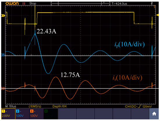
Figure 13.
the waveforms of primary current (blue) secondary current (orange).
The maximum value of the primary current is 22.43 A, and the maximum value of the secondary current is 12.75 A. The secondary current is continuous, and the fluctuation is smaller than the primary current.
5.2. Power Control
As discussed in Section 3.3.2, power can be controlled by energy injection period τ1. Figure 14 shows the experimental results of output power varying with τ1 under different coupling coefficients. The coupling coefficient is selected as k = 0.1, 0.2, 0.3. When τ1 = 40 μs, the output powers are 181.1 W, 171.6 W, and 167.1 W. When τ1 = 60 μs, the output powers are 379 W, 356.7 W, and 335.8 W. The results show that there is a linear relation between the output power and the energy injection period τ1. Under the same τ1 condition, the output power decreases slightly as k increases. The reason of this phenomenon is that the increase of k will lead to the decrease of leakage inductance and increase of the excitation inductance. The increase of excitation inductance results in a decrease of ip, and finally a decrease of output power.
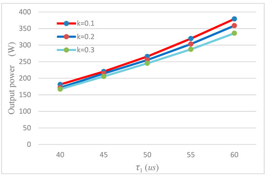
Figure 14.
Output power versus the energy injection period τ1 under condition of UDC = 300 V and R = 10 Ω.
The experimental results of output power varying with τ1 under different load, R are shown in Figure 15. It can be seen that there is still a good linearity between the output power and τ1. Using the curve of R = 10 Ω as an example. When τ1 = 40 μs, the output power is 171.6 W; when τ1 = 60 μs, the output power is 361.7 W. This curve is consistent with the curve of k = 0.2 in Figure 15. The output power varies slightly with the load R. When τ1 = 40 μs, the output power variation Δ, caused by varying R from 5 to 20, is 6 W, and when τ1 = 60 μs, the corresponding output power variation Δ is 26 W, i.e., the output power is slightly affected by the load R.
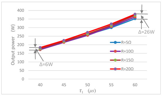
Figure 15.
Output power versus the energy injection period τ1 under condition of UDC = 300 V and k = 0.2.
The experimental results of total efficiency (UDC-load) versus the energy injection period τ1 are shown in Figure 16. It can be seen from Figure 16 that when τ1 = 45 μs, R = 15 Ω, the output is the lowest, which is 84.8%, and when τ1 = 40 μs, R = 5 Ω, the output is the lowest, which is 80.9%. The results of Figure 16 show that energy injection time has little effect on efficiency.
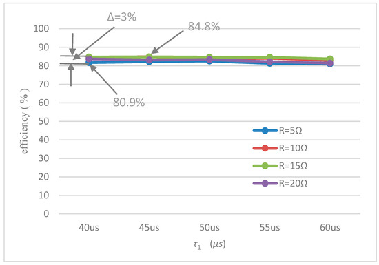
Figure 16.
Total efficiency (UDC-load) versus the energy injection period τ1 under condition of UDC = 300 V and k = 0.2.
5.3. Soft Switching
The driving voltage ug1, voltage drop uds1 of S1 and ip are shown in Figure 17. In Figure 17, ug1 changes from low lever to high lever in time margin Tm1 to turn on S1. In this time margin, uds1 is zero, therefore, S1 is turned on under ZVS condition. Similarly, ug1 changes from high to low level in time margin Tm2 to turn off S1, and in Tm2, uds1 is zero too. Therefore, S1 is turned off under ZVS condition. These results show that the switching operation of the IIEIFR converter does not need to be carried out at the current zero-crossing point but in a certain time slot to achieve soft switching condition. This feature reduces the complexity and difficulty of the control strategy.
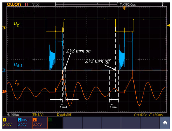
Figure 17.
Experimental results of soft switching condition of IIEIFR converter.
5.4. Power and Efficiency
The experimental results of the relationship between the efficiency and coupling coefficient k are shown in Table 4. In Table 4, k is represented by air gap, and the relationship of air gap and k is shown in Figure 9. In the experiment, power analyzer (Yokogawa-WT300) was used to collect efficiency data. Considering that coil copper resistance, core loss and other factors will affect the efficiency of the magneto-electric system [34], and the experiment is to investigate the performance of the IIEIFR converter, it is necessary to eliminate the influence of the magneto-electric system in this paper. In Table 4, Pin is the input power of the converter, Pop is the output power of the converter (measured at the input side of the primary coil), Pos is the output power of the magneto-electric system (measured at the load). ηp is the converter efficiency which is obtained by dividing Pop by Pin. Obviously, this is the efficiency after removing the influence of the magneto-electric system. ηs is the total efficiency, which is obtained by dividing Pos by Pin, which includes the effect of magneto-electric system.
Table 4.
Output power versus coupling coefficients.
As the air gap changes from 5 cm to 15 cm, the converter efficiency, ηp, is kept above 96.84%, and the highest is 98.79% in the air gap of 9cm. This result confirms the high efficiency characteristic of the IIEIFR converter, and the high efficiency may be attributed to the soft switching operation, lower energy frequency than the resonance frequency and no power backflow to the source. In addition, this result means that the efficiency of the IIEIFR converter is slightly affected by the air gap (coupling coefficient).
The total efficiency ηs is less than the converter efficiency ηp, when the air gap is 5 cm, ηs is 88.46% and when air gap is 15 cm, ηs is 80.31%. Since the focus of this paper is on the research of IIEIFR converter, not to optimize the system, therefore, the magneto-electric system used in this experiment is not optimal. The efficiency of the system may be improved by using pads with a higher quality factor, for example, using pads with a quality factor higher than 500 [32]. In addition, the results also show that the total efficiency of the system decreases with the increase of the air gap, and that is due to the decrease of the efficiency of the magneto-electric system with the air gap.
6. Conclusions
A prototype of IPT converter based on IIEIFR control strategy was built to drive the IPT system in a wide air-gap range. Both simulations and experiments verify that the IIEIFR system can decouple the converter from the resonant network, and the power can be controlled independently by the energy injection period. The experimental results show that under the conditions of UDC = 300 V, k = 0.2 and R = 10 Ω, the output power can be controlled nearly linearly by the energy injection period in the range of 40–60 μs, and the output power changed from 181 W to 379 W. Since only the inductance is involved in the energy injection process, other parameters of the system have slight influences on the power control. It is verified by the experiment results that the load and coupling coefficient have slight influence on the power control.
In the tested air-gap range, the converter efficiency is maintained above 96.84%, with a maximum of 98.79%, which shows the high efficiency characteristic of the IIEIFR converter. The total efficiency will be affected by the performance of the magneto-electric system. Within the test range, the total efficiency decreases from 88.46% to 80.31% with the increase of the air gap.
The presented control strategy has two time margins for state transitions under ZVS conditions, which can reduce the control difficulty of the circuit. Simulations and experiments show that when the resonant frequency is 6.8 kHz, the switches in the prototype have time margins of 28.5 μs and 73.7 μs for turning on and off, respectively.
Author Contributions
Conceptualization, L.C.; methodology, L.C.; software, J.H.; validation, L.C., J.H. and Z.L.; formal analysis, W.C., J.H. and M.G.; investigation, L.C., J.H. and Z.L.; resources, W.C. and M.G.; data curation, L.C., J.H. and M.G.; writing—original draft preparation, L.C.; writing—review and editing, M.G.; visualization, M.G.; supervision, W.C.; project administration, W.C.; funding acquisition, W.C.
Funding
This research was funded by National Natural Science Foundation of China (NSFC), grant number 51777177; NSFC grant number 51707168; Key Projects of Fujian Collaborative Innovation Center for R&D of Coach and Special Vehicle, grant number 2016AYF002.
Conflicts of Interest
The authors declare no conflict of interest.
References
- Kim, C.G.; Seo, D.H.; You, J.S.; Park, J.H.; Cho, B.H. Design of a Contactless Battery Charger for Cellular Phone. IEEE Trans. Ind. Electron. 2001, 48, 1238–1247. [Google Scholar] [CrossRef]
- Lu, Y.; Ma, D.B. Wireless Power Transfer System Architectures for Portable or Implantable Applications. Energies 2016, 9, 1087. [Google Scholar] [CrossRef]
- Wu, H.H.; Gilchrist, A.; Sealy, K.D.; Bronson, D. A High Efficiency 5 kW Inductive Charger for EVs Using Dual Side Control. IEEE Trans. Ind. Inform. 2012, 8, 585–595. [Google Scholar] [CrossRef]
- García, X.T.; Vázquez, J.; Roncero-Sánchez, P. Design, Implementation Issues and Performance of an Inductive Power Transfer System for Electric Vehicle Chargers with Series–series Compensation. IET Power Electron. 2015, 8, 1920–1930. [Google Scholar] [CrossRef]
- Jiang, C.; Chau, K.T.; Liu, C.; Lee, C.H.T. An Overview of Resonant Circuits for Wireless Power Transfer. Energies 2017, 10, 894. [Google Scholar] [CrossRef]
- Ibrahim, M.; Pichon, L.; Bernard, L.; Razek, A.; Houivet, J.; Cayol, O. Advanced Modeling of a 2-kw Series-series Resonating Inductive Charger for Real Electric Vehicle. IEEE Trans. Veh. Technol. 2015, 64, 421–430. [Google Scholar] [CrossRef]
- Hwang, K.; Cho, J.; Kim, D.; Park, J.; Kwon, J.H.; Kwak, S.I.; Park, H.H.; Ahn, S. An Autonomous Coil Alignment System for the Dynamic Wireless Charging of Electric Vehicles to Minimize Lateral Misalignment. Energies 2017, 10, 315. [Google Scholar] [CrossRef]
- Villa, J.L.; Sallan, J.; Sanz Osorio, J.F.; Llombart, A. High-misalignment tolerant compensation topology for icpt systems. IEEE Trans. Ind. Electron. 2012, 59, 945–951. [Google Scholar] [CrossRef]
- Kan, T.; Nguyen, T.D.; White, J.C.; Malhan, R.K.; Mi, C.C. A new integration method for an electric vehicle wireless charging system using lcc compensation topology: Analysis and design. IEEE Trans. Power Electron. 2017, 32, 1638–1650. [Google Scholar] [CrossRef]
- Sohn, Y.H.; Choi, B.H.; Lee, E.S.; Lim, G.C.; Cho, G.H.; Rim, C.T. General unified analyses of two-capacitor inductive power transfer systems: Equivalence of current-source SS and SP compensations. IEEE Trans. Power Electron. 2015, 30, 6030–6045. [Google Scholar] [CrossRef]
- Moradewicz, A.J.; Kazmierkowski, M.P. Contactless energy transfer system with FPGA-controlled resonant converter. IEEE Trans. Ind. Electron. 2010, 57, 3181–3190. [Google Scholar] [CrossRef]
- Jesús, S.; Villa, J.L.; Andrés, L.; José, F.S. Optimal design of ICPT systems applied to electric vehicle battery charge. IEEE Trans. Ind. Electron. 2009, 56, 2140–2149. [Google Scholar] [CrossRef]
- Keeling, N.A.; Covic, G.A.; Boys, J.T. A unity power factor IPT pick-up for high power applications. IEEE Trans. Ind. Electron. 2010, 57, 744–751. [Google Scholar] [CrossRef]
- Kim, J.H.; Lee, I.O.; Moon, G.W. Analysis and design of a hybrid-type converter for optimal conversion efficiency in electric vehicle chargers. IEEE Trans. Ind. Electron. 2017, 64, 2789–2800. [Google Scholar] [CrossRef]
- Choi, S.Y.; Gu, B.W.; Jeong, S.Y.; Rim, C.T. Advances in wireless power transfer systems for roadway-powered electric vehicles. IEEE J. Emerg. Sel. Top. Power Electron. 2014, 3, 18–36. [Google Scholar] [CrossRef]
- Zheng, C.; Ma, H.; Lai, J.S.; Zhang, L. Design Considerations to Reduce Gap Variation and Misalignment Effects for the Inductive Power Transfer System. IEEE Trans. Power Electron. 2015, 30, 6108–6119. [Google Scholar] [CrossRef]
- Cirimele, V.; Diana, M.; Freschi, F.; Mitolo, M. Inductive power transfer for automotive applications: State-of-the-art and future trends. IEEE Trans. Ind. Appl. 2018, 54, 4069–4079. [Google Scholar] [CrossRef]
- Mi, C.C.; Buja, G.; Choi, S.Y.; Rim, C.T. Modern advances in wireless power transfer systems for roadway powered electric vehicles. IEEE Trans. Ind. Electron. 2016, 63, 6533–6545. [Google Scholar] [CrossRef]
- Matysik, J.T. The Current and Voltage Phase Shift Regulation in Resonant Converters with Integration Control. IEEE Trans. Ind. Electron. 2007, 54, 1240–1242. [Google Scholar] [CrossRef]
- Gati, E.; Kampitsis, G.; Manias, S. Variable Frequency Controller for Inductive Power Transfer in Dynamic Conditions. IEEE Trans. Power Electron. 2017, 32, 1684–1696. [Google Scholar] [CrossRef]
- Matysik, J.T. A New Method of Integration Control with Instantaneous Current Monitoring for Class D Series-Resonant Converter. IEEE Trans. Ind. Electron. 2006, 53, 1564–1576. [Google Scholar] [CrossRef]
- Moghaddami, M.; Sundararajan, A.; Sarwat, A.I. A Power-Frequency Controller with Resonance Frequency Tracking Capability for Inductive Power Transfer Systems. IEEE Trans. Ind. Appl. 2018, 54, 1773–1783. [Google Scholar] [CrossRef]
- Miller, J.M.; Onar, O.C.; Chinthavali, M. Primary-side power flow control of wireless power transfer for electric vehicle charging. IEEE J. Emerg. Sel. Top. Power Electron. 2015, 3, 147–162. [Google Scholar] [CrossRef]
- Madawala, U.K.; Neath, M.; Thrimawithana, D.J. A power–frequency controller for bidirectional inductive power transfer systems. IEEE Trans. Ind. Electron. 2013, 60, 310–317. [Google Scholar] [CrossRef]
- Berger, A.; Agostinelli, M.; Vesti, S.; Oliver, J.A.; Cobos, J.A.; Huemer, M. A wireless charging system applying phase-shift and amplitude control to maximize efficiency and extractable power. IEEE Trans. Power Electron. 2015, 30, 6338–6348. [Google Scholar] [CrossRef]
- Dede, E.J. Improving the Efficiency of IGBT Series-resonant Inverters using Pulse Density Modulation. IEEE Trans. Ind. Electron. 2011, 58, 979–987. [Google Scholar] [CrossRef]
- Fujita, H.; Akagi, H. Pulse-density-modulated Power Control of a 4 kw, 450 kHz Voltage-source Inverter for Induction Melting Applications. IEEE Trans. Ind. Appl. 1996, 32, 279–286. [Google Scholar] [CrossRef]
- Li, H.L.; Hu, A.P.; Covic, G.A. Development of a Discrete Energy Injection Inverter for Contactless Power Transfer. In Proceedings of the 2008 3rd IEEE Conference on Industrial Electronics and Applications, Singapore, 3–5 June 2008; pp. 1757–1761. [Google Scholar] [CrossRef]
- Li, H.L.; Hu, A.P.; Covic, G.A. A Direct AC–AC Converter for Inductive Power-Transfer Systems. IEEE Trans. Power Electron. 2012, 27, 661–668. [Google Scholar] [CrossRef]
- Chen, L.; Hong, J.; Guan, M.; Wu, W.; Chen, W. A Power Converter Decoupled from the Resonant Network for Wireless Inductive Coupling Power Transfer. Energies 2019, 12, 1192. [Google Scholar] [CrossRef]
- Wang, C.S.; Covic, G.A.; Stielau, O.H. Power transfer capability and bifurcation phenomena of loosely coupled inductive power transfer systems. IEEE Trans. Ind. Electron. 2004, 51, 148–157. [Google Scholar] [CrossRef]
- Kamineni, A.; Covic, G.A.; Boys, J.T. Self-Tuning Power Supply for Inductive Charging. IEEE Trans. Power Electron. 2017, 32, 3467–3479. [Google Scholar] [CrossRef]
- Esteve, V.; Jordan, J.; Sanchis-Kilders, E.; Dede, E.; Maset, E.; Ejea, J. Enhanced pulse-density-modulated power control for high frequency induction heating inverters. IEEE Trans. Ind. Electron. 2015, 62, 6905–6914. [Google Scholar] [CrossRef]
- Lin, F.Y.; Covic, G.A.; Boys, J.T. Evaluation of Magnetic Pad Sizes and Topologies for Electric Vehicle Charging. IEEE Trans. Power Electron. 2015, 30, 6391–6407. [Google Scholar] [CrossRef]


© 2019 by the authors. Licensee MDPI, Basel, Switzerland. This article is an open access article distributed under the terms and conditions of the Creative Commons Attribution (CC BY) license (http://creativecommons.org/licenses/by/4.0/).