Abstract
High bandwidths and accurate current controls are essential in high-performance permanent magnet synchronous (PMSM) servo drives. Compared with conventional proportional–integral control, deadbeat current control can considerably enhance the current control loop bandwidth. However, because the deadbeat current control performance is strongly affected by the variations in the electrical parameters, tuning the controller gains to achieve a satisfactory current response is crucial. Because of the prompt current response provided by the deadbeat controller, the gains must be tuned within a few control periods. Therefore, a fast online current loop tuning scheme is proposed in this paper. This scheme can accurately identify the controller gain in one current control period because the scheme is directly derived from the discrete-time motor model. Subsequently, the current loop is tuned by updating the deadbeat controller with the identified gains within eight current control periods or a speed control period. The experimental results prove that in the proposed scheme, the motor current can simultaneously have a critical-damped response equal to its reference in two current control periods. Furthermore, satisfactory current response is persistently guaranteed because of an accurate and short time delay required for the current loop tuning.
1. Introduction
A modern servo motor drive usually includes current, speed, and position control loops. In general, the current loop bandwidth is considerably higher than the bandwidth of the speed and position loops. Therefore, a current loop with a high bandwidth can fundamentally enhance the performance of the servo motor drive.
When the current loop is implemented with a digital signal processor (DSP), because of the limited computation capability, the calculated voltage command requires one control period delay for the pulse width modulation (PWM) module to output voltage to the motor. This time delay causes an underdamped or unstable current response when a proportional–integral (PI) controller is used for motor current regulation [1,2,3,4]. The discretized PI controller directly designed in the z-domain has been proposed in [3,4]; however, limited improvement in the current loop bandwidth was achieved and current overshoots were persistent. To eliminate the influences of the time delay, schemes based on the predictive current control [5,6,7,8,9,10,11] and deadbeat current control [12,13,14,15,16,17] have been proposed. The predictive current controller generates the optimal voltage vector by minimizing a specific cost function. This voltage vector allows the motor current to reach its reference value as fast as possible with minimum overshoot. Deadbeat current control is well-known for its zero overshoot, zero steady-state error, and minimum rise time characteristics. Consequently, the motor current can reach its reference value with minimum control periods without overshoot. Compared with predictive current control, deadbeat control is simple to implement and requires less computation. However, its performance is parameter-dependent, as reported in [15,16,17]. In particular, inductance is sensitive to the current level. Online controller gain tuning is an effective method to mitigate the effects of parameter variations.
Numerous online electrical parameter identification strategies have been proposed. The observer-based methods in [18,19,20,21] identify the parameters by converging the error between the sampled and estimated current to zero. In [18], the identified inductance was used for the predictive current controller to improve the robustness of the current loop. Observer-based methods often require long execution times because of the delay of the observer and may encounter stability problems. The authors in [22,23,24] performed the recursive least-square (RLS) algorithm to identify electrical parameters. The motor model was used to develop the RLS algorithm. Then, the parameters were identified by minimizing the discrepancy between the sampled and calculated current. Although the latency caused by the observer does not exist in RLS-based methods, accurately identifying the parameters in a few control periods is still difficult. In addition, the electrical parameters are generally identified instead of the controller gains in these methods. However, the effect caused by the parameter mismatch can be treated as a disturbance to the current controller. To compensate for this disturbance, the compensation voltage, which was obtained through the disturbance observer in [12,17] and through adaptive control in [25], is added to the current loop. Despite their effectiveness, the schemes in [17,25] involve a complex design procedure to achieve satisfactory performance.
In this study, a deadbeat current controller was designed to enhance the current loop bandwidth for its simple implementation. A novel online current loop tuning strategy is proposed to reduce the effect of parameter variations. The proposed method is simple and effective because the method is directly derived from the discrete-time motor model. In addition, the proposed method directly identifies the gains of the deadbeat controller instead of the electrical parameters. After the controller gains are identified, the gains are averaged to further improve accuracy. Then, the current loop is tuned by updating the deadbeat controller with the average gains.
2. Discrete-Time Motor Model
The stator voltage of a PMSM in the rotor reference frame can be expressed as follows:
where , , , and are the q- and d-axis voltages and currents, respectively; Lqs and Lds are the q- and d-axis inductance, respectively; rs, ωr, and λm are the phase resistance, rotor electrical speed, and magnet flux, respectively; and s denotes the Laplace operator. When the current loop and PWM function of the PMSM are implemented digitally, a time delay is inevitably introduced. Figure 1 displays the time sequence of the current sampling, voltage command calculation, and voltage command output, where Ts is the sampling period of the motor currents and the control period of the current loop. As depicted in Figure 1, the voltage command is calculated at t0 and outputs to the PWM module at t0 + Ts. Then, the voltage command is activated by the PWM module and held for one sampling period during t0 + Ts to t0 + 2Ts. The motor current induced by the corresponding voltage command is then sampled at t0 + 2Ts. Therefore, a time delay of two sampling periods is generated in the current loop. The PWM function and calculation delay can be modeled together by using a zero-order hold involving one sampling period delay. Accordingly, the stator voltage in Equation (1) can be discretized as follows:
where Z{} is the Z-transform; the model gains Amq and Bmq are and (1 − Amq)/rs, respectively; and the model gains Amd and Bmd are and (1 − Amd)/rs, respectively. Because the back-EMF and cross-coupling voltages are approximately constant within one control period, these voltages are assumed to be decoupled from the current controller and are not represented in Equations (2) and (3). The q- and d-axis decoupling voltages, namely vqff and vdff, respectively, are derived from Equation (1) by using the estimated electrical parameters and rotor speed in the following expression:
where “^” denotes the estimated quantity.
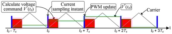
Figure 1.
Time sequence for current sampling, voltage command calculation, and output, where PWM is pulse-width modulation.
3. Overall Control System
3.1. Servo Control System
Figure 2 illustrates the overall servo control system, where van, vbn, and vcn are the phase voltages; θm, θr, and ωm denote the mechanical position, electrical angle, and speed, respectively; and “*” denotes the command value. The motor current is regulated using a deadbeat current controller. The classical proportional position with proportional-plus-integral velocity (P-PI) control is implemented to regulate the motor speed and position [26]. The bandwidths of the speed loop and position loop are set as 100 and 10 Hz, respectively. The proposed online current loop tuning algorithm continuously tunes the gains in the current loop to achieve a satisfactory current response. The variables associated with the online tuning are defined in the following text.
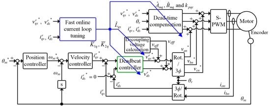
Figure 2.
Block diagram of servo control system with the proposed online current loop tuning strategy.
3.2. Dead-Time Compensation
High-performance servo motor drives generally include dead-time compensation. The voltage error caused by the dead time can be measured through the steady-state voltage command and current feedback [27]. The voltage error at different phase currents for the inverter used in this study is depicted in Figure 3. The configuration of the motor drive is listed in Table A1. The voltage error saturates when the magnitude of the phase current is higher than 1 A. After the voltage error is calculated with the phase current feedback, dead-time compensation is performed by adding the voltage error to the current loop, as depicted in Figure 2.
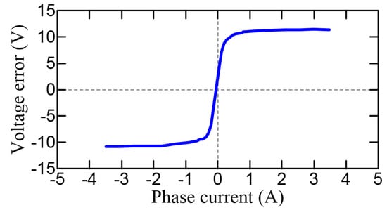
Figure 3.
The voltage error caused by the dead-time at different phase current.
The time delay in the current loop can degrade the effectiveness of dead-time compensation. To mitigate the influence of this time delay, the estimated phase current is used to calculate the voltage error. Figure 4 illustrates the proposed current estimator. A PI controller is used to reduce the error between the sampled and estimated current. By ignoring the PI controller, the estimated current can be expressed as follows:
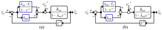
Figure 4.
The proposed (a) q-axis and (b) d-axis current estimator.
When the parameters are correct, the estimated current approximates the current sampled at the (k + 2)th sampling instant, which is induced by and . An operator z−2 is added in the feedback path of the estimator because the estimated current is from two sampling periods before the present sampled current. Then, the estimated phase current can be calculated as follows:
The pole-zero cancelation technique is used to design the PI controller of the current estimators. By canceling the plant pole with the controller zero, the proportional gain kpqc and kpdc are calculated as follows:
where kiqc and kidc are the integral gains. Figure 5 shows the damping ratio and bandwidth of the current estimator for various kiqc values. The bandwidth of the current estimator is determined from the integral gain, and the proportional gains are then calculated using Equations (8) and (9).
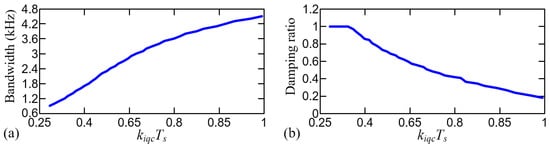
Figure 5.
The (a) bandwidth and (b) damping ratio of the current estimator at different integral gain.
In this study, the bandwidth of the current estimator was set to 900 Hz because this can simultaneously ensure that the estimated current strictly follows the sampled feedback current and the estimator predicts the sampled current accurately. In addition, the current estimator has a critical-damped response.
4. Deadbeat Current Controller
When a conventional PI controller is used to regulate the motor current, the time delay in the control loop can cause stability problems because of the degraded phase margin. Consequently, the current loop bandwidth is limited to maintaining an acceptable overshoot on the motor current. To enhance the bandwidth of the current loop to its theoretical maximum, a deadbeat current controller was developed in this study.
Deadbeat Controller Design
Figure 6 depicts the schematics of the q- and d-axis current control loops with the deadbeat controller, where Cq(z) and Cd(z) are the deadbeat controllers for the q- and d-axes, respectively. Deadbeat controller design is conducted entirely in the z-domain. All the closed-loop poles are placed at the origin in the z-domain. The q-axis transfer function is expressed as follows:
where the numerator h(z) provides an additional degree of freedom for the controller design and n is the number of poles. The q-axis current should strictly follow the command value without a steady-state error. By applying the finite-value theorem to Equation (10), the following result is obtained:
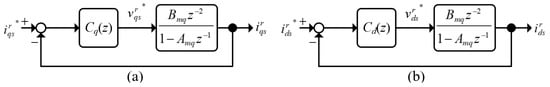
Figure 6.
(a) q-axis and (b) d-axis current loop with the deadbeat controller when the motor is at standstill.
For convenience, h(z) is set as 1. The difference form of Equation (10) can be derived as follows:
The results indicate that the q-axis current lags the command value by n control periods when h(z) = 1. Except for the zero steady-state error, the q-axis current can also reach the command value without an overshoot.
According to Equation (10) and the relation h(z) = 1, the deadbeat controller Cq(z) can be derived using the estimated electrical parameters. The deadbeat controller Cq(z) is expressed as follows:
The transfer function of the q-axis voltage command is given as follows:
To satisfy the causality, the following inequality must be satisfied:
where deg{} denotes the highest order of the polynomial. When n is selected to be 2 and the parameters are perfectly matched, the q-axis current can attain the steady-state and equal the command value in two control periods. In addition, the voltage command can attain the steady state in two control periods after the current command changes. Therefore, Cq(z) is modified as follows:
The q-axis voltage command at the kth control instant can be derived from (16) as follows:
where , and . Similarly, the deadbeat controller Cd(z) can be derived as follows:
The d-axis voltage command at the kth sampling instant is expressed as follows:
where , and . Figure 7 depicts the detailed schematics of Cq(z) and Cd(z) with the decoupling voltage and voltage limitation.
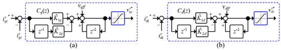
Figure 7.
Block diagram of the deadbeat controller with the decoupling voltage and voltage limitation block, (a) Cq(z) and (b) Cd(z).
5. Simulation Results
A 400-W servo motor was used in the simulation. The motor parameters are listed in Table A2. The drive losses were ignored in the simulation. The voltage command was limited to half of the DC voltage because sinusoidal PWM was implemented, as illustrated in Figure 7. Because the d-axis current is expected to have a similar response as the q-axis current, only the q-axis current simulation results are presented.
5.1. Results with Correct Motor Parameters
Figure 8 and Figure 9 illustrate the q-axis current, current command, and voltage command when the current steps from 0 to 1 A and from 0 to 4 A, respectively, when the motor is at standstill. As depicted in Figure 8, the q-axis current does not exhibit overshoot and is exactly equal to the command value in two control periods after the current command changes. The voltage command is generated immediately after the current command changes. The voltage commands at the kTs and (k + 1)Ts control periods can be calculated as follows:
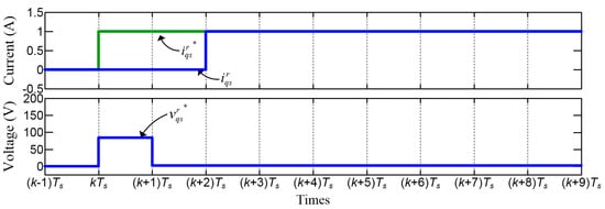
Figure 8.
The simulated q-axis current, current command, and voltage command when the current command steps from 0 A to 1 A.
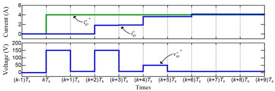
Figure 9.
The simulated q-axis current, current command, and voltage command when the current command steps from 0 A to 4 A.
Note that these command values are less than half of the DC supply.
Conversely, as depicted in Figure 9, the q-axis current increases slowly and requires approximately six control periods to attain the command value because the voltage required for the current to increase from 0 to 4 A in one control period exceeds the command limit. The voltage command saturates several times before the q-axis current reaches its command value, which is in agreement with the control law presented in Equation (17). The actual rise time is dependent on the motor inductance.
Figure 10 illustrates the frequency response of the deadbeat controller without voltage limitations. The current loop gain is 0 dB at low frequencies and is flat until the Nyquist frequency. This indicates that the current can follow its command without overshoot and steady-state error. However, the phase lag increases with frequency. The phase margin decreases to 0 at 4.575 kHz. Therefore, the maximum theoretical bandwidth of the proposed deadbeat controller is one-fourth of the control frequency.
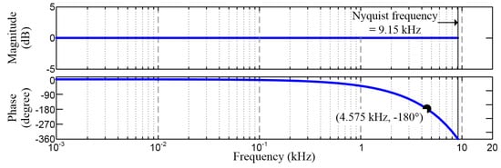
Figure 10.
The frequency response of the deadbeat current controller without voltage limitation.
5.2. Results with Parameter Mismatch
The phase resistance and q- and d-axis inductances are required to design a deadbeat controller. The deadbeat controller performance is dependent on the accuracy of the estimated electrical parameters. Figure 11 and Figure 12 display the dominant poles of the q-axis current loop in the z-domain and the corresponding q-axis current response when the current command steps from 0 to 1 A and the phase resistance varies 50% and 150% from its nominal value, respectively. The figures indicate that the poles remain near the origin regardless of the variations in the phase resistance. The q-axis current can still reach its command value in two control periods; however, marginal overshoot is observed. This implies that the influence of the resistance mismatch to the deadbeat controller is trivial. However, the q-axis current depicted in Figure 11 is marginally lower than its command value at the steady state because the resistance is smaller than its nominal value. Conversely, the q-axis current illustrated in Figure 12 is marginally higher than its command value at the steady state because the resistance is larger than its nominal value.
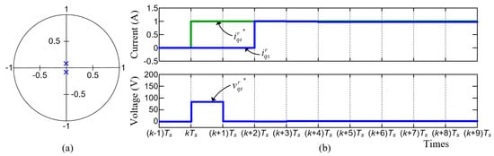
Figure 11.
(a) The dominant poles and (b) simulated q-axis current and voltage command with when the current command steps from 0 A to 1 A. The motor is at standstill.
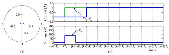
Figure 12.
(a) The dominant poles and (b) simulated q-axis current and voltage command with when the current command steps from 0 A to 1 A. The motor is at standstill.
Figure 13 and Figure 14 illustrate the dominant poles of the q-axis current loop and the corresponding q-axis current response when the current command steps from 0 to 1 A and the q-axis inductance varies 50% and 120% from its nominal value, respectively. In contrast to the results depicted in Figure 11 and Figure 12, the variations in the inductance considerably deteriorate the system performance. As depicted in Figure 13, the current response becomes overdamped when the inductance is smaller than its nominal value because the poles mitigate toward the unit circle along the real axis. However, in Figure 14, the current response becomes underdamped when the inductance is larger than its nominal value because the poles mitigate toward the unit circle along the imaginary axis. Although no steady-state error is observed, the transient response of the q-axis current is considerably affected. In addition, the current loop can become unstable if the poles mitigate outside the unit circle because of the mismatched inductance.
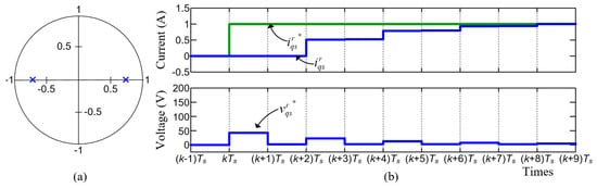
Figure 13.
(a) The dominant poles and (b) simulated q-axis current and voltage command response with when the current command steps from 0 A to 1 A, the motor is at standstill.
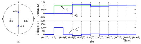
Figure 14.
(a) The dominant poles and (b) simulated q-axis current and voltage command response with when the current command steps from 0 A to 1 A, the motor is at standstill.
6. Online Current Loop Tuning
The deadbeat controller performance is considerably affected by parameter mismatch because the voltage command is directly related to the voltage drop on the inductance and resistance. In this study, a novel online current loop tuning strategy was developed to preserve the deadbeat controller performance. Only the q-axis current loop is discussed because similar results can be obtained for the d-axis current loop.
6.1. Controller Gain Identification
From Equation (2), the q-axis current sampled at the kth and (k − 1)th control instants can be expressed as follows:
Equation (22) can be rearranged as follows:
where K1q and K2q are defined as and , respectively. Because the voltage error caused by the dead-time is satisfactorily compensated, the controller gains K1q and K2q can be reasonably estimated using the command values, which are expressed as follows:
To solve Equation (24), the determinant of the inverse matrix must be a nonzero value. This condition is expressed as follows:
As presented in Equation (24), the controller gains can be estimated using the sampled currents and voltage commands.
6.2. Estimation Accuracy Improvement
The controller gains cannot be identified in the steady state because is 0. In addition, although the current ripples caused by the speed and position controller or current sensor noise yield nonzero , these currents cannot be used to identify controller gains because they have a low correlation with the motor parameters and consequently a low signal-to-noise-ratio (SNR). Figure 15a depicts a steady-state q-axis current with a current ripple. Although the current ripple is unpredictable in practice, the ripple is modeled as a square wave with an amplitude of Δi for convenience of analysis. Then, with the current ripple is calculated as follows:
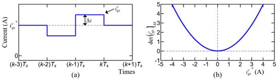
Figure 15.
(a) Steady-state q-axis current with current ripple, and (b) versus current command.
Figure 15b depicts a plot of versus the q-axis current command when Δi is set as 10% of the command value. It can be seen that increases with the current level. Therefore, a threshold for must be set to avoid identification error in the steady state. Accordingly, controller gain identification is performed only when the following condition is satisfied:
where is the threshold value. In general, the threshold value can be tuned through experiments.
The identification accuracy can be further improved by averaging the controller gains calculated in the last m control periods. In addition, each identified gain is weighted using its . The averaged controller gains are calculated as follows:
Because the average controller gain is dominated by the identified gain with higher , the identification accuracy improves.
After the average controller gains are calculated, the model gains can be determined as follows:
Because the effect of resistance variation on the current response is trivial, the estimated q-axis inductance can be approximated as follows:
The model gains and as well as the estimated d-axis inductance can be obtained similarly. As depicted in Figure 1, the estimated inductances and model gains are used for the decoupling voltage calculation and dead-time compensation, respectively.
6.3. Identification When Voltage Command Is Limited
Vmax depends on the DC voltage and the dead-time of the inverter. The motor used in this study has almost identical q- and d-axis inductances. Thus, the d-axes current is controlled to 0 to generate the required torque with a minimum stator current. Consequently, the d-axis voltage approximates to the decoupling voltage and the steady-state q-axis voltage can be calculated using Equation (34) when the stator voltage saturates to Vmax.
Subsequently, the voltage command used to identify the controller gains when the voltage is limited is obtained as follows:
6.4. Gain Update Method
Figure 16 illustrates the timing for identifying and updating the gains in a deadbeat controller and current estimator, where the green bar denotes the execution of the current control and the blue bar denotes the execution of the speed and position control. Because the d-axis current is controlled to 0, only the gains in the q-axis current loop are identified. However, because , the gains in Cd(z) and the d-axis current estimator are set equal to the corresponding q-axis values. The controller gains are identified when the current control loop is executed. Because the current control executes eight times faster than the speed and position control, at most eight controller gains are identified before the next speed control is executed. Then, , , , , , and kpqc are calculated using Equations (8) and (28)–(32) when the speed control is executed. Subsequently, the gains in the deadbeat controller and the parameters in the current estimator are updated in the next execution of the current control because the motor current generally reaches steady state at this instant. The PI controller in the current estimator is updated two control periods after the model gain is updated because the sampled current is two control periods behind the estimated current.
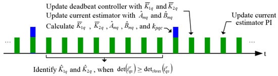
Figure 16.
Time sequence of the gain identification, calculation and updating.
7. Experimental Results
A 400-W servo motor was used for experimental verifications. The parameters of the motor are provided in Table A1. Figure 17 illustrates the experimental system. The proposed online current loop tuning scheme is implemented using a Texas Instruments TMS320F28335 DSP. The detailed configuration of the drive is detailed in Table A2. In this study, Vmax was set to 139 V to account for the losses caused by the dead time. The motor position and speed were measured using an encoder with a resolution of 2500 pulse/rev.
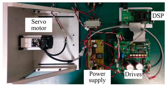
Figure 17.
Experimental system.
The experimental results shown in Figure 18, Figure 19, Figure 20 and Figure 21 were obtained without the online current loop tuning algorithm. Figure 18 illustrates the q-axis current and voltage command response when the current increased from 0 to 1 A and from 0 to 4 A, respectively, when the motor was at standstill. The voltage command was less than the limit for the 1 A step but exceeded the limit for the 4 A step. As depicted in Figure 18a, the q-axis current was exactly two current control periods behind the command value. Furthermore, overshoot and steady state error were not observed for the current. However, the q-axis current presented in Figure 18b required approximately seven control periods to reach the command value because the voltage was limited to 139 V. These results highly concur with the simulation results described in Section 5. Thus, the effectiveness of the deadbeat current controller was verified.
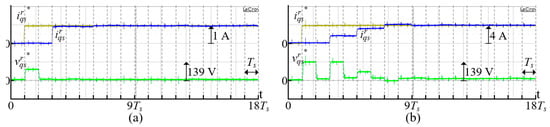
Figure 18.
q-axis current and voltage when the motor is at standstill and the current command steps from (a) 0 A to 1 A, (b) 0 A to 4 A.
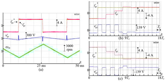
Figure 19.
q-axis current, voltage, and speed when the motor cycles between −3000 rpm and 3000 rpm with step current command, (a) complete waveform, (b) amplified view when current command steps from −4 A to 4 A, (c) amplified view when current command steps from 4 A to −4 A.
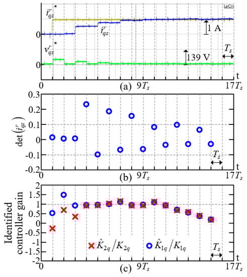
Figure 20.
Current command steps from 0 A to 1 A when the motor is at standstill and , (a) q-axis current and voltage command, (b) , (c) normalized identified controller gains.
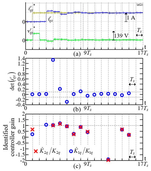
Figure 21.
Current command steps from 0 A to 1 A when the motor is at standstill and , (a) q-axis current and voltage command, (b) , (c) normalized identified controller gains.
Figure 19a demonstrates the q-axis current, voltage, and speed response when the motor had rotation speeds between −3000 and 3000 rpm. The q-axis current followed the command value closely regardless of the motor speed. Figure 19b,c depicts the amplified views of the situation when the current increased from −4 to 4 A and decreased from 4 to −4 A, respectively. The deadbeat controller produced pulse-wise voltage because the stator voltage was limited. Although the voltage command had an opposite polarity to that of the decoupling voltage, the q-axis current required seven control periods to reach the command value. According to the aforementioned results, the performance of the deadbeat controller was independent of the motor speed. However, a marginal current overshoot is observed in Figure 18b and Figure 19b,c because of the magnetic saturation.
Figure 20a and Figure 21a illustrate the q-axis current and voltage response when the current increased from 0 to 1 A as the estimated inductance was set as 50% and 120% of its nominal value, respectively. The experiments were performed when the motor was at standstill. As depicted in Figure 20a, when , the q-axis current became overdamped and required seven control periods to reach the command value. However, as depicted in Figure 21a, when , the q-axis current became underdamped and had an observable overshoot. The experimental results are similar to the simulation results presented in Section 5.
Figure 20b,c displays the calculated and controller gains for the transient response depicted in Figure 20a, respectively. Similarly, Figure 21b,c displays the calculated and controller gains for the transient response presented in Figure 21a, respectively. For convenience of observation, the controller gains were normalized by their nominal values. Moreover, only the gains within ±200% of their nominal value are displayed. As depicted in the aforementioned figures, a large current difference resulted in a high magnitude. Consequently, highly accurate gains were obtained because of a superior SNR. In general, the controller gain could be accurately identified for . The maximum error between the identified controller gains and their nominal values were within 16%. Moreover, the proposed identification method could identify the controller gains in one current control period provided was sufficiently large.
Figure 22 displays the speed, position, and current responses when the motor was controlled in the positioning mode. The motor moved forward to 11π and then back to 0. The maximum speed was 3000 rpm, which is the rated speed of the motor. Furthermore, the motor was accelerating and decelerating with its rated current. An observable position error was obtained only when the motor was accelerating and decelerating. In the following experiments, the waveforms in the acceleration region were amplified to examine the effectiveness of the online current loop tuning scheme. In addition, the lowest bound of for the controller gain calculation was set as 0.2 to ensure sufficient identification accuracy.
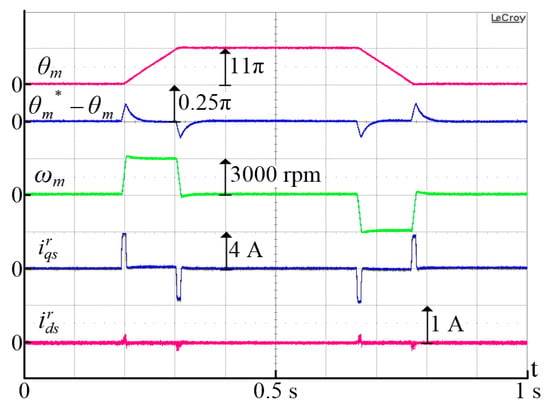
Figure 22.
Speed, position, and current waveforms when the motor is controlled in the positioning mode.
Figure 23a, Figure 24a, and Figure 25a depict the current response with , , and respectively, when online current loop tuning was deactivated. Conversely, Figure 23b, Figure 24b, and Figure 25b display the same waveforms but with online current loop tuning activated. The average controller gains were normalized by their nominal value for a clear observation. Figure 23a indicates that even with the correct inductance, overshoot and undershoot were observed for the q-axis current at high current levels because of the magnetic saturation. By contrast, as indicated in Figure 23b, no apparent overshoot was observed after online current loop tuning was activated.
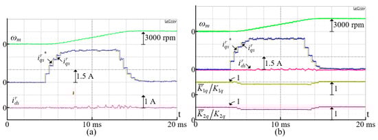
Figure 23.
The amplified current response in the acceleration region of Figure 23 with when the online current loop tuning is (a) de-activated and (b) activated.
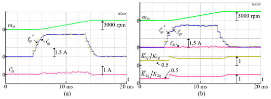
Figure 24.
The amplified current response in the acceleration region of Figure 23 with when the online current loop tuning is (a) de-activated and (b) activated.
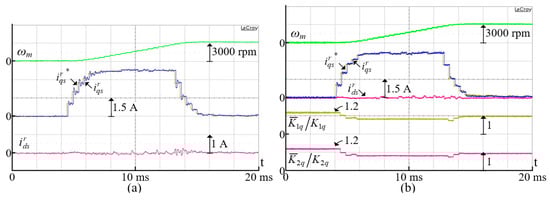
Figure 25.
The amplified current response in the acceleration region of Figure 23 with when the online current loop tuning is (a) de-activated and (b) activated.
As depicted in Figure 24a, because the estimated inductance was set to half of the nominal value, the q-axis current response became overdamped. In addition, the d-axis current had a marginal steady-state error. By contrast, as illustrated in Figure 24b, the q-axis current was tuned to reach its reference without overshoot within a speed control period and the d-axis current had no steady state error after online current loop tuning was activated. The q-axis current in Figure 25a exhibits considerable overshoot despite the current level because the q-axis inductance is 20% higher than its nominal value. This caused additional ripples to appear on the d-axis current. However, as depicted in Figure 25b, the overshoot was eliminated within a speed control period after online current loop tuning was activated. It can be observed in Figure 24b and Figure 25b that after the deadbeat controller is tuned by the proposed method, the required sampling period for current to reach its command value is reduced from nine to two sampling periods, and the overshoot on the current is reduced from 0.4 A to 0.09 A. These experimental results verify that the proposed method is effective and can greatly reduce the sensitivity of the deadbeat controller to the variations in inductance.
Figure 26 displays the measured and calculated frequency response of the q-axis deadbeat current controller. In the measurements, voltage was within the limit and the motor was at standstill. It can be seen that the current amplitude did not vary with frequency. However, the phase delay gradually increased with frequency. This is because the deadbeat controller was designed to reach its reference in two control periods, and the phase delay for two time periods was small at low frequencies but large at high frequencies.
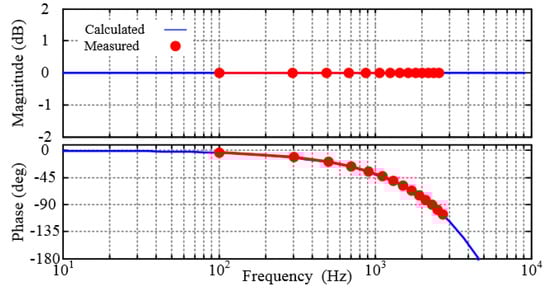
Figure 26.
The measured and the calculated frequency response of the deadbeat current controller.
8. Conclusions
In this study, we present an online controller gain tuning scheme for deadbeat current control. The experimental results verify that the motor current can reach its reference value without overshoot in two current control periods with the deadbeat controller and correct parameters. However, the current response can easily become overdamped or underdamped when the controller gains are calculated using incorrectly estimated inductances. The proposed online controller gain tuning scheme is derived on the basis of the discrete-time motor model. The experimental results indicate that the correct controller gains can be identified in one current control period, and the control loop is tuned in a speed control period. Consequently, the deadbeat controller can persistently control the motor current to its reference value in two sampling periods without overshoot irrespective of the inductance variations. Furthermore, the proposed scheme is easy to implement and requires limited computations.
Author Contributions
Conceptualization, Z.-C.Y., C.-H.H., and S.-M.Y.; methodology, Z.-C.Y. and C.-H.H.; software, C.-H.H.; validation, Z.-C.Y., C.-H.H., and S.-M.Y.; formal analysis, Z.-C.Y. and C.-H.H.; investigation, Z.-C.Y. and C.-H.H.; resources, S.-M.Y.; data curation, C.-H.H.; writing—original draft preparation, Z.-C.Y.; writing—review and editing, S.-M.Y.; visualization, Z.-C.Y.; supervision, S.-M.Y.; project administration, S.-M.Y.
Funding
This research received no external funding.
Conflicts of Interest
The authors declare no conflict of interest.
Appendix A

Table A1.
Main drive parameters.
Table A1.
Main drive parameters.
| Value | Unit | |
|---|---|---|
| DC voltage | 300 | V |
| Sampling period for current loop (Ts) | 55 | μs |
| Sampling period for speed and position loop | 440 | μs |
| Dead-time | 2 | μs |
Table A2.
Main motor parameters.
Table A2.
Main motor parameters.
| Value | Unit | |
|---|---|---|
| Rated speed/pole pairs | 3000/5 | rpm |
| Rated current | 4 | A |
| Magnet flux (λm) | 0.042 | Wb-turns |
| Stator resistance (rs) | 1.4 | Ω |
| d-axis inductance (Lds) | 4.46 | mH |
| q-axis inductance (Lqs) | 4.54 | mH |
References
- Bocker, J.; Beineke, S.; Bahr, A. On the Control Bandwidth of Servo Drives. In Proceedings of the 13th European Conference Power Electronics Applications, Barcelona, Spain, 8–10 September 2009; pp. 1–10. [Google Scholar]
- Huh, K.K.; Lorenz, R.D. Discrete-Time Domain Modeling and Design for AC Machine Current Regulation. In Proceedings of the Conference Record 42th IEEE/IAS Annual Meeting, New Orleans, LA, USA, 23–27 September 2007; pp. 2066–2073. [Google Scholar]
- Kim, H.; Degner, M.W.; Guerrero, J.M.; Briz, F.; Lorenz, R.D. Discrete-Time Current Regulator Design for AC Machine Drives. IEEE Trans. Ind. Appl. 2011, 46, 1425–1435. [Google Scholar]
- Yepes, A.G.; Vidal, A.; Malvar, J.; Lopez, O.; Jesus, D.G. Tuning Method Aimed at Optimized Setting Time and Overshoot for Synchronous Proportional-Integral Current Control in Electric Machines. IEEE Trans. Power Electron. 2014, 29, 3041–3054. [Google Scholar] [CrossRef]
- Andersson, A.; Thiringer, T. Assessment of an Improved Finite Control Set Model Predictive Current Controller for Automotive Propulsion Applications. IEEE Trans. Ind. Electron. 2019, 67, 91–100. [Google Scholar] [CrossRef]
- Cortes, P.; Kazmierkowski, M.P.; Kennel, R.M.; Quevedo, D.E.; Rodriguez, J. Predictive Control in Power Electronics and Drives. IEEE Trans. Ind. Electron. 2008, 55, 4312–4324. [Google Scholar] [CrossRef]
- Zhang, Y.; Xu, D.; Liu, J.; Gao, S.; Xu, W. Performance Improvement of Model-Predictive Current Control of Permanent Magnet Synchronous Motor Drives. IEEE Trans. Ind. Appl. 2017, 53, 3683–3695. [Google Scholar] [CrossRef]
- Lin, C.K.; Liu, T.H.; Yu, J.T.; Fu, L.C.; Hsiao, C.F. Model-Free Predictive Current Control for Interior Permanent-Magnet Synchronous Motor Based on Current Difference Detection Technique. IEEE Trans. Ind. Electron. 2014, 61, 667–681. [Google Scholar] [CrossRef]
- Lin, C.K.; Yu, J.T.; Lai, Y.S.; Yu, H.C. Improved Model-Free Predictive Current Control for Synchronous Reluctance Motor Drives. IEEE Trans. Ind. Electron. 2016, 63, 3942–3953. [Google Scholar] [CrossRef]
- Young, H.A.; Perez, M.A.; Rodriguez, J. Analysis of Finite-Control-Set Model Predictive Current Control with Model Parameter Mismatch in a Three-Phase Inverter. IEEE Trans. Ind. Electron. 2016, 63, 3100–3107. [Google Scholar] [CrossRef]
- Ahmed, A.A.; Koh, B.K.; Lee, Y.I. A Comparison of Finite Control Set and Continuous Control Set Model Predictive Control Schemes for Speed Control of Induction Motors. IEEE Trans. Ind. Informat. 2018, 14, 1334–1346. [Google Scholar] [CrossRef]
- Yang, H.; Zhang, Y.; Liang, J.; Xia, B.; Walker, P.D.; Zhang, N. Deadbeat Control Based on a Multipurpose Disturbance Observer for Permanent Magnet Synchronous Motors. IET Electr. Pwer Appl. 2018, 12, 708–716. [Google Scholar] [CrossRef]
- Isermann, R. Digital Control System; Springer: Berlin, Germany, 1981. [Google Scholar]
- Moon, H.T.; Kim, H.S.; Youn, M.J. A Discrete-Time Predictive Current Control for PMSM. IEEE Trans. Power Electron. 2003, 18, 464–472. [Google Scholar] [CrossRef]
- Walz, S.; Lazar, R.; Buticchi, G.; Liserre, M. Dahlin-Based Fast and Robust Current Control of a PMSM in Case of Low Carrier Ratio. IEEE Access 2019, 7, 102199–102208. [Google Scholar] [CrossRef]
- Yang, S.M.; Lee, C.H. A Deadbeat Current Controller for Field Oriented Induction Motor Drives. IEEE Trans. Power Electron. 2002, 17, 772–778. [Google Scholar] [CrossRef]
- Zhang, X.; Hou, B.; Mei, Y. Deadbeat Predictive Current Control of Permanent-Magnet Synchronous Motors with Stator Current and Disturbance Observer. IEEE Trans. Power Electron. 2017, 32, 3818–3834. [Google Scholar] [CrossRef]
- Zhang, X.; Zhang, L.; Zhang, Y. Model Predictive Current Control for PMSM Drives with Parameter Robustness Improvement. IEEE Trans. Power Electron. 2019, 34, 1645–1657. [Google Scholar] [CrossRef]
- Boileau, T.; Leboeuf, N.; Babak, N.M.; Farid, M.T. Online Identification of PMSM Parameters: Parameter Identifiability and Estimator Comparative Study. IEEE Trans. Ind. Appl. 2011, 47, 1944–1957. [Google Scholar] [CrossRef]
- Liu, K.; Zhu, Z.Q.; Zhang, Q.; Zhang, J. Influence of Nonideal Voltage Measurement on Parameter Estimation in Permanent-Magnet Synchronous Machine. IEEE Trans. Ind. Electron. 2012, 59, 2438–2447. [Google Scholar] [CrossRef]
- Hamida, M.A.; Leon, J.D.; Glumineau, A.; Boisliveau, R. An Adaptive Interconnected Observer for Sensorless Control of PM Synchronous Motors with Online Parameter Identification. IEEE Trans. Ind. Electron. 2013, 60, 739–748. [Google Scholar] [CrossRef]
- Ichikawa, S.; Timita, M.; Doki, S.; Okuma, S. Sensorless Control of Permanent-Magnet Synchronous Motors Using Online Parameter Identification Based on System Identification Theory. IEEE Trans. Ind. Electron. 2006, 53, 363–372. [Google Scholar] [CrossRef]
- Inoue, Y.; Yamada, K.; Morimoto, S.; Sanada, M. Effectiveness of Voltage Error Compensation and Parameter Identification for Model-Based Sensorless Control. IEEE Trans. Ind. Appl. 2009, 45, 213–221. [Google Scholar] [CrossRef]
- Feng, G.; Lai, C.; Mukherjee, K.; Kar, N.C. Current Injection-Based Online Parameter and VSI Nonlinearity Estimation for PMSM Drives Using Current and Voltage DC Components. IEEE Trans. Transp. Electrific. 2016, 2, 119–128. [Google Scholar] [CrossRef]
- Mohamed, Y.A.I.; Saadany, E.F.E. Robust High Bandwidth Discrete-Time Predictive Current Control with Predictive Internal Model–A Unified Approach for Voltage-Source PWM Converters. IEEE Trans. Power Electron. 2008, 23, 126–136. [Google Scholar] [CrossRef]
- Yang, S.M.; Lin, K.W. Automatic Control Loop Tuning for Permanent-Magnet AC Servo Motor Drives. IEEE Trans. Ind. Electron. 2016, 63, 1499–1506. [Google Scholar] [CrossRef]
- Shen, G.; Yao, W.; Chen, B.; Wang, K.; Lee, K.; Lu, Z. Automeasurement of the Inverter Output Voltage Delay Curve to Compensate for Inverter Nonlinearity in Sensorless Motor Drives. IEEE Trans. Power. Electron. 2014, 29, 5542–5553. [Google Scholar] [CrossRef]
© 2019 by the authors. Licensee MDPI, Basel, Switzerland. This article is an open access article distributed under the terms and conditions of the Creative Commons Attribution (CC BY) license (http://creativecommons.org/licenses/by/4.0/).