Abstract
Carbon mitigation is a major aim of the power-generation regulation. Renewable energy sources for electricity are essential to design a future low-carbon mix. In this work, financial Modern Portfolio Theory (MPT) is implemented to optimize the power-generation technologies portfolio. We include technological and environmental restrictions in the model. The optimization is carried out in two stages. Firstly, we minimize the cost and risk of the generation portfolio, and afterwards, we minimize its emission factor and risk. By combining these two results, we are able to draw an area which can be considered analogous to the Capital Market Line (CML) used by the Capital Asset Pricing model (CAPM). This area delimits the set of long-term power-generation portfolios that can be selected to achieve a progressive decarbonisation of the mix. This work confirms the relevant role of small hydro, offshore wind, and large hydro as preferential technologies in efficient portfolios. It is necessary to include all available renewable technologies in order to reduce the cost and the risk of the portfolio, benefiting from the diversification effect. Additionally, carbon capture and storage technologies must be available and deployed if fossil fuel technologies remain in the portfolio in a low-carbon approach.
1. Introduction
Energy planning fosters decision-making from the political, social, and environmental dimensions [1]. In addition to these dimensions, physical and technical variables complete a picture characterized by the uncertainties, risks, and complexities around them [2,3,4]. In the core of this problem, we find some questions such as how to satisfy the demand, how to minimize the generation cost, and how to meet the emission objectives [5]. Decision-making inside energy planning is, thus, a strategic process as it conditions the economic, social, and climate future through the selected energy transition approach [6,7], so much so that the errors in energy planning can result in the overcapacity either of the total power-generation system or of some technology; in higher tariffs for the households; in higher costs for the support schemes; or in energy policy actions driving to situations of legal uncertainty for technological investors [8].
Energy planning uses several techniques to solve a territory or country energy problem. The model that we put forward in this work employs quadratic programming as it is based on the Financial Portfolio Theory to design efficient power-generation real asset portfolios [9,10,11,12,13,14,15,16,17,18,19,20,21,22]. This proposal is in the line with other well-known optimisation models such as multi-period linear programming [1,5], interval linear programming [3,23,24], or stochastic programming [2,25,26,27].
Energy planning can be seen as a long-term investment selection problem. The aim is to design the composition of the generation mix by complying with the economic, social, and environmental criteria set for a territory or region [10,14,15,16,17]. This approach is similar to that of the Energy Trilemma from Stempien and Chan (2017) [28], which encompasses energy security, energy sustainability, and energy equity. The proposal includes both the traditional energy planning approach about the minimisation of cost of the future power-generation portfolio that satisfies the power demand [2,4,11,29] and the current trends observed in the literature about the need of considering the risk and the uncertainty of the energy and climate context [2,3,4].
We employ the Modern Portfolio Theory (MPT) methodology. It allows us to include some fundamental matters in the analysis, like energy security [30,31,32]—through the study of the portfolio diversification—and its positive effects on the power supply disruption [12,13,14,17,33]. Energy security is a key element in the agenda of the energy-resource-importing countries [34]. Setting and managing their energy policy objectives are essential for these countries to reduce the energy risk arisen from importing resources [7,35]. Increasing the renewable energy sources (RES), improving the energy efficiency, and reducing CO2 emissions [34] are objectives that empower the environmental aspect as well as improve the level of energy security. The aim is to adjust the available resource consumption and to give priority to indigenous technologies (renewable technologies) in power generation. This leads to reducing the dependence on imported fossil combustibles, to decreasing the pollutant gas emission—as these technologies are non-pollutant—and to using natural resources that are not constrained by a future depletion of reserves [5,36,37]. Thus, we can conclude that energy planning and environmental protection are two sides of the same coin [38,39].
Our approach falls within the research line aiming at including sustainable development principles inside long-term environmental and energy planning [40,41,42]. Examples of this environmental commitment are establishing objectives for the reduction of pollutant gases emission [14,17,31,32,33], for including the externalities derived from power generation [10,41,42,43,44,45], or for taking into account the CO2 emission costs [10,18,29,46,47,48] by establishing markets like the EU Emissions Trading System (EU-ETS) [49,50,51,52]. Such a set of measures helps policy makers fix the “market failure” [44] and assign resources in a way that is optimal and efficient [41,45]. In this context, renewable technologies appear as a part of the solution due to their multiple positive features: they do not emit pollutant gases, they do not depend on fossil fuels, and thus they are not subject to geopolitical risks; as they have an autonomous character, they reduce the energy dependency [16,33,53,54,55].
Our proposal may improve the previous approach of Martinez et al. (2018) [56], employing and developing the initial financial concept of the Capital Market Line to a realistic power portfolio case. The process starts by characterizing the power-generation-emitting technologies according to their emission and risk. The objective is to minimize the power-generation emission level. In other words, we opted to minimize the emission amount (kg-CO2/MWh) instead of minimizing its monetary value. This allows us to achieve a result that equalises the imbalance caused by the minimization of emission costs [57]. The model solution results in the power-generation mix that minimizes CO2 emissions. The model consists of a multi-stage MPT model of quadratic optimization.
Among the criticism of employing the MPT to implement power-generation optimization, we find the original MPT being applied to fungible and almost infinitely divisible financial assets. As a matter of fact, power-generation plants are neither fungible nor divisible assets. We commented that the MPT, when applied to power generation, should be understood as a tool for decision-making in the medium- and long-term and for a relatively vast territory (a country or region). Under these assumptions, power-generation plants can be considered fungible and divisible assets. This study could be presented as a case of the European Union, due to the definition of technological limitations in the proposed MPT model. However, data on technological costs and emission factors belong to international institutions (IEA), which could allow us to talk about a general case and not only a European one.
It is important to highlight that the application of the MPT to power generation entails a supply approach. An optimal energy mix is clearly dependent on the demand level, and that level is the one to which the energy supply is matched. Nevertheless, the MPT approach does not deal with demand-side issues and focuses uniquely on the optimization of the power-generation mix.
Two fundamental elements are in the basis of the contribution of our work. First, this approach focuses on the environmental dimension of the power-generation portfolio. We modify the objective function, which becomes an emission-minimization function instead of a cost—or cost risk—minimization function. Hence, the model solution shows the minimum possible emission level instead of the accomplishment of the emission reduction objectives [14,17,20,32]. The second element is that the Capital Asset Pricing Model (CAPM) is employed coming from the financial field of yield optimization. The following section is dedicated to briefly explaining the MPT and the CAPM.
2. Materials and Methods
2.1. The Modern Portfolio Theory and the Capital Asset Pricing Model
According to finance theory, given a portfolio of financial assets, it is assumed that their expected yield and risk can be calculated. In the original model [57], the average of historical yields of every asset is used as an estimator of the expected yield of that asset, while the variance of those historical yields is used to assess the risk of every asset. The overall yield of a portfolio is a weighted average of the yields of its components. Likewise, the risk of the portfolio can be calculated as a quadratic weighted function of the risk of its components. MPT aims to calculate the asset participation shares that minimize the risk of the portfolio subject to certain constraints: the participation shares must sum up to one and, eventually, they must be positive, indicating that short positions are not allowed.
By solving the previous problem, we obtain the so-called efficient frontier. That is the line, in a risk-return coordinate axis, on which every efficient portfolio lies. An efficient portfolio is a portfolio that shows the minimum risk for a given return or the maximum return for a given level of risk. The efficient frontier is concave, and it represents the upper-left limit of the feasible set: the part of the plane on which every combination of risk and return lies.
MPT has not given the “best” portfolio among the efficient portfolios yet. If now we assume that there is a riskless asset, an investor can spend part of their budget in this riskless asset and the other part in an efficient portfolio [58]. The set of possible linear combinations define a line that connects the point corresponding to the riskless asset yield (in the ordinate axis as its risk is zero) and the efficient frontier. As the efficient frontier is concave, this line will be tangent to it. The tangency point is known as the tangent portfolio or the market portfolio and represents the efficient portfolio that best summarizes the market behaviour.
This tangent line is called the “Capital Market Line” or CML, and every investor should choose a point on that line as it shows higher yields for any level of risk. In fact, this line can be drawn further from the tangency point, indicating that the investor is borrowing money. The CML is a relevant concept of the Capital Asset Pricing Model or CAPM [59]. Another important issue of the CAPM focuses on a single asset in order to calculate its “Security Market Line” or SML. The slope of this SML, on a market risk–return coordinate axis, defines how the asset behaves in relation to the market. The slope of the SML is known as the beta of an asset. If the beta is less than one, the asset is less volatile (less risky) than the market. If it is higher than one, the asset is more volatile (riskier) than the market.
2.2. Applying MPT and CAPM Beyond Finance
The portfolio optimization approach can be classified inside risk-control management [60] and focuses on minimizing the portfolio risk by its diversification [16,19,60,61]. A significant number of works in the literature support the conclusion that it is a proven methodology for its application to energy planning [16,17] and for optimizing the operation of demand response resources [62]. The MPT approach allows the joint inclusion of both cost and cost-risk of the different available technologies. This duality allows that the objective function can be expressed both as a power-generation portfolio cost minimization function and as a power-generation portfolio risk minimization function. By introducing the binomial cost-risk in the energy planning optimization model, the approach (traditionally based on the cost minimization [11,13,29]) is improved.
MPT applications are extensive in the literature. Particularly, it has been helpful to analyse different environmental elements. Among the last works published about MPT applied to biodiversity, the one from Yemshanov et al. (2014) [63] stands out. Their work deals with the pest surveillance problem from a diversification point of view, and they study the optimal allocation of surveillance resources by employing MPT. Later, Akter et al. (2015) [40] applies MPT analysis to asset-based biosecurity decision support. These works underline the value of MPT as a valid and relevant tool against the uncertainty derived from the lack of knowledge about species invasion dynamics. These authors’ approach is the opposite of the one maintained by others like those of References [31,64,65,66], who point out that, in contexts characterized by ignorance and uncertainty about the analysed assets, using historical data as the only source to develop the MPT model can drive to non-robust results. To solve this pitfall, Hickey et al. [31] employed, complementarily to MPT, other tools like diversification indexes or an approach based in real options.
Regarding CAPM, recent studies applied it to the energy field. It is worth highlighting some of these studies. Inside the power retailer portfolios management, Charwand et al. (2017) [67] studied the maximization under uncertainty of the total expected rate of return of an electricity retailer. They broadened the work of Karandikar et al. (2007) [68] who used CAPM to determine the retail electricity price for end users. In this line, Rohlfs and Madlener (2013) [69] applied CAPM to calculate every technology rate of return inside a stochastic NPV approach—they proposed a cost effectiveness model to analyse different clean-coal technology pathways from the value of capture-readiness. Other authors [70,71,72] confirmed the suitability of using discount models as assessment tools when valuing investment projects under conditions of risk and uncertainty. In these models, one of the key variables is the discount rate and the CAPM arises as an optimal tool for its estimation. Recently, Zhang and Du (2017) [73] referred to the work of Broadstock et al. (2014) [74] as an example of CAPM application—in this case, to investigate the possible relationship between the international oil prices and the energy stock quotes in China. In a similar line, Schaeffer et al. (2012) [75] used CAPM to study the evolution of different oil companies’ stock prices and to estimate their beta, which allows to foresee the behaviour of every company in the face of changes in the market portfolio. Additionally, Mo et al. (2012) [76] put forward a multifactor market model based on the CAPM theory to study the impact of the EU-ETS on the corporate value of EU electricity firms.
2.3. Developing the Multi-Stage Model
Throughout this subsection, we are going to explain how to develop our model. This part is divided in three main steps. In the first one, we will explain how to devise the instrumental model, which considers all the power-generation technologies in order to draw a reference efficient frontier. In the second step, we deal with non-pollutant power-generation technologies—nuclear, onshore wind, offshore wind, hydro, small hydro and photovoltaic (PV)— to build a non-pollutant efficient frontier. These two first steps constitute the first stage of our model.
Finally, in the third step, we will put forward the emission-risk model based on the CO2 emissions of the pollutant technologies and in the risk or variability of the CO2 emission cost. This will give us a pollutant-technology-efficient frontier which corresponds to the efficient-pollutant-generation portfolios—those that offer the lowest emission level to a given level of risk or vice versa—that are to be combined with the efficient non-pollutant generation portfolios obtained in the first stage of the model.
2.3.1. The Cost-Risk Instrumental Model
Based on MPT, we devise a model to find the efficient frontier or the set of portfolio cost-risk pairs that offers the lowest cost for a given level of risk or the lowest risk for a given level of cost. We will work with twelve technologies: Six of them are non-pollutant—nuclear, onshore and offshore wind, large and small hydro, and large photovoltaic (PV)—and the other six are pollutant—coal, coal with carbon capture and storage (CCS), natural gas, natural gas with CCS, oil, and biomass.
In MPT, the cost risk of a specific technology is measured by its cost standard deviation. Table 1 shows the expected costs, the cost standard deviation, the expected emission factor, and the emission cost standard deviation for every technology in our model. We used some information available in the literature about the different categories of costs in a power-generation plant (capital expenditures and operational expenditures, such as operation and maintenance costs, fuel costs, emission costs, and dismantling costs) to calculate the average generation costs by technology, their standard deviation, and the correlation among them. We also use the emission cost standard deviation as a proxy of the real emission standard deviation, as we have no real emission data. It is important to underline that we consider the nuclear generation technology as non-pollutant, even though it involves other important environmental risks not related with carbon emission. Moreover, we decided to include biomass generation in the pollutant set of technologies as it has carbon emissions, although it could be considered testimonial. In fact, this decision (considering the biomass as a pollutant technology) will have some effects on our results that will be conveniently explained. Another point to take into account is the fact that the current emission factor can vary along time, but we do not consider this concern in this work.

Table 1.
Cost, emission, and standard deviations by technology. Source: Authors’ own work, based on data collected from DeLlano et al. (2014, 2015) [14,77].
A power-generation portfolio is a specific set of participation shares or weights of every technology in the model. For technology with its participation share will be denoted by represents the vector with twelve participation shares of a specific portfolio. These participation shares are the unknown variables of which the values are to be determined.
With , the vector containing the expected cost associated to every generation technology, the cost of a portfolio can be calculated by Equation (1), where the supraindex indicates the transposition operation.
Now denote by the variance-covariance matrix of the twelve technologies in the model. Thus, the portfolio risk, the standard deviation of the portfolio cost, will be as shown in Equation (2). Table 2 contains the cost variances-covariances used in the model.
Table 2.
Cost variance-covariance matrix. Source: Authors’ own work, based on data collected from DeLlano et al. (2014, 2015) [14].
The problem of minimising the risk can be expressed in terms of a constrained quadratic optimization problem: subject to a set of constraints that are described hereunder.
When applying MPT to power-generation planning, there are some technical constraints to keep in mind. First, the total sum of every participation share must be equal to one. Also, every participation share must be 0 or positive, and from the first constraint, it must also comply with .
The use of technologies for power generation is usually limited for the sake of the necessary power supply security, one of the main objectives of a country or territory power policy. Diversification of power-generation technologies leads inarguably to a more secure power supply. Moreover, another aim of a country or territory power policy is to preserve the environment and this can be reached by imposing stricter limits to the most pollutant technologies. Hence, our model has a set of technological and environmental constraints, imposing an upper limit on those weights These limits come from some diverse institutional forecasts (IEA, EU-IPTS, and the European Union Commission) and should be taken as reference limits as they can be adapted to specific country demands and as they are subject to changes over time. Table 3 details these limits.
Table 3.
Limits by generation technology. Source: Authors’ own work, based on data collected from DeLlano et al. (2015) [14].
Just by using the aforementioned constraints—technical, technological, and environmental constraints—we are able to obtain a unique portfolio called the global minimum variance portfolio or GMV portfolio. This portfolio shows the least risk level of every possible portfolio. As we want to obtain not only the GMV portfolio but also the set of efficient portfolios or efficient frontier, we must add an additional constraint to our model: the cost constraint. As a matter of fact, the GMV portfolio is the portfolio with the least risk but it is also an efficient portfolio with the highest cost. On the opposite end of the efficient frontier, we will find a portfolio with the lowest cost of all the efficient portfolios—but also with the highest risk of all the efficient portfolios. We can easily find this global minimum cost (GMC) portfolio by solving a linear programming problem of which the objective is to minimise the portfolio cost, subject to the same constraints described above, except the cost constraint. This constraint is added to the quadratic model as with as an objective cost for the portfolio. Iterating the quadratic model by changing this objective cost between the GMV cost and the GMC cost, we are able to draw the efficient frontier.
The model can then be expressed as in Equation (3).
Solving this model, we obtain the efficient frontier shown in Figure 1, where we also draw the extreme points of this frontier—the GMV portfolio and the GMC portfolio—along with their cost and risk values. In the graph, we also represent the cost-risk points corresponding to those technologies that fit into the graph’s limits—nuclear, natural gas, and small hydro.
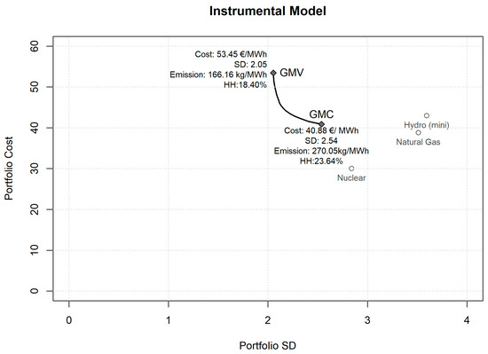
Figure 1.
Instrumental model’s efficient frontier.
Figure 2 represents the participation shares of the different technologies in the efficient frontier portfolios of the instrumental model. As we can see, the GMV portfolio, the one on the left side of the figure, shows a higher diversification—its Herfindahl–Hirschman index is 18.40%, less than the GMC portfolio with a Herfindahl–Hirschman index of 23.64%, which is considered good for energy security.
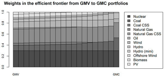
Figure 2.
Technology participation in the instrumental mode.
Moreover, the nuclear, the small hydro, as well as the offshore wind technologies participate in the GMV portfolio at their maxima. On the other hand, in the GMC portfolio, the nuclear, the coal, the natural gas, the hydro, the small hydro, and the offshore wind technologies play a part at their maxima. Therefore, nuclear, small hydro, and offshore wind are regarded as highly efficient technologies in terms of cost and risk by the model.
The next step will be to classify the different generation technologies into two different subsets: one for the pollutant technologies—coal, coal with CCS, natural gas, natural gas with CCS, oil, and biomass—and another one for the non-pollutant technologies—nuclear, wind, offshore wind, hydro, small hydro, and PV. For the first subset, we are going to set out a model quite similar to the instrumental one just exposed. For the second subset, we will consider an emission-risk model instead of a cost-risk model.
2.3.2. The Non-Pollutant Technology Efficient Frontier
Using the same data shown in Table 1 and Table 2 but considering only those non-pollutant technologies, we will adapt the technological and environmental constraints of the instrumental model to obtain the constraints pertinent to this non-pollutant technologies model. To adapt the technological and environmental constraints of the instrumental model to the non-pollutant technologies, we decided to work on the basis of the non-pollutant technology’s participation shares in the efficient frontier calculated in the previous section. Briefly, we raised the participation share of every non-pollutant technology relative to the total non-pollutant technologies participation shares in every efficient portfolio and took the maximum by technology, resulting in the limits presented in Table 4, where the column “Maximum Weight” refers to the maximum weight reached in the efficient frontier of the previous model and the column “Maximum Participation” refers to this maximum weight considering only the non-pollutant technologies.
Table 4.
Non-pollutant technological and environmental limits. Source: Authors’ own work, based on data collected from DeLlano et al. (2015) [14].
Thus, the non-pollutant model is presented in Equation (4); keep in mind that the cost restriction is used to calculate the efficient frontier as described in the previous section.
Solving this model, we obtain the efficient frontier shown in Figure 3. Note that the dashed grey line shown is the instrumental model efficient frontier from the previous section. Comparing both efficient frontiers, the one from the instrumental model and the one from the non-pollutant technology model, we can observe that the instrumental model shows higher costs but lower risks—as its efficient frontier is displaced upward and toward the left.
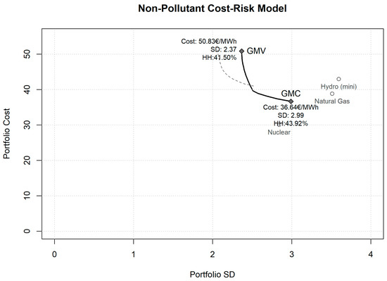
Figure 3.
Non-pollutant technology model’s efficient frontier.
Analysing the weights in the GMV and GMC portfolios, we see that nuclear and small hydro participate again at their maxima in both portfolios. In particular, in the GMV portfolio, the offshore wind also participates at its maximum, while in the GMC portfolio, it is the hydro technology that also enters at its maximum.
Not surprisingly, the Herfindahl–Hirschman index is worse than in the instrumental model, the non-pollutant technology model has fewer technologies, and again, the GMV portfolio is more diversified than the GMC portfolio.
2.3.3. The Emission-Risk Pollutant Technology Efficient Frontier
We will replace our cost-risk orientation with an emission-risk orientation in this second stage of the model presented in this work. As stated, we have no emission data, apart from the emission average shown in Table 1, and hence, we use the CO2 cost standard deviation as a proxy for the emission standard deviation. According to this information, we simulated 100,000 normal distributed values to calculate the variance-covariance matrix shown in Table 5.
Table 5.
Emission variance-covariance matrix.
The pollutant technology emission-risk model presented in this section is highly similar to the instrumental model except for the following two aspects. Firstly, we are not using costs in the current model but emission factors for the six pollutant technologies—coal, coal with CCS, natural gas, natural gas with CCS, oil, and biomass. Secondly, we will show five different adaptations of the current model, four of them without constraints other than the model technical constraints. In the other model adaptation, we include technological constraints for the pollutant technologies. The limits of these constraints were built in a quite similar manner as that for the non-pollutant technology model presented in Section 2.3.2., i.e., raising every pollutant technology participation in the instrumental model efficient frontier portfolios relative to the total pollutant technologies in those portfolios and getting the maximum participation as the limit. A problem arises as the oil technology is not participating in any of the calculated portfolios. To fix it, its technological and environmental limits in the instrumental model are relatively raised to the limits set for the pollutant technologies.
2.3.4. Model Adaptation with All the Non-Pollutant Technologies
For the six pollutant technologies, we solved the model presented in Equation (5), in which is the emission factor of the portfolio and is the emission vector of which the elements can be found in Table 1:
In this model we substituted the cost constraint for an emission constraint as we are working with emission-risk pairs instead of cost-risk pairs.
The results of this model are trivial because, in the GMV portfolio, 99.88% of the power generation is assigned to biomass and, in the global minimum emission portfolio (GME), biomass captures 100% of the power generation. The efficient frontier is hence insignificant and practically indistinguishable from a portfolio with 100% biomass generation. These results were expected as biomass shows a very low level of CO2 emission as compared to the rest of pollutant technologies and a negligible level of risk. In fact, this result is completely in line with the optimization features of the model.
A single-technology generation portfolio, or a generation portfolio in which one single technology is responsible for such a big part of the power generation, is quite far from being an acceptable solution from the point of view of energy planning. Next, we develop some model adaptations to deal with this circumstance.
2.3.5. Model Adaptations without CCS Technologies and without Biomass Technology
The first adaptation is similar to the previous one, but CCS technologies, both coal and natural gas, are removed to prevent the possibility of these technologies not being able to reach a feasible commercial availability. The results are therefore similar: biomass hoards 99.99% of the generation in the GMV portfolio and 100% of the generation in the GME portfolio because of the reasons exposed above.
In the second model adaptation, biomass technology is removed from the model. The results offer a bit more information than in the previous models. Figure 4 shows the weights of the five considered technologies from the GMV portfolio—first column on the left—to the GME portfolio—last column. The GMV portfolio allows entry of every technology to the generation mix although natural gas with CCS takes the lion’s share—the Herfindahl–Hirschman index is 65.96% for this portfolio. As we move from the GMV portfolio to the GME portfolio, it is clear that natural gas with CCS is increasing its participation share until it reaches 100% in the GME portfolio.
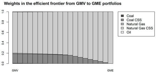
Figure 4.
Non-pollutant technology model’s efficient frontier.
The third model adaptation shows what happens if neither CCS technologies nor biomass are available to generate power. Again, natural gas, in this case without CCS, is the dominant generation technology. Surprisingly, oil takes the second place. This is due to the correlations between oil and the other two technologies in this model adaptation. Figure 5 shows the weights of the considered technologies in the efficient frontier portfolios—from the GMV portfolio on the left to the GME portfolio on the right.
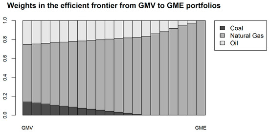
Figure 5.
Model adaptation without both carbon capture and storage (CCS) and biomass technologies.
2.3.6. Model Adaptation with Technological Constraints
In this model adaptation, the problem to solve will be the one presented in Equation (6).
As stated, the limits were taken from the instrumental model efficient frontier participation shares of the pollutant technologies, except for the oil technology limit that was taken from the instrumental model technological limits of the pollutant technologies.
Solving this model adaptation, the results shown in Figure 6 are achieved. As expected, in light of the precedent results, biomass is participating at its maximum in every efficient frontier portfolio. When they participate in the less risky portfolios, coal, natural gas, and oil have participation shares around 1%. In the GME portfolio, natural gas with CCS participates at the maximum set for natural gas with and without CCS. The little variation in participation shares due to the imposed constraints will give us a short efficient frontier.
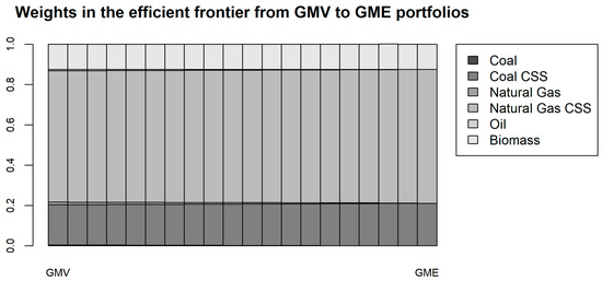
Figure 6.
Model adaptation with technological constraints.
3. Results
In this section, we present our main results related to cross-drawing the instrumental model and the pollutant-technology model. Additionally, we will discuss how this model can help policy makers make their decisions.
3.1. Cross-Drawing the Cost-Risk and Emission-Risk Models and Selecting an Adequate Combination of Non-Pollutant and Pollutant Technologies
So far, we have one instrumental model that includes all the technologies and constraints, a non-pollutant efficient frontier that shows higher risk but lower cost than the instrumental efficient frontier, and a set of several adaptations of a model with pollutant-technologies. Figure 7 represents some of the efficient frontiers calculated in an emission-risk coordinate axis. Specifically, we depict the instrumental model numbered with 0 and with a dot-dash line, the model adaptations without biomass numbered as 2.c, those without biomass and CSS technologies numbered as 2.d, and those with all the pollutant technologies and with technological constraints numbered as 2.e. It is important to note that the first two adaptations were practically 100% biomass participated, and for this reason, we are not showing them in the graph—they would be located practically where the biomass technology is drawn.
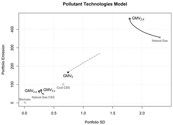
Figure 7.
Efficient frontiers in an emission-risk plane.
Regarding the pollutant models, the traditional pollutant technologies—coal, natural gas, and oil—show higher levels of emission and risk; model 2.d efficient frontier appears on the top right side of the figure. If CCS technologies are included, both the emission and the risk levels are drastically reduced; see model 2.c in the figure. In fact, models 2.a and 2.b would be represented over the biomass point in Figure 6. Moreover, the technological constraints are able to lower even more the risk, keeping a similar level of emission—model 2.e.
By representing in the same emission-risk plane our instrumental model, model 0, it is worth comparing it with the pollutant models—the non-pollutant model would be drawn on the coordinate origin. The instrumental model shows a higher level of emission and risk, in terms of emission, than those models allowing biomass and CCS technologies because coal and natural gas participate largely in it, as shown in Figure 2. When approaching the GMC portfolio, these technologies reach their technological limit and, actually, they participate at their maxima in the GMC portfolio.
The efficient frontier of our models is drawn in a cost-risk coordinate axis in Figure 8. Both the instrumental model, model 0, and the pollutant models, models 2.e and 2.d, present smaller levels of risk with similar or lower levels of cost. As stated, pollutant models with biomass, models 2.a and 2.b, would be drawn on the point corresponding to biomass technology that is far out of the graph’s limits with a cost variance of 162.84 (standard deviation: 12.76 €/MWh) and with a cost of 96.62 €/MWh.
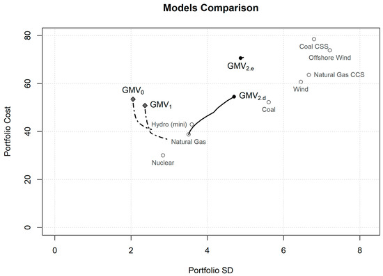
Figure 8.
Efficient frontiers in a cost-risk plane.
3.2. The CML-Analogous Area
So far, we have a pollutant-technology efficient frontier from an emission-risk perspective and a point of the emission-risk coordinate axis origin representing all the non-pollutant efficient portfolios. A policy maker could compile a portfolio from the pollutant-technology efficient frontier with the point in the origin to determine a power-generation portfolio with the whole set of technologies. Therefore, it is possible to set the best portfolio given a desired emission factor or a risk limit.
The limits of the pollutant-technology efficient frontier are the GMV and the GME portfolios. The efficient frontier itself connects them together. Combinations of either the GMV or the GME portfolio with any of the non-pollutant efficient portfolios in the origin will fall inside an area delimited by these three portfolios: the GMV portfolio, the GME portfolio, and the non-pollutant efficient portfolio chosen. In Figure 9, this area is the shaded area below and to the left of the pollutant-technology efficient frontier.
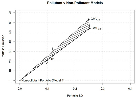
Figure 9.
A Capital Market Line (CML)-Analogous analysis.
Being under the efficient frontier reflects that any point inside that area shows a lower emission factor than the point on the frontier with the same level of risk. This was expected as we are combining a pollutant portfolio with a non-pollutant one. On the other hand, the fact of being to the left of the pollutant efficient frontier indicates that the risk is lower for any emission factor considered. A portfolio inside the CML-analogous area (CML-A) is then more efficient than a portfolio in the efficient frontier with the same emission factor or level of risk.
Focusing on the CML-A, the problem is to determine the best portfolio for a given emission factor or for a given level of risk. It is easy to conclude that the answer must be found on the CML-A borders. Indeed, when determining the best portfolio in the CML-A for a given level of risk, the solution must be that one located on the segment joining the coordinate axis origin and the GME portfolio that shows that level of risk. Likewise, if we want to determine the best portfolio in the CML-A for a given emission factor, we must find it on the intersection of the segment joining the GMV portfolio with the coordinate axis origin and the line representing the desired emission factor. In the next section, we present a brief example of these ideas.
4. Discussion
In this section, there is a brief explanation of how a policy maker could employ this model to design power-generation portfolios. In Figure 9, we draw one of our pollutant efficient frontiers, specifically model 2.e, with all the pollutant technologies and with technological constraints in an emission-risk coordinate axis. In this graph, the non-pollutant model portfolios will be all of them on the coordinate origin; they have no emission and, consequently, no emission risk.
A policy maker can choose any combination: any linear combination between any portfolio on the pollutant efficient frontier and on the non-pollutant efficient frontier which, from an emission point of view, lays on the coordinate origin. In Figure 9, the shaded area delimited by the coordinate origin and the pollutant efficient frontier of model 2.e represents these combinations. We can see that the area allows the policy maker to lower the risk for a given level of emission or the emission for a given level of risk. For instance, given the emission and risk values for GMV and GME portfolios of model 2.e shown in Table 6, it is easy to calculate the portfolio proportions needed to reach an emission risk of 0.10 kg/MWh. Obviously, the policy maker will prefer the lowest emission possible for that level of risk and so they will choose the pollutant GME portfolio for the combination, resulting in point A in Figure 9. Point A can be reached by combining the pollutant GME portfolio and the non-pollutant portfolio in a proportion of 39.39–60.61%. Also, the policy maker could want to set the emission of the resultant portfolio, say, at 30 kg/MWh. In this case, they would like to reach a minimum risk combination for that level of emission. For this reason, they will want to combine the pollutant GMV portfolio with the non-pollutant portfolio, resulting in point B, which corresponds to a 47.44–52.56% proportion of pollutant GMV and non-pollutant portfolios.
Table 6.
Emission and risk of the global minimum variance (GMV) and global minimum emission (GME) portfolios of model 2.e.
In the last example, it is easy to see that the combination B’ with a 46.75% GME portfolio and a 53.25% non-pollutant portfolio has the same risk value as combination B but with a lower emission of 25.15 kg/MWh. It does not seem reasonable to lose the opportunity to lower emissions without increasing the risk. This is why the lower segment of the shaded area is more efficient in the sense used in this work than the rest of the points in the area when the aim is to adapt the generation portfolio to a predetermined risk. This insight is similar to the financial CML, but in our case and due to the convexity of the efficient frontier, instead of having a tangency or market portfolio, we propose to use the corresponding GME portfolio instead.
5. Conclusions
Throughout the present work, we proved that it is possible to separate the generation technologies into two different sets and to proceed to a double optimization of the generation mix. When we compare the non-pollutant-technology efficient frontier with the efficient frontier of the instrumental model, we are able to generate at a lower cost but at a higher risk using only non-pollutant technologies (nuclear, wind, offshore wind, hydro, small hydro, and PV).
When analysing the sharing weights in the non-pollutant efficient frontier, nuclear energy, defending its position as a base-load generation technology, and small hydro participate at their maxima in both the minimum-risk GMV and the minimum-cost GMC portfolios:
- Nuclear and small hydro are preferential technologies that act as if it intends to obtain the minimum cost or to get the minimum risk of the portfolio.
- In a complementary way, offshore wind technology participates at its maximum share if the minimum risk is searched, while large hydro technology is the third technology to enter its maximum in the minimum cost portfolio.
Replacing the cost-risk perspective with emission-risk perspective pollutant technologies allows to highlight the important role of biomass and CCS technologies in an efficient portfolio. Their commercial development is crucial in order to achieve low-carbon emission portfolios.
Oil generation is not included in the power-generation mix in the instrumental model, highlighting its excessive cost and risk. In the emission-risk models, it is only considered when we take out the biomass or when we set upper limits to the participation shares of the technologies. These limits cause the preferred technologies to participate at their maxima in almost every efficient portfolio.
Solar PV generation takes part only in the efficient portfolios close to the GMV portfolio. Its participation is needed in order to achieve a highly diversified and lower risk portfolio.
The cross-drawing approach proposed between the pollutant and non-pollutant efficient frontiers calculated in both cost-risk and emission-risk coordinate axes leads to relevant conclusions:
- A pollutant-only generation mix shows a higher cost than a complete generation technology portfolio and even in relation to the non-pollutant-only efficient frontier.
- A highly diversified portfolio makes it possible to achieve the lowest risk (instrumental model).
- Renewable energy sources are needed to reduce portfolio cost and risk.
- Pollutant-generation-efficient frontiers show a higher risk mainly because of the fuel cost risk.
Finally, drawing an analogy with the CML from CAPM, we presented the CML-A area that could helpful a policy maker design the long-term generation mix in a decarbonisation scenario.
Author Contributions
The Contributor Roles Taxonomy (CRediT) of this work is as follows: conceptualization, P.M.-F., F.d.-P. and I.S.; methodology: P.M.-F., F.d.-P. and A.C.-S.; software, P.M.-F.; validation, F.d.-P.; formal analysis, P.M.-F., F.d.-P. and A.C.-S.; investigation: F.d.-P.; resources, F.d.-P. and I.S.; data curation, P.M.-F. and F.d.-P.; writing – original draft preparation, P.M.-F. and F.d.-P.; writing – review and editing, P.M.-F.; visualization, P.M.-F. and F.d.-P.; supervision, A.C.-S. and I.S.; project administration, P.M.-F. and F.d.-P.; funding acquisition: A.C.-S.
Funding
This research received no external funding.
Conflicts of Interest
The authors declare no conflict of interest.
References
- Cormio, C.; Dicorato, M.; Minoia, A.; Trovato, M. A regional energy planning methodology including renewable energy sources and environmental constraints. Renew. Sustain. Energy Rev. 2003, 7, 99–130. [Google Scholar] [CrossRef]
- Huang, Y.-H.; Wu, J.-H.; Hsu, Y.-J. Two-stage stochastic programming model for the regional-scale electricity planning under demand uncertainty. Energy 2016, 116, 1145–1157. [Google Scholar] [CrossRef]
- Liu, Y.; He, L.; Shen, J. Optimization-based provincial hybrid renewable and non-renewable energy planning—A case study of Shanxi, China. Energy 2017, 128, 839–856. [Google Scholar] [CrossRef]
- Nie, S.; Li, Y.P.; Liu, J.; Huang, C.Z. Risk management of energy system for identifying optimal power mix with financial-cost minimization and environmental-impact mitigation under uncertainty. Energy Econ. 2017, 61, 313–329. [Google Scholar] [CrossRef]
- Kim, S.; Koo, J.; Lee, C.J.; Yoon, E.S. Optimization of Korean energy planning for sustainability considering uncertainties in learning rates and external factors. Energy 2012, 44, 126–134. [Google Scholar] [CrossRef]
- Codina Gironès, V.; Moret, S.; Maréchal, F.; Favrat, D. Strategic energy planning for large-scale energy systems: A modelling framework to aid decision-making. Energy 2015, 90, 173–186. [Google Scholar] [CrossRef]
- Sáfián, F. Modelling the Hungarian energy system—The first step towards sustainable energy planning. Energy 2014, 69, 58–66. [Google Scholar] [CrossRef]
- Gómez, A.; Dopazo, C.; Fueyo, N. The “cost of not doing” energy planning: The Spanish energy bubble. Energy 2016, 101, 434–446. [Google Scholar] [CrossRef]
- Allan, G.; Eromenko, I.; McGregor, P.; Swales, K. The regional electricity generation mix in Scotland: A portfolio selection approach incorporating marine technologies. Energy Policy 2011, 39, 6–22. [Google Scholar] [CrossRef]
- Arnesano, M.; Carlucci, A.P.; Laforgia, D. Extension of portfolio theory application to energy planning problem—The Italian case. Energy 2012, 39, 112–124. [Google Scholar] [CrossRef]
- Awerbuch, S. Portfolio-Based Electricity Generation Planning: Implications for Renewables and Energy Security. Mitig. Adapt. Strateg. Glob. Chang. 2004, 11, 693–710. [Google Scholar] [CrossRef]
- Awerbuch, S.; Jansen, J.C.; Beurskens, L. The Role of Wind Generation in Enhancing Scotland’s Energy Diversity and Security: A Mean-Variance Portfolio Optimization of Scotland’s Generating Mix. In Analytical Methods for Energy Diversity & Security; Elsevier: Amsterdam, The Netherlands, 2008; pp. 139–150. [Google Scholar]
- Bhattacharya, A.; Kojima, S. Power sector investment risk and renewable energy: A Japanese case study using portfolio risk optimization method. Energy Policy 2012, 40, 69–80. [Google Scholar] [CrossRef]
- Dellano-Paz, F.; Calvo-Silvosa, A.; Iglesias Antelo, S.; Soares, I. The European low-carbon mix for 2030: The role of renewable energy sources in an environmentally and socially efficient approach. Renew. Sustain. Energy Rev. 2015, 48, 49–61. [Google Scholar] [CrossRef]
- Delarue, E.; De Jonghe, C.; Belmans, R.; D’haeseleer, W. Applying portfolio theory to the electricity sector: Energy versus power. Energy Econ. 2011, 33, 12–23. [Google Scholar] [CrossRef]
- Dellano-Paz, F.; Calvo-Silvosa, A.; Antelo, S.I.; Soares, I. Energy planning and modern portfolio theory: A review. Renew. Sustain. Energy Rev. 2017, 77, 636–651. [Google Scholar] [CrossRef]
- Kumar, D.; Mohanta, D.K.; Reddy, M.J.B. Intelligent optimization of renewable resource mixes incorporating the effect of fuel risk, fuel cost and CO2 emission. Front. Energy 2015, 9, 91–105. [Google Scholar] [CrossRef]
- Gao, C.; Sun, M.; Shen, B.; Li, R.; Tian, L. Optimization of China’s energy structure based on portfolio theory. Energy 2014, 77, 890–897. [Google Scholar] [CrossRef]
- Gökgöz, F.; Atmaca, M.E. Financial optimization in the Turkish electricity market: Markowitz’s mean-variance approach. Renew. Sustain. Energy Rev. 2012, 16, 357–368. [Google Scholar] [CrossRef]
- Lucheroni, C.; Mari, C. CO2 volatility impact on energy portfolio choice: A fully stochastic LCOE theory analysis. Appl. Energy 2017, 190, 278–290. [Google Scholar] [CrossRef]
- Roques, F.; Hiroux, C.; Saguan, M. Optimal wind power deployment in Europe—A portfolio approach. Energy Policy 2010, 38, 3245–3256. [Google Scholar] [CrossRef]
- Zhu, L.; Fan, Y. Optimization of China’s generating portfolio and policy implications based on portfolio theory. Energy 2010, 35, 1391–1402. [Google Scholar] [CrossRef]
- Chen, Y.; He, L.; Guan, Y.; Lu, H.; Li, J. Life cycle assessment of greenhouse gas emissions and water-energy optimization for shale gas supply chain planning based on multi-level approach: Case study in Barnett, Marcellus, Fayetteville, and Haynesville shales. Energy Convers. Manag. 2017, 134, 382–398. [Google Scholar] [CrossRef]
- Shaban Boloukat, M.H.; Akbari Foroud, A. Stochastic-based resource expansion planning for a grid-connected microgrid using interval linear programming. Energy 2016, 113, 776–787. [Google Scholar] [CrossRef]
- Falsafi, H.; Zakariazadeh, A.; Jadid, S. The role of demand response in single and multi-objective wind-thermal generation scheduling: A stochastic programming. Energy 2014, 64, 853–867. [Google Scholar] [CrossRef]
- Koltsaklis, N.E.; Liu, P.; Georgiadis, M.C. An integrated stochastic multi-regional long-term energy planning model incorporating autonomous power systems and demand response. Energy 2015, 82, 865–888. [Google Scholar] [CrossRef]
- Tajeddini, M.A.; Rahimi-Kian, A.; Soroudi, A. Risk averse optimal operation of a virtual power plant using two stage stochastic programming. Energy 2014, 73, 958–967. [Google Scholar] [CrossRef]
- Stempien, J.P.; Chan, S.H. Addressing energy trilemma via the modified Markowitz Mean-Variance Portfolio Optimization theory. Appl. Energy 2017, 202, 228–237. [Google Scholar] [CrossRef]
- Jansen, J.C.; Beurskens, L.W.M.; Van Tilburg, X. Application of Portfolio Analysis to the Dutch Generating Mix; Reference case and two renewables cases, Year 2030, SE and GE scenario (No. ECN-C-05-100); Energy research Centre of the Netherlands ECN: Sint Maartensvlotbrug, The Netherlands, 2006. [Google Scholar]
- Dellano-Paz, F.; Martínez Fernandez, P.; Soares, I. Addressing 2030 EU policy framework for energy and climate: Cost, risk and energy security issues. Energy 2016, 115, 1347–1360. [Google Scholar] [CrossRef]
- Hickey, E.A.; Lon Carlson, J.; Loomis, D. Issues in the determination of the optimal portfolio of electricity supply options. Energy Policy 2010, 38, 2198–2207. [Google Scholar] [CrossRef]
- Jano-Ito, M.A.; Crawford-Brown, D. Investment decisions considering economic, environmental and social factors: An actors’ perspective for the electricity sector of Mexico. Energy 2017, 121, 92–106. [Google Scholar] [CrossRef]
- Chuang, M.C.; Ma, H.W. Energy security and improvements in the function of diversity indices—Taiwan energy supply structure case study. Renew. Sustain. Energy Rev. 2013, 24, 9–20. [Google Scholar] [CrossRef]
- Böhringer, C.; Bortolamedi, M. Sense and no(n)-sense of energy security indicators. Ecol. Econ. 2015, 119, 359–371. [Google Scholar] [CrossRef][Green Version]
- Muñoz, B.; García-Verdugo, J.; San-Martín, E. Quantifying the geopolitical dimension of energy risks: A tool for energy modelling and planning. Energy 2015, 82, 479–500. [Google Scholar] [CrossRef]
- Apergis, N.; Payne, J.E.; Menyah, K.; Wolde-Rufael, Y. On the causal dynamics between emissions, nuclear energy, renewable energy, and economic growth. Ecol. Econ. 2010, 69, 2255–2260. [Google Scholar] [CrossRef]
- Johansson, B. Security aspects of future renewable energy systems–A short overview. Energy 2013, 61, 598–605. [Google Scholar] [CrossRef]
- Labandeira, X. Sistema Energético Y Cambio Climático: Prospectiva Tecnológica y Regulatoria (No. 02); Working Papers 2012; Economics for Energy (eforenergy.org): Vigo, Spain, 2012. [Google Scholar]
- Labandeira, X.; Linares, P.; Würzburg, K. Energías Renovables Y Cambio Climático (No. 06); Working Papers 2012; Economics for Energy (eforenergy.org): Vigo, Spain.
- Akter, S.; Kompas, T.; Ward, M.B. Application of portfolio theory to asset-based biosecurity decision analysis. Ecol. Econ. 2015, 117, 73–85. [Google Scholar] [CrossRef]
- Tolmasquim, M.T.; Seroa da Motta, R.; La Rovere, E.L.; Barata MM de, L.; Monteiro, A.G. Environmental valuation for long-term strategic planning—The case of the Brazilian power sector. Ecol. Econ. 2001, 37, 39–51. [Google Scholar] [CrossRef]
- Urhammer, E. Celestial bodies and satellites—Energy issues, models, and imaginaries in Denmark since 1973. Ecol. Econ. 2017, 131, 425–433. [Google Scholar] [CrossRef]
- Bennink, D.; Rooijers, F.; Croezen, H.; de Jong, F.; Markowska, A. VME Energy Transition Strategy: External Costs and Benefits of Electricity Generation, Transition; CE Delft: Delft, The Netherlands, 2010. [Google Scholar]
- Eyre, N. External costs. What do they mean for energy policy? Energy Policy 1997, 25, 85–95. [Google Scholar] [CrossRef]
- Söderholm, P.; Sundqvist, T. Pricing environmental externalities in the power sector: Ethical limits and implications for social choice. Ecol. Econ. 2003, 46, 333–350. [Google Scholar] [CrossRef]
- Awerbuch, S.; Yang, S. Efficient Electricity Generating Portfolios for Europe: Maximising Energy Security and Climate Change Mitigation; EIB Papers; EIB: Kirchberg, Luxembourg, 2007. [Google Scholar]
- Cucchiella, F.; D’Adamo, I.; Gastaldi, M. Optimizing plant size in the planning of renewable energy portfolios. Lett. Spat. Resour. Sci. 2016, 9, 169–187. [Google Scholar] [CrossRef]
- Lynch, M.Á.; Shortt, A.; Tol, R.S.J.; O’Malley, M.J. Risk–return incentives in liberalised electricity markets. Energy Econ. 2013, 40, 598–608. [Google Scholar] [CrossRef]
- Antimiani, A.; Costantini, V.; Kuik, O.; Paglialunga, E. Mitigation of adverse effects on competitiveness and leakage of unilateral EU climate policy: An assessment of policy instruments. Ecol. Econ. 2016, 128, 246–259. [Google Scholar] [CrossRef]
- Monjon, S.; Quirion, P. Addressing leakage in the EU ETS: Border adjustment or output-based allocation? Ecol. Econ. 2011, 70, 1957–1971. [Google Scholar] [CrossRef]
- Oberndorfer, U. EU Emission Allowances and the stock market: Evidence from the electricity industry. Ecol. Econ. 2009, 68, 1116–1126. [Google Scholar] [CrossRef]
- Rogge, K.S.; Schneider, M.; Hoffmann, V.H. The innovation impact of the EU Emission Trading System—Findings of company case studies in the German power sector. Ecol. Econ. 2011, 70, 513–523. [Google Scholar] [CrossRef]
- Dincer, I. Renewable energy and sustainable development: A crucial review. Renew. Sustain. Energy Rev. 2000, 4, 157–175. [Google Scholar] [CrossRef]
- Escribano Francés, G.; Marín-Quemada, J.M.; San Martín González, E. RES and risk: Renewable energy’s contribution to energy security. A portfolio-based approach. Renew. Sustain. Energy Rev. 2013, 26, 549–559. [Google Scholar] [CrossRef]
- Panwar, N.L.; Kaushik, S.C.; Kothari, S. Role of renewable energy sources in environmental protection: A review. Renew. Sustain. Energy Rev. 2011, 15, 1513–1524. [Google Scholar] [CrossRef]
- Martinez-Fernandez, P.; deLlano-Paz, F.; Calvo-Silvosa, A.; Soares, I. Pollutant versus non-pollutant generation technologies: A CML-analogous analysis. Environ. Dev. Sustain. 2018, 20 (Suppl. 1), 199–212. [Google Scholar] [CrossRef]
- Jaffe, A.B.; Newell, R.G.; Stavins, R.N. A tale of two market failures: Technology and environmental policy. Ecol. Econ. 2005, 54, 164–174. [Google Scholar] [CrossRef]
- Markowitz, H. Portfolio Selection. J. Financ. 1952, 7, 77–91. [Google Scholar] [CrossRef]
- Sharpe, W.F. A Simplified Model for Portfolio Analysis. Manage. Sci. 1963, 9, 277–293. [Google Scholar] [CrossRef]
- Sharpe, W.F. Capital Asset Prices: A Theory of Market Equilibrium under Conditions of Risk. J. Financ. 1964, 19, 425. [Google Scholar] [CrossRef]
- Min Liu Wu, F.F.; Yixin, N.I. A survey on risk management in electricity markets. In Proceedings of the 2006 IEEE Power Engineering Society General Meeting, Montreal, QC, Canada, 18–22 June 2006; IEEE: Piscataway, NJ, USA, 2006; p. 6. [Google Scholar] [CrossRef]
- Westner, G.; Madlener, R. The benefit of regional diversification of cogeneration investments in Europe: A mean-variance portfolio analysis. Energy Policy 2010, 38, 7911–7920. [Google Scholar] [CrossRef]
- Chae, J.; Joo, S.-K. Demand Response Resource Allocation Method Using Mean-Variance Portfolio Theory for Load Aggregators in the Korean Demand Response Market. Energies 2017, 10, 879. [Google Scholar] [CrossRef]
- Yemshanov, D.; Koch, F.H.; Lu, B.; Lyons, D.B.; Prestemon, J.P.; Scarr, T.; Koehler, K. There is no silver bullet: The value of diversification in planning invasive species surveillance. Ecol. Econ. 2014, 104, 61–72. [Google Scholar] [CrossRef]
- Stirling, A. Diversity and ignorance in electricity supply investment: Addressing the solution rather than the problem. Energy Policy 1994, 22, 195–216. [Google Scholar] [CrossRef]
- Stirling, A. On the Economics and Analysis of Diversity; Science and Technology Policy Research (SPRU) Electronic Working Paper Series; Paper No. 28; University of Sussex: Brighton, UK, 1998. [Google Scholar]
- Kruyt, B.; van Vuuren, D.P.; de Vries, H.J.M.; Groenenberg, H. Indicators for energy security. Energy Policy 2009, 37, 2166–2181. [Google Scholar] [CrossRef]
- Charwand, M.; Gitizadeh, M.; Siano, P. A new active portfolio risk management for an electricity retailer based on a drawdown risk preference. Energy 2017, 118, 387–398. [Google Scholar] [CrossRef]
- Karandikar, R.G.; Khaparde, S.A.; Kulkarni, S.V. Quantifying price risk of electricity retailer based on CAPM and RAROC methodology. Int. J. Electr. Power Energy Syst. 2007, 29, 803–809. [Google Scholar] [CrossRef]
- Rohlfs, W.; Madlener, R. Assessment of clean-coal strategies: The questionable merits of carbon capture-readiness. Energy 2013, 52, 27–36. [Google Scholar] [CrossRef]
- Cheng, C.; Wang, Z.; Liu, M.; Chen, Q.; Gbatu, A.P.; Ren, X. Defer option valuation and optimal investment timing of solar photovoltaic projects under different electricity market systems and support schemes. Energy 2017, 127, 594–610. [Google Scholar] [CrossRef]
- Copiello, S.; Gabrielli, L.; Bonifaci, P. Evaluation of energy retrofit in buildings under conditions of uncertainty: The prominence of the discount rate. Energy 2017, 137, 104–117. [Google Scholar] [CrossRef]
- Shimbar, A.; Ebrahimi, S.B. The application of DNPV to unlock foreign direct investment in waste-to-energy in developing countries. Energy 2017, 132, 186–193. [Google Scholar] [CrossRef]
- Zhang, G.; Du, Z. Co-movements among the stock prices of new energy, high-technology and fossil fuel companies in China. Energy 2017, 135, 249–256. [Google Scholar] [CrossRef]
- Broadstock, D.C.; Filis, G. Oil price shocks and stock market returns: New evidence from the United States and China. J. Int. Financ. Mark. Inst. Money 2014, 33, 417–433. [Google Scholar] [CrossRef]
- Schaeffer, R.; Borba, B.S.M.C.; Rathmann, R.; Szklo, A.; Castelo Branco, D.A. Dow Jones sustainability index transmission to oil stock market returns: A GARCH approach. Energy 2012, 45, 933–943. [Google Scholar] [CrossRef]
- De-Llano, F.; Iglesias, S.; Calvo, A.; Soares, I. The technological and environmental efficiency of the EU-27 power mix: An evaluation based on MPT. Energy 2014, 69, 67–81. [Google Scholar] [CrossRef]


© 2019 by the authors. Licensee MDPI, Basel, Switzerland. This article is an open access article distributed under the terms and conditions of the Creative Commons Attribution (CC BY) license (http://creativecommons.org/licenses/by/4.0/).