Abstract
The battery state of charge (SOC) and state of power (SOP) are two essential parameters in the battery management system. For power lithium-ion batteries, temperature variation and the hysteresis effect are two of the main negative contributions to the accuracy of model-based SOC and SOP estimation. Thereby, a reliable circuit model is established herein to accurately estimate the working state of batteries. Considering the effect that temperature and hysteresis have on the electrical system, a unique fully-coupled temperature–hysteresis model is proposed to describe the interrelationship among capacity, hysteresis voltage, and temperature comprehensively. The key parameters of the proposed model are identified by experiments operated on lithium-ion batteries under varying ambient temperatures. Then we build a multi-state joint estimator to calculate the SOC and SOP on the basis of the temperature–hysteresis model. The effectiveness of the advanced model is verified by experiments at different temperatures. Moreover, the proposed joint estimator is verified by the improved dynamic stress test. The experimental results indicate that the proposed estimator making use of the temperature–hysteresis model can estimate SOC and SOP accurately and robustly. Our results also prove invaluable in terms of the construction of a flexible battery management system for applications in the actual industrial field.
1. Introduction
With the rapid development of the automobile industry, the energy crisis and environmental pollution have accelerated the research and application of electric vehicles (EV) [1]. Power battery is the heart of EV, and its safety and reliability should be ensured [2]. An accurate estimation of the state of charge (SOC) achieves the remaining power of the battery accurately. Furthermore, the SOC is the key factor for the battery management system (BMS) and the basis for the EVs’ power allocation strategies [3,4,5]. The state of power (SOP) is an index reflecting the instantaneous power performance of the battery. It can be used to judge whether the EV meets the requirements of acceleration, regenerative braking, and gradeability [6,7,8]. Compared with the SOC and the State of Health (SOH), the SOP can more directly reflect the exchange of energy between the battery system and the external system [9]. The battery’s SOP is constantly changing under the influence of factors such as temperature, internal resistance, SOC, etc. Thus, as to ensure the safety of the battery, the exact monitoring and accurate prediction for the SOP are necessary [10]. The researches on battery’s SOC and SOP estimation algorithm based on modeling is able to provide a powerful basis for the optimization of EVs’ BMS.
In order to ensure the effectiveness of battery state estimation, it is necessary to establish an accurate battery model. Because the working process of the battery is composed of a series of complex electrochemical processes, researchers model the battery from various perspectives. The introduction of an equivalent-circuit model (ECM) makes the implementation of the battery model less difficult. It works by using electrical components to characterize the key features of the battery during charging and discharging [11]. Compared with the electrochemical Model, ECM is able to operate with fewer inputs but high regression performance. The parameters in the model can be identified by offline or online methods [12]. Compared with the model based on machine learning, ECM has the advantages of a shorter calculation time, faster response speed, and parameters with definite physical meanings. In addition, the model can be easily integrated into the BMS and power control system of the electric vehicle. Therefore, ECM is a generic model for broad usage in practice. [13]. In the previous researches, the first, second, and higher order resistor-capacitance (RC) models were used to simulate the non-linear characteristics of batteries for ECM [14,15]. The higher order RC equivalent circuit model reflects the dynamic performance of batteries more comprehensively. Furthermore, multi-time scale filters are used to identify the parameters of the battery model and predict the battery operating state [16]. However, the higher order of the model results in a more complicated calculation process. As a result, considering the large computational complexity of high-order model and the large error of the first-order model, most scholars choose the second-order or third-order RC model as the research basis of state estimation, taking the calculation accuracy and real-time performance into account [17]. Meanwhile, for Lithium-ion batteries, the hysteretic characteristics of open-circuit voltage and charging state are very necessary to be characterized when ECM is selected as the battery model [18]. The second-order RC ECM considering voltage hysteretic characteristics is simulated. The simulation results show that the accuracy of the model is higher than that of the second-order RC model alone, and it can track the actual voltage well [19]. Although the hysteresis characteristics are introduced into the above model, the influence of temperature on battery modeling is not considered at all, thus the accuracy of that battery model is still insufficient.
The battery SOP is in effect affected by a series of key parameters, including battery capacity, internal resistance, SOC, and temperature [20]. Because SOP cannot be measured directly, algorithms are usually utilized to predict SOP throughout the experiments [21]. The commonly applied method is the hybrid pulse power characteristic approach (HPPC). This unique way calculates the charging and discharging peak power according to the designed maximum and minimum voltage limits [22]. Although this method is simple and feasible, it is only used in the laboratory and is not suitable for the prediction of peak current in continuous time. On the basis of the voltage constraint method, the Rint-model cannot simulate the relaxation effect of the battery, resulting in a certain deviation between the estimated results and the actual performance [23]. The same problem exists in peak power estimation based on SOC constraints because the model is too simple to describe the battery characteristics accurately [24]. In order to overcome these problems, the multi-parameter constraints method achieves the optimal estimation of the peak power. This method takes into account the limitations of SOC, cut-off voltage, and the limiting current of the battery itself. Under the premise of ensuring the safety of the battery, it maximizes the performance of the battery. On estimation algorithms for battery SOP, some scholars have proposed a neural network method [25]. Although the estimation results of this method are reliable, it requires a large number of data sets in the early stage, and the integrity of the data sets will have a great impact on the accuracy of the estimation results. In summary, although there are many methods for battery modeling and state estimation, it is difficult to accurately model and estimate the battery state due to the possible influence of different working conditions. Therefore, further research is urgently needed according to the current situation of the battery industry.
This paper aims to establish an equivalent circuit model incorporating both temperature and hysteresis effects. The model characterizes the equivalent impedance, the open-circuit voltage (OCV), and the parameters changing in real time with temperature and SOC, which is highly adaptable and accurate. In addition, the adaptive unscented Kalman filter (AUKF) algorithm is applied to establish the adaptive joint estimator for battery SOC and SOP. It is noted that the algorithm improves the prediction precision by adaptively updating the noise covariance. The accuracy and reliability of the proposed model and state estimator is verified in the condition of the improved dynamic stress test (DST).
A temperature–hysteresis equivalent circuit model is established in Section 2. Online estimation of battery SOC based on the AUKF algorithm and the combined current-voltage-SOC constraint condition for the battery peak power prediction is proposed in Section 3. Simulation results and discussion are presented in Section 4, followed by concluding remarks in Section 5.
2. Battery Model
An accurate battery model can fully reflect the non-linear characteristics of the battery during charging and discharging. Higher-order models can improve the accuracy of the model but it also increases the computational complexity, resulting in the poor real-time model. Therefore, after weighing the model accuracy and complexity, considering the effect of hysteresis and temperature on the parameters of battery during charging and discharging, we present a temperature–hysteresis model based on second-order RC equivalent circuit model.
2.1. Temperature-Based Capacity Model
In order to explain the effect of temperature on battery capacity, it was necessary to test the capacity of the battery at different temperatures [26]. The experiments were carried out at −10 °C, 0 °C, 10 °C, 25 °C, and 40 °C. The battery capacity data obtained at 5 different temperatures are plotted in Figure 1.
Figure 1.
Battery capacity and coulombic efficiency at different temperatures.
Figure 1 illustrates that the battery capacity increases with the rise of temperature, thus we can establish a relationship model to describe the relationship between battery capacity and temperature. The following definition is intended to describe the relationship:
where Q(T) is the battery capacity, T is the temperature of the battery, , , and are constants obtained by the fitting of experimental data.
The coulombic efficiency, which reflects the operating efficiency of the battery, is defined as the ratio of the amount of charge discharged to the amount of charge charged by the battery under standard conditions [27]. According to Figure 1, the coulombic efficiency of the battery varies with temperature in a non-linear manner. The following model is used to represent the relationship between the battery coulombic efficiency and the temperature:
where η(T) is the battery coulombic efficiency at temperature T, a, b, and c are constants obtained by the fitting of experimental data.
2.2. Temperature-Based Hysteresis Voltage Model
The OCV is one of the important parameters of power battery and the SOC is defined as the ratio of the remaining capacity to the nominal capacity. Figure 2 describes the variation trend of the average OCV at each temperature point after charging and discharging [28]. The experimental results show that the temperature changed from −10 °C to 40 °C, and the change of OCV was less than 10 mV. In the study of thermoelectric coupling model of lithium-iron phosphate battery, the influence of temperature on OCV was also not considered [29]. Therefore, this paper does not consider the effect of temperature on the battery OCV.
Figure 2.
Average open-circuit voltage (OCV) at different temperatures.
The SOC–OCV relation curve obtained by the incremental OCV test [28] at 25 °C is shown in Figure 3. We can find that the OCV during charging was higher than that during discharging. The main cause of this phenomenon was the hysteresis effect of the lithium-ion battery. Moreover, the difference of the OCV between charging and discharging of the batteries was called the hysteresis voltage.
Figure 3.
State of charge (SOC)-OCV curve at 25 °C.
In this paper, the characteristics of the lithium-iron phosphate battery were tested at 5 distinct temperatures. Figure 4 shows the maximum hysteresis voltage curve at different temperatures. The hysteresis voltage was affected by the ambient temperature. Therefore, we need to focus on the relationship between temperature and hysteresis voltage.
Figure 4.
Maximum hysteresis voltage curve at different temperatures.
As shown in Figure 4, the hysteresis voltage decreased exponentially with the increase of temperature in the same SOC. By fitting the curve in the graph, the relationship of the maximum hysteresis voltage with both temperature and SOC can be obtained as follows:
where , and are the function of the battery SOC, which can be obtained by fitting the experimental data, and is the maximum hysteresis voltage, which is related to the temperature T and SOC.
In actual use, the power batteries are often charged before they are fully discharged. Most of the time, the battery is in a small loop [30]. In order to reflect the influence of the SOC on real-time hysteresis voltage, this paper uses the following model:
where (SOC, t) is the real-time hysteresis voltage at time t, is the maximum hysteresis voltage at temperature T, is cyclic attenuation coefficient, sgn(·) is the sign function, and dSOC/dt represents the charge and discharge behavior (dSOC/dt >0 for charge).
2.3. Temperature–Hysteresis Battery Model
Combined with temperature-based capacity model and hysteresis model, this paper proposes a temperature–hysteresis model as shown in Figure 5. In this model, U(t) represents the terminal voltage of the battery, denotes the open-circuit voltage and its non-linear relationship with SOC will change at different temperatures, then we can use the hysteresis voltage to correct the relationship between OCV and SOC. For the convenience of research, this paper uses to express and together. There are 4 parameters in two series RC networks, and separately are the electrochemical polarization resistance and capacitance, and are the concentration polarization resistance and capacitance, respectively [31]. is the ohmic resistance. Moreover, after parameter identification, the above resistance and capacitance values will change in real time with temperature and battery SOC.
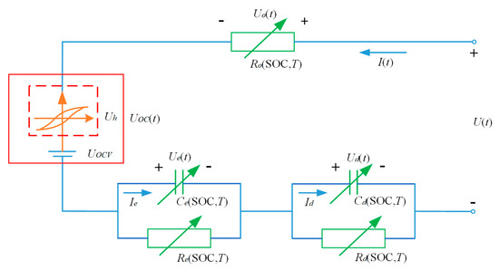
Figure 5.
Temperature–hysteresis equivalent circuit model.
According to the electric circuit model, the Kirchhoff equation is formulated as follows:
Model output equation:
U(t) = UOC(t) + Uo(t) + Ue(t) + Ud(t)
UOC(t) = UOCV(t) + Uh(t)
In order to simulate the characteristics of batteries more accurately, Equation (10) and (11) are discretized:
where, and .
The current integration method is used to estimate the battery SOC. The calculation of SOC is as shown:
Equation (12) is discretized as follows:
According to Equations (8)–(11) and (13), the discretized state space equations are established as follows:
where denotes the SOC of the battery at the moment k, η(T) denotes the coulomb efficiency, denotes the nominal capacity of the battery at temperature T, τ is the sampling period, is the system noise of the battery model, and is the measurement noise of the battery terminal voltage.
3. Battery SOC and SOP Joint Estimator
3.1. SOC Estimation Based on the AUKF Method
The noise covariance was a fixed value when using the unscented Kalman filter (UKF) for battery SOC estimation. However, the noise was continually changing during battery charging and discharging, which caused the estimation result to be unstable. In order to solve this problem, the AUKF algorithm was used to estimate the battery SOC [10]. The AUKF algorithm is shown in Table 1.

Table 1.
Algorithm of adaptive unscented Kalman filter 1.
3.2. SOP Estimation Under Multiple Constraints
3.2.1. Current Constraint
In the temperature–hysteresis model, we proposed the Thevenin equivalent circuit with hysteresis voltage put to use. The battery terminal voltage was composed of the following parts: Open-circuit voltage (considering hysteresis) , ohmic voltage , and polarization voltages and . It was stipulated that the current value was positive when the battery was charging and negative when discharging. The SOP estimation based on the current constraint was to use current as the single constraint. Starting from time , the power battery charged or discharged at a constant current within pulse time . According to the ECM, the equation of the terminal voltage and the polarization voltages and are as follows:
Then we need to predict the change of the battery terminal voltage during pulse charging and discharging. It is assumed that the parameters in the battery model are unchanged during the pulse time Δt. Meanwhile, is the maximum charging current and is the maximum discharging current, thus that the charge peak terminal voltage and discharge peak terminal voltage at time are as follows:
3.2.2. Voltage Constraint
When the battery was charged and discharged under voltage constraint, in order to make sure the battery would not be over-charged or over-discharged, it was necessary to make the terminal voltage of the battery reach the presetting cut-off voltage at the end of the predicted time. According to the model we proposed, the variation of the battery terminal voltage after a pulse charging and discharging time was as follows:
where , and are the polarization voltage value and current value before the start of the pulse process. Because the OCV does not change much during the pulse process, we assume that and are equal. According to Equation (28), is replaced by the maximum charge voltage and the cut-off discharge voltage , then the maximum charging current and the maximum discharging current can be obtained as follows:
where and are polarization voltages estimated from the battery model.
3.2.3. SOC Constraint
SOP estimation under SOC constraints was based on the maximum SOC or minimum SOC constraints during battery operation to obtain the charge and discharge peak current of power battery, and then calculated the peak power. In order to protect the safety and performance of batteries in practical applications, we needed to specify the SOC range of batteries. Therefore, assuming that the upper limit of SOC for battery charging was , the lower limit of SOC for discharging was , and the pulse charge and discharge time was . According to the current integration method, the following equation can be obtained:
Based on the temperature–hysteresis model built in this paper, and are the coulomb efficiency and nominal capacity at temperature T, respectively. The charge peak current and the discharge peak current under SOC constraint are as follows:
3.2.4. Multiple Constraints
SOP estimation results under single constraint may exceed the extreme value of SOP estimation under other constraints, which will lead to performance degradation and reduction of battery life. Therefore, this paper used multiple constraints to estimate the battery’s peak power. This method can significantly improve the accuracy of the estimation and ensure the safety of the battery thus that the battery can operate better.
In the case of the above single constraint, the maximum charge and discharge current can be obtained by calculation. Assume that and are used to represent the nominal maximum charge and discharge current of batteries, respectively, then the maximum charge and discharge current based on multiple constraints is as follows:
Combined with the battery terminal voltage , the peak power of the battery under multiple constraints can be obtained as follows:
3.3. Model-Based SOC and SOP Joint Estimator
Based on the model-based SOC and SOP estimators mentioned above, we propose a joint estimator for these two states. The proposed method consists of 3 parts, including the establishment of temperature–hysteresis model, SOC estimation based on the AUKF algorithm, and SOP estimation under multiple constraints. Variables are passed through different modules to form a complete framework, as shown in Figure 6.
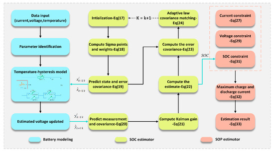
Figure 6.
The flowchart of the model-based SOC and state of power (SOP) estimator.
4. Verification and Discussion
4.1. Model Identification and Verification
The configuration of the test bench is drawn in Figure 7, which contains four components: (1) High-low temperature test box: It can control the battery operated under the designed temperatures. (2) 18,650 LiFePO4 lithium-ion batteries: It can verify the proposed algorithm. (3) ITS5300 battery charge and discharge test system: It can make the battery work under the designed loading profiles and measure real-time data. (4) Host computer: It can record the measurement data and carry out the simulation experiments by Matlab Simulink (R2016a, MathWorks, Natick, MA, USA).
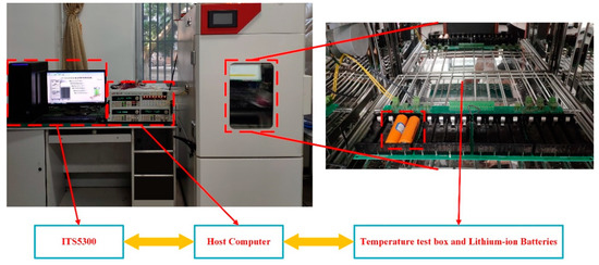
Figure 7.
Test bench.
This study will perform a characteristic test for a short period of the battery life cycle, thus we do not consider the battery aging phenomenon. Since the ITS5300 battery test system requires more than one cell to collect field data, two cells were connected in series as a battery pack during the experiment, and then three battery packs were used for the experimental data collection. The nominal capacity of each battery pack was 1.4 Ah, and the nominal voltage was 6.4 V. In order to protect the battery safety, 7 V and 4.2 V were used as the charging cutoff voltage and discharging cutoff voltage, respectively. Finally, we can get the experimental results of three battery packs, and then find the mean value for the model parameter identification, SOC estimation, and SOP estimation.
4.1.1. Model Parameters Identification
The temperature-based capacity model parameters can be solved by using the capacity data of the battery at different temperatures [32], as shown in Table 2. Temperature-based hysteresis model parameters can be obtained by using OCV data at different temperatures and SOC points [33], as shown in Table 3.
Table 2.
Parameters of the temperature-based capacity model.
Table 3.
Parameters of the temperature-based hysteresis voltage model.
The SOC–OCV data at different temperatures are averaged to obtain the final data for fitting as shown in Table 4. We fit data using the SOC–OCV model expressed by the Equation (34) [34]. The results are shown in Figure 8 and the parameter identification results are: A1 = −713.1, A2 = 3210, A3 = −6049, A4 = 6192, A5 = −3741, A6 = 1358, A7 = −289.7, A8 = 34.03, M = 4.736.
Table 4.
OCV at different SOC.
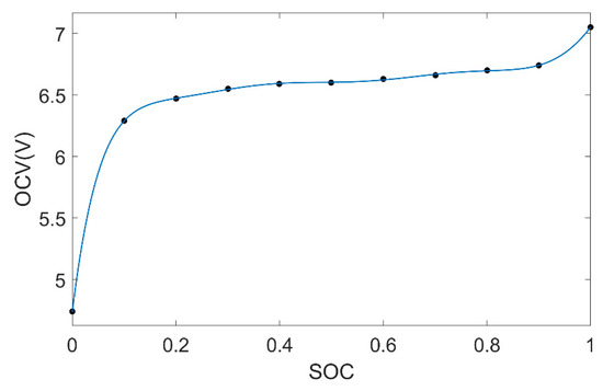
Figure 8.
SOC–OCV fitting curve.
The temperature–hysteresis model includes five unknown parameters: , , , , and . We can identify these parameters according to the system input and output data. This paper adopts the parameter direct identification algorithm, which is to use the Parameter Estimation function of the Matlab toolbox to identify the battery parameters automatically. When the error between the simulated output and the measured data reaches a predetermined threshold, the identified model parameters are saved.
The model parameters were identified by the pulse discharge current and voltage data. Firstly, set the initial parameters of the model and the range of parameters. Then the parameters were optimized by the method of nonlinear least squares. Finally, the discharge current was input into the model, and the parameters were estimated dynamically according to the fitting degree between the simulated output voltage and the actual voltage. The higher the fitting precision is, the more accurate the parameters are. In order to identify the parameters at different temperatures, the current value of the battery measured at different temperatures is used as model input. Figure 9 shows the identification results for the polarization capacitances. It can be seen that both polarization capacitances have a significant correlation with the temperature. At the same SOC, the polarization capacitances increased as the temperature rises.
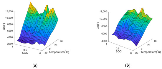
Figure 9.
Polarization capacitance identification results at different temperatures: (a) Electrochemical polarization capacitor; (b) concentration polarization capacitor.
The identification result of polarization resistances is shown in Figure 10. The polarization resistances decreased as the temperature increased. The ohmic resistance identification result is shown in Figure 11. It can be seen that the internal ohmic resistance decreased with the increase of temperature. At the same temperature, when the SOC was in the range from 10% to 90%, the ohmic resistance changed little; when the SOC was greater than 90% or less than 10%, the ohmic resistance increased rapidly.
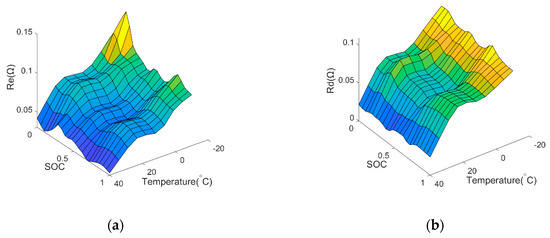
Figure 10.
Polarization resistance identification results at different temperatures: (a) Electrochemical polarization resistance; (b) concentration polarization resistance.
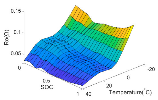
Figure 11.
Ohmic resistance identification results at different temperatures.
By analyzing the identification results of the battery model parameters, we can know that the battery parameters in this paper are variable at different temperatures and SOCs. Consequently, it is not easy to obtain the equation by the fitting curve. Therefore, the look-up table method is used to obtain the parameters in the process of state estimation.
4.1.2. Model Verification Under Constant Temperature Condition
According to the battery parameter identification results, the battery temperature–hysteresis model was built by Matlab Simscape. Then we used the improved DST profiles to verify the battery model under constant and variable temperature conditions separately. The DST test was a typical test cycle for power batteries, and it was often used to verify battery models and estimation algorithms [35]. In this paper, we improved the DST test according to the experimental conditions, and Figure 12 shows the current profiles of the improved DST cycles in this experiment. The batteries were placed in the 25 °C temperature test box, and the model output was compared with the test voltage to verify the accuracy of the model used in the present analysis. In addition, the second-order RC model without hysteresis was compared with the model proposed in this paper to verify the compensation effect of temperature–hysteresis model.
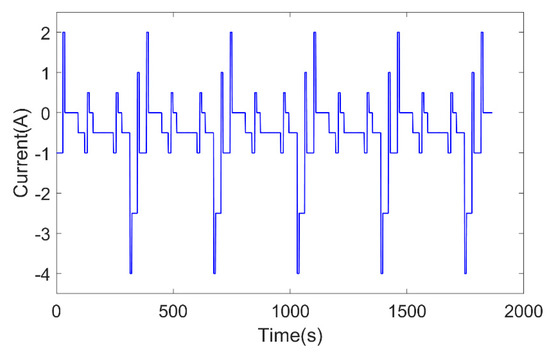
Figure 12.
Dynamic stress test (DST) profiles at 25 °C.
In this paper, the identification results at 25 °C were used as simulation model parameters. Figure 13 shows the simulation voltage curves of two different models under constant temperature conditions, where the blue curve is the terminal voltage actually measured in the experiment, the green curve is the output voltage of the temperature–hysteresis model, and the red curve is the output voltage of the second-order RC model without the hysteresis. Comparing the two simulation results, the simulation voltage of the proposed temperature–hysteresis model was closer to the measured value than that of the model without hysteresis. And the conventional second-order RC model without hysteresis cannot simulate the battery terminal voltage change in time during the charge and discharge conversion process. Figure 14 shows the output voltage error of two simulation models. It can be seen that the absolute error of the temperature–hysteresis model output voltage was less than 0.02V, while that of the second-order RC model output voltage was within 0.03V. The error of the latter model was obviously higher than that of the former model, which verified the validity of the temperature–hysteresis model at a constant temperature.
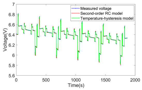
Figure 13.
Battery models output and measured voltage at 25 °C.
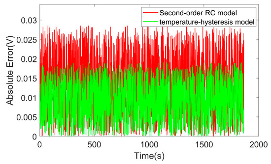
Figure 14.
Battery models output error at 25 °C.
4.1.3. Model Verification Under Variable Temperature Conditions
To verify the accuracy of the battery model under variable temperature conditions, firstly, we needed to place the batteries in the temperature test box with an initial temperature of 18 °C for 12h. During the experiment, the temperature of the temperature test box rose from 18 °C to 36 °C, and then remained at 36 °C until the end of the experiment. Finally, the battery model was verified by the improved DST profiles under variable temperature conditions shown in Figure 15, where the red curve represents the temperature change of the test box and the blue curve indicates the improved DST profiles.
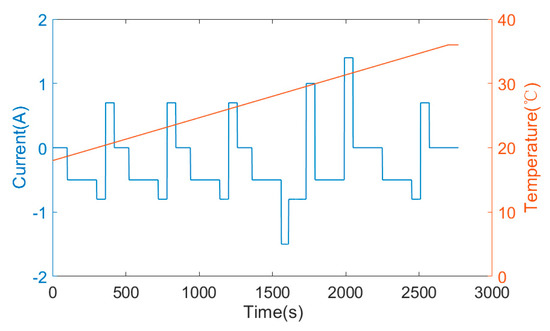
Figure 15.
Improved DST profiles under variable temperature conditions.
Under variable temperature conditions, the parameters of the model will be updated in real time following the change of the temperature and the SOC. Figure 16 shows the simulation voltage curves of the models under variable temperature conditions. The difference between the simulation output of the second-order RC model and the measured voltage was obvious, while the output of the temperature–hysteresis model could still accurately simulate the terminal voltage. Figure 17 shows the absolute error of the terminal voltage of two models under variable temperature conditions. The absolute error of the temperature–hysteresis model was stable below 0.026V. However, the absolute error of the second-order RC model increased obviously at variable temperatures. The maximum absolute error was 0.083V, and the error fluctuated greatly. Therefore, we can know that the compensation effect of the temperature–hysteresis model was more significant at various temperatures.
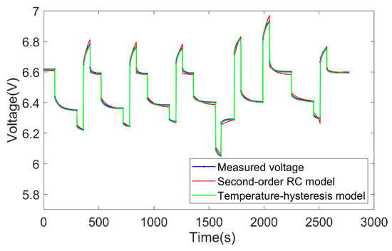
Figure 16.
Battery models output and measured voltage under variable temperature conditions.
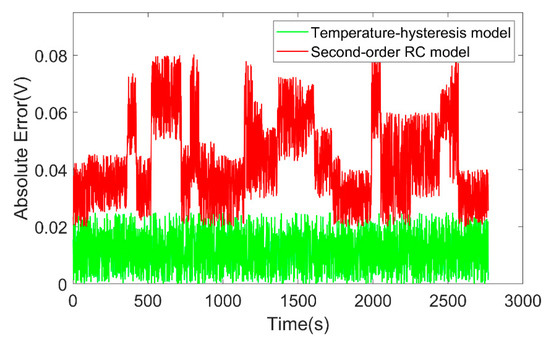
Figure 17.
Battery models output error curve under variable temperature conditions.
4.2. Verification of the SOC and SOP Joint Estimation
4.2.1. Verification of the SOC Estimation
The paper used the DST profiles in Figure 12 to estimate the SOC at a constant temperature. The SOC was estimated based on the AUKF algorithm using the temperature–hysteresis model and the second-order RC model, respectively. The initial parameters of the AUKF algorithm are shown in Table 5. As can be seen from Figure 18, the SOC estimation using the temperature–hysteresis model was closer to the value of the reference.
Table 5.
Parameters of the adaptive unscented Kalman filter (AUKF) algorithm.
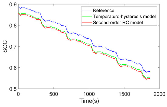
Figure 18.
SOC estimation based on different models under DST profiles at 25 °C.
Figure 19 shows the error of two SOC estimation algorithms. The estimation error of the conventional second-order RC model was significantly higher than that of the temperature–hysteresis model. The maximum estimated error of the SOC using the temperature–hysteresis model was 0.0288, and the root mean square error (RMSE) was 0.0262. The maximum estimated error of the second-order RC model was 0.0356, and the RMSE was 0.0321. Therefore, the AUKF algorithm based on the temperature–hysteresis model was more accurate for SOC estimation.
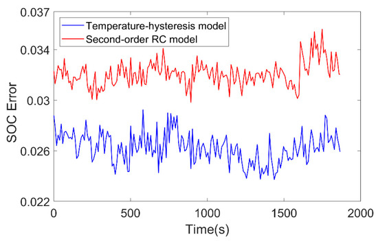
Figure 19.
SOC estimation error at 25 °C.
The current profiles in Figure 15 are used as the input of the model to verify the SOC estimation at variable temperatures. Likewise, the temperature still rose from 18 °C to 36 °C and then remained unchanged. The initial parameters of the AUKF algorithm are shown in Table 5. The first stage was in the stationary state thus that the SOC remained constant in the initial stage. Then the SOC changed from the second stage of the working condition. The SOC estimation results based on two models at variable temperature are shown in Figure 20, and the estimation error is shown in Figure 21. It can be seen that the SOC estimation based on the temperature–hysteresis model was better than that based on the second-order RC model. However, the error of both methods was increased compared with the error under constant temperature condition. It was caused by the more complex change of battery parameters under variable temperature conditions. The maximum error based on the temperature–hysteresis model was 0.0371, the RMSE was 0.0317. The maximum error based on the second-order RC model was 0.0489, the RMSE was 0.0436. The results showed that the AUKF algorithm based on the temperature–hysteresis model still had high precision under variable temperature, and the robustness of the temperature–hysteresis model was verified. This is mainly because the internal parameters of the proposed model can be updated with temperature thus that the estimation accuracy of the SOC is greatly improved compared with the second-RC model. Moreover, the SOC estimation value is used as the basis for the peak power estimation algorithm.
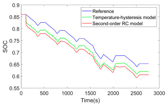
Figure 20.
SOC estimation based on different models under variable temperature conditions.
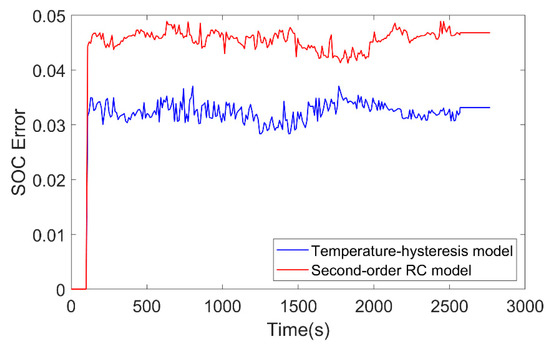
Figure 21.
SOC estimation error under variable temperature conditions.
4.2.2. Verification of the SOP Estimation
The current profiles of the DST cycles are used as an input to reflect the actual dynamic characteristics of the battery. The operating time of a single DST was 354 s. As shown in Figure 22, five DST cycles were used for the battery test. Figure 23 shows the terminal voltage profiles of the DST cycles. The model parameters involved in the calculation used the identification results in Section 4.1.1. The charge and discharge peak current under multiple constraints can be obtained by Equation (32).
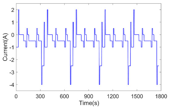
Figure 22.
Current profiles under DST test.
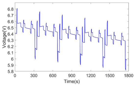
Figure 23.
Voltage profiles under DST test.
Two cells in series were used as experimental samples. It is necessary to ensure the safety of the battery during pulse charge and discharge. Therefore, according to the parameters given by the battery manufacturer, we assumed that the maximum battery charge current was 2.8 A and the maximum discharge current was 7 A under the current constraint; the charge cut-off voltage was 7 V, and the discharge cut-off voltage was 4.2 V under the voltage constraint; the upper limit of SOC was 0.9, and the lower limit was 0.1 under the SOC constraint. The simulation pulse time was 10 s. According to the actual operating state of the battery, the initial SOC value was set to 0.86, and the battery capacity was 1.397 Ah.
To calculate the peak power, we should analyze the peak currents under various constraints. Figure 24 shows the multi-constrained charge peak current curves. The current profiles under each constraint condition can be seen clearly. Current changes under SOC constraints are more obvious than those under voltage constraints and current constraints. Since the initial SOC value was 0.88, the voltage constraint condition will be reached quickly during charging. The current under the SOC constraint is useful only at the beginning of charging. As the battery charging continues, the voltage constraint begins to play a dominant role. However, the actual current will be limited by the current constraint, when the actual current exceeds the peak current specified by the manufacturer. Therefore, to ensure the safety of the battery and to slow down the aging of the battery, the minimum current under three constraints is taken as the peak current, as shown by the purple curve in Figure 24.
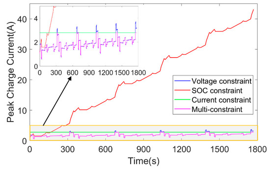
Figure 24.
Multi-constrained battery charge peak current curve.
Figure 25 shows the multi-constrained discharge peak current curves obtained by simulation. In the simulation time, the multi-constraint discharge peak current mainly depends on the current value under the voltage constraint and the current constraint. In this paper, the whole discharge process cannot be shown because only five DST cycles were used. However, with the analysis of Figure 24, the current based on the SOC constraint at the later stage of the discharge will be smaller than the current under other constraints. The peak current at this time mainly depends on the SOC constraint.
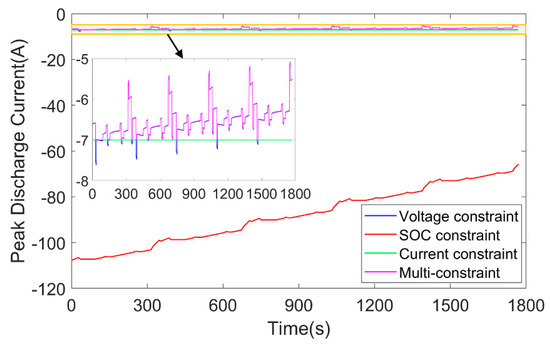
Figure 25.
Multi-constrained battery discharge peak current curve.
Figure 26 shows the prediction results of charging peak power, and Figure 27 shows the prediction results of discharging peak power. As can be seen from Figure 27, the peak power value of the battery decreased significantly from 315 s to 345 s due to the large discharge current, and the discharge ability of the battery became weak in a short time. When the small discharge current was used, the peak power value increased, and the discharge ability of the battery became strong. Compared with the conventional HPPC method, the peak charge and discharge power value obtained by the multi-constraint method was much smaller, and this was because the model adopted by the HPPC method was much simpler, and the current constraint and the SOC constraint were not taken into account in the practical calculation. Therefore, the proposed peak power prediction method based on multi-constraint conditions was more effective.
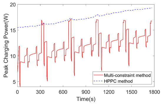
Figure 26.
Charge peak power prediction curve.
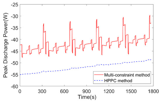
Figure 27.
Discharge peak power prediction curve.
5. Conclusions
In a short summary, we have presented physical perspectives of the energy output characteristics of lithium iron phosphate battery from both mathematical modeling and experimental tests. The effect of temperature and hysteresis on battery modeling is analyzed, then the temperature–hysteresis model based on the second-order RC model is established. And the direct identification method is used to identify battery parameters. The modeling simulation is completed in MATLAB. Experimental results show that the error of the temperature–hysteresis model is smaller than that of the traditional RC model under constant and variable temperature conditions. The state space equation of the SOC estimation is established by introducing a temperature–hysteresis model, and the battery SOC is estimated online based on the AUKF algorithm. The peak current of the battery is calculated based on the current-voltage-SOC joint constraints, and then the peak power is estimated. The simulation results show that the reliability of peak power estimation using the multi-constraint method is higher than that using the HPPC method. This method effectively solves the problem of inaccurate battery SOP estimation caused by the single constraint condition during the charge and discharge process. To the best of our knowledge, this may be the first trial on an in-depth theoretical analysis of the dynamic charging state of lithium-ion batteries under different temperatures exploiting multi-state joint estimator, thus that any relevant conclusion that comes out in the present study can provide useful guidelines on the elaborate design of temperature–hysteresis model-based battery device in the broad context of energy conversion systems for modern industrial field. It is our belief that these results are to spur interdisciplinary research in power system, energy harvesting, and battery vehicles, and cause positive interactions among applied mathematicians, electrical engineers, and physical scientists in the near future.
Author Contributions
X.L. and X.Z. contributed to the developing the algorithm, conducting the experiments, and writing of this article. G.W. and W.L. reviewed and revised the paper.
Funding
This project is financially supported by the Key Research and Development Program of Shaanxi Province (NO. 2019ZDLGY15-04-02, No. 2018ZDCXL-GY-05-07-02, No. 2019GY-083, and No. 2019GY-059) and the Fundamental Research Funds for the Central Universities (No. 300102329502).
Conflicts of Interest
The authors declare no conflict of interest.
Nomenclature
| Symbols | |
| Q | battery capacity: mAh |
| T | battery temperature, °C |
| η | coulombic efficiency |
| I | load current, A |
| maximum hysteresis voltage, V | |
| hysteresis voltage, V | |
| Sgn(·) | sign function |
| open-circuit voltage, V | |
| ohmic resistance, Ω | |
| electrochemical polarization resistance, Ω | |
| concentration polarization resistance, Ω | |
| electrochemical polarization capacitance, F | |
| concentration polarization capacitance, F | |
| τ | sampling period, s |
| system state vector | |
| system input vector | |
| system noise | |
| measurement noise | |
| Subscripts and Superscripts | |
| k | time step index |
| chg | charge |
| dis | discharge |
| max | maximum |
| min | minimum |
| ^ | estimation value |
| Abbreviations | |
| SOC | state of charge |
| SOP | state of power |
| EV | electric vehicle |
| AUKF | adaptive unscented Kalman filter |
| UKF | unscented Kalman filter |
| ECM | equivalent circuit model |
| OCV | open-circuit voltage |
| HPPC | hybrid pulse power characteristic |
| DST | dynamic stress test |
| RMSE | root mean square error |
| C | discharge rate |
References
- Un-Noor, F.; Padmanaban, S.; Mihet-Popa, L.; Mollah, M.N.; Hossain, E.; Sciubba, E. A Comprehensive Study of Key Electric Vehicle (EV) Components, Technologies, Challenges, Impacts, and Future Direction of Development. Energies 2017, 10, 1217. [Google Scholar] [CrossRef]
- Lu, L.; Han, X.; Li, J.; Hua, J.; Ouyang, M. A review on the key issues for lithium-ion battery management in electric vehicles. J. Power Source 2013, 226, 272–288. [Google Scholar] [CrossRef]
- Hannan, M.A.; Lipu, M.S.H.; Hussain, A.; Mohamed, A. A review of lithium-ion battery state of charge estimation and management system in electric vehicle applications: Challenges and recommendations. Renew. Sustain. Energy Rev. 2017, 78, 834–854. [Google Scholar] [CrossRef]
- Plett, G.L. Extended Kalman filtering for battery management systems of LiPB-based HEV battery packs: Part 3. State and parameter estimation. J. Power Sources 2004, 134, 277–292. [Google Scholar] [CrossRef]
- Xiong, R.; Cao, J.; Yu, Q.; He, H.; Sun, F. Critical Review on the Battery State of Charge Estimation Methods for Electric Vehicles. IEEE Access 2018, 6, 1832–1843. [Google Scholar] [CrossRef]
- Sun, F.; Xiong, R.; He, H. Estimation of state-of-charge and state-of-power capability of lithium-ion battery considering varying health conditions. J. Power Sources 2014, 259, 166–176. [Google Scholar] [CrossRef]
- Wang, Y.; Zhang, C.; Chen, Z. A method for joint estimation of state-of-charge and available energy of LiFePO4 batteries. Appl. Energy 2014, 135, 81–87. [Google Scholar] [CrossRef]
- Plett, G.L. High-performance battery-pack power estimation using a dynamic cell model. IEEE Trans. Veh. Technol. 2004, 53, 1586–1593. [Google Scholar] [CrossRef]
- Lei, P.; Zhu, C.; Wang, T.; Lu, R.; Chan, C. Online peak power prediction based on a parameter and state estimator for lithium-ion batteries in electric vehicles. Energy 2014, 66, 766–778. [Google Scholar]
- Zhang, W.; Shi, W.; Ma, Z. Adaptive unscented kalman filter based state of energy and power capability estimation approach for lithium-ion battery. J. Power Sources 2015, 289, 50–62. [Google Scholar] [CrossRef]
- Nejad, S.; Gladwin, D.T.; Stone, D.A. A systematic review of lumped-parameter equivalent circuit models for real-time estimation of lithium-ion battery states. J. Power Sources 2016, 316, 183–196. [Google Scholar] [CrossRef]
- He, H.; Zhang, X.; Xiong, R.; Xu, Y.; Guo, H. Online model-based estimation of state-of-charge and open-circuit voltage of lithium-ion batteries in electric vehicles. Energy 2012, 66, 310–318. [Google Scholar] [CrossRef]
- Smith, K.A.; Rahn, C.D.; Wang, C.Y. Model-Based electrochemical estimation and constraint management for pulse operation of Lithium Ion batteries. IEEE Trans. Control Syst. Technol. 2010, 18, 654–663. [Google Scholar] [CrossRef]
- Chen, S.; Fu, Y.; Mi, C.C. State of Charge Estimation of Lithium Ion Batteries in Electric Drive Vehicles Using Extended Kalman Filtering. IEEE Trans. Veh. Technol. 2013, 62, 1020–1030. [Google Scholar] [CrossRef]
- Guo, M.; Kim, G.H.; White, R.E. A three-dimensional multi-physics model for a Li-ion battery. J. Power Sources 2013, 240, 80–94. [Google Scholar] [CrossRef]
- Zhang, X.; Wang, Y.; Wu, J.; Chen, Z. A novel method for lithium-ion battery state of energy and state of power estimation based on multi-time-scale filter. Appl. Energy 2018, 216, 442–451. [Google Scholar] [CrossRef]
- Tian, Y.; Xia, B.Z.; Wang, M.W.; Sun, W.; Xu, Z.H. Comparison study on two model-based adaptive algorithms for SOC estimation of lithium-ion batteries in electric vehicles. Energies 2014, 7, 8446–8464. [Google Scholar] [CrossRef]
- Zhu, L.; Sun, Z.; Dai, H.; Wei, X. A novel modeling methodology of open circuit voltage hysteresis for LiFePO4 batteries based on an adaptive discrete Preisach model. Appl. Energy 2015, 155, 91–109. [Google Scholar] [CrossRef]
- Hu, X.S.; Li, S.B.; Peng, H. A comparative study of equivalent circuit models for Li-ion batteries. J. Power Sources 2012, 198, 359–367. [Google Scholar] [CrossRef]
- Yoon, S.; Hwang, I.; Lee, C. Power capability analysis in lithium ion batteries using electrochemical impedance spectroscopy. J. Electroanal. Chem. 2011, 655, 32–38. [Google Scholar] [CrossRef]
- Feng, T.; Yang, L.; Zhao, X.; Zhang, H.; Qiang, J. Online identification of lithium-ion battery parameters based on an improved equivalent-circuit model and its implementation on battery state-of-power prediction. J. Power Sources 2015, 281, 192–203. [Google Scholar] [CrossRef]
- Idaho National Engineering & Environmental Laboratory. Battery Test Manual for Plug-in Hybrid Electric Vehicles; Assistant Secretary for Energy Efficiency and Renewable Energy (EE) Idaho Operations Office: Idaho Falls, ID, USA, 2010. [Google Scholar]
- Pesaran, A.A. Battery thermal models for hybrid vehicle simulations. J. Power Sources 2002, 110, 377–382. [Google Scholar] [CrossRef]
- Sun, F.; Xiong, R.; He, H.; Li, W.; Aussems, J.E.E. Model-based dynamic multi-parameter method for peak power estimation of lithium-ion batteries. Appl. Energy 2012, 96, 378–386. [Google Scholar] [CrossRef]
- Fleischer, C.; Waag, W.; Bai, Z.; Sauer, D.U. Self-learning state-of-available-power prediction for lithium-ion batteries in electrical vehicles. In Proceedings of the 2012 IEEE Vehicle Power and Propulsion Conference (VPPC), Seoul, Korea, 9–12 October 2012; pp. 370–375. [Google Scholar]
- Xiong, R.; Sun, F.; Gong, X.; He, H. Adaptive state of charge estimator for lithium-ion cells series battery pack in electric vehicles. J. Power Sources 2013, 242, 699–713. [Google Scholar] [CrossRef]
- Plett, G.L. Extended Kalman filtering for battery management systems of LiPB-based HEV battery packs: Part 2. Modeling and identification. J. Power Sources 2004, 134, 262–276. [Google Scholar] [CrossRef]
- Zheng, F.; Xing, Y.; Jiang, J.; Sun, B.; Kim, J.; Pecht, M. Influence of different open circuit voltage tests on state of charge online estimation for lithium-ion batteries. Appl. Energy 2016, 183, 513–525. [Google Scholar] [CrossRef]
- Zhang, C.; Li, K.; Deng, J.; Song, S. Improved Real-time State-of-Charge Estimation of LiFePO4 Battery Based on a Novel Thermoelectric Model. IEEE Trans. Ind. Electron. 2016, 64, 654–663. [Google Scholar] [CrossRef]
- Thele, M.; Bohlen, O.; Sauer, D.U.; Karden, E. Development of a voltage-behavior model for NiMH batteries using an impedance-based modeling concept. J. Power Sources 2018, 175, 635–643. [Google Scholar] [CrossRef]
- Xia, B.; Wang, H.; Tian, Y.; Wang, M.; Sun, W.; Xu, Z. State of Charge Estimation of Lithium-Ion Batteries Using an Adaptive Cubature Kalman Filter. Energies 2015, 8, 5916–5936. [Google Scholar] [CrossRef]
- Xiong, R.; Sun, F.; Gong, X.; Gao, C. A data-driven based adaptive state of charge estimator of lithium-ion polymer battery used in electric vehicles. Appl. Energy 2014, 113, 1421–1433. [Google Scholar] [CrossRef]
- Barai, A.; Widanage, W.D.; Marco, J.; McGordon, A.; Jennings, P. A study of the open circuit voltage characterization technique and hysteresis assessment of lithium-ion cells. J. Power Sources 2015, 295, 99–107. [Google Scholar] [CrossRef]
- Yu, Q.; Xiong, R.; Lin, C.; Shen, W.; Deng, J. Lithium-ion Battery Parameters and State-of-Charge Joint Estimation Based on H infinity and Unscented Kalman Filters. IEEE Trans. Veh. Technol. 2017, 66, 8693–8701. [Google Scholar] [CrossRef]
- Zhang, C.; Jiang, J.; Zhang, W.; Sharkh, S.M. Estimation of State of Charge of Lithium-Ion Batteries Usedin HEV Using Robust Extended Kalman Filtering. Energies 2012, 5, 1098–1115. [Google Scholar] [CrossRef]


© 2019 by the authors. Licensee MDPI, Basel, Switzerland. This article is an open access article distributed under the terms and conditions of the Creative Commons Attribution (CC BY) license (http://creativecommons.org/licenses/by/4.0/).