Hardware-in-the-Loop Validation of Model Predictive Control of a Discrete Fluid Power Power Take-Off System for Wave Energy Converters

Abstract

Model predictive control based wave power extraction algorithms have been developed and found promising for wave energy converters. Although mostly proven by simulation studies, model predictive control based algorithms have shown to outperform classical wave power extraction algorithms such as linear damping and reactive control. Prediction models and objective functions have, however, often been simplified a lot by for example, excluding power take-off system losses. Furthermore, discrete fluid power forces systems has never been validated experimentally in published research. In this paper a model predictive control based wave power extraction algorithm is designed for a discrete fluid power power take-off system. The loss models included in the objective function are based on physical models of the losses associated with discrete force shifts and throttling. The developed wave power extraction algorithm directly includes the quantized force output and the losses models of the discrete fluid power system. The experimental validation of the wave power extraction algorithm developed in the paper shown an increase of 14.6% in yearly harvested energy when compared to a reactive control algorithm.

1. Introduction

Energy produced by ocean waves has yet not become a commercial viable technology mainly due to the high cost of energy. Therefore, research projects considering wave energy converters are diversified into numerous topics regarding for example, structural mooring, system controls, power electronics, hydrology and fluid power technology—all with the aim of reducing the cost of energy as reviewed in, for example, Reference [1].

In the current work focus is on the heart of the Wave Energy Converter (WEC) namely the Power Take-Off (PTO) system, which converts the energy of ocean waves into easily distributable electrical energy. Specificity, the current study focuses on Wave Power Extraction Algorithms (WPEAs) that controls the PTO system. The PTO is controlled by the WPEA to harvest as much energy as possible from the ocean waves and, in connection to energy harvesting, it is relevant to distinguish between absorbed and harvested energy. The absorbed energy is the mechanical energy fed into the WEC from the ocean wave and the harvested energy is the energy output from the WEC to the power grid, that is, the difference between absorbed and harvested energy is the losses in the conversion.

For point absorber WECs characterized by the float being small compared to the dominant wave length a reactive WPEA has been the preferred as reported in References [2,3]. Model Predictive Control (MPC) algorithms have recently been proposed and investigated with increasing attention from the wave energy research community, see for example, References [4,5,6,7,8,9,10] and consult Reference [11] for a comprehensive overview of MPC in general WEC’s. Linear MPC has been developed and simulated in, for example, References [4,5,9] for an ideal PTO system applied to a point absorber WEC. In most work on MPC control, the PTO system efficiency has been omitted, while the absorbed mechanical energy has been in focus rather than the useful harvested output energy. In Reference [10], a PTO system was modelled using a linear damping term as a loss model but the actual PTO system leading to this simplified loss model is not discussed.

Though not shown for MPC the losses in the PTO system is of high importance when designing WPEAs and evaluating energy performance. In References [12,13,14] physical based models of the PTO system have been included at shown significant influence on chosing the optimal WPEA coefficients and production evaluation.

An inherent concern with MPC algorithms is the demands to calculation/computational effort. The MPC algorithm solves an optimization problem in each time step which requires many evaluations of a (complicated) system model. For systems with slow dynamics (high time constants) this is not a large problem but for systems with small time constants and high eigen-frequencies the MPC sampling time must be low, leaving short time for the evaluation of control algorithms.

As outlined research focusing on MPC for wave energy has increased significantly in the recent years. Little work, however, has been reported on experimental validation of MPC algorithms. Especially, validations of algorithms including PTO system losses in the objective function are almost absent in the research on MPC for WEC. In Reference [15] an experimental validation is reported using a simple loss model to represent the power calculation. Details of the physical PTO system with this loss model is not discussed. Nevertheless, Reference [15] presents an experimental validation including both the MPC algorithm and a on-line running prediction model for the wave excitation force. In Reference [16] the same authors discuss a MPC based WPEA for a WEC featuring an imperfect PTO system such energy losses in the power conversion is considered.

MPC strategies have been proposed in, for example, References [17,18] for digital fluid power systems but also in this research area the lack of experimental validation and tests are distinct. This lacking validation of MPC algorithms including physical based loss models exists both in the field of wave energy and digital fluid power system.

In this paper focus in on experimental validation of MPC applied to a discrete fluid power PTO system. The discrete PTO system is based on the discrete displacement cylinder technology that features a multi-chamber cylinder connected to a number of constant pressure lines, see for example, Reference [19]. The feasibility of MPC based WPEA’s for discrete PTO systems was established in Reference [20], where promising performance was reported. The current paper focuses on how prediction models may be simplified to allow models that are computationally light. The current paper reports MPC based WPEA’s feasible for real-time implementation in the proposed setup where the MPC sample time is 350 ms and a proper wave prediction is available. Prediction of wave excitation forces are beyond the scope of this paper but interested reader may consult Reference [21,22] for insight in this important topic.

The paper is organized as follows: first, an overview of the experimental setup is given together with a brief review of the discrete PTO system. Next, the MPC configuration is discussed with focus on prediction model simplification and energy loss modelling. Then, an introduction to the real-time implementation and accompanying issues is given. Finally, the conclusion sums up the findings regarding the experimental validation of MPC based WPEA’s for discrete fluid power PTO systems for wave energy converters.

Discrete Power Take-Off System

The PTO system studied in this paper was originally proposed for a multiple-point absorber wave energy converter, see Reference [3]. Each absorber is attached to an arm hinged at a fixed structure and in overall terms energy is harvested by the relative motion between the absorber arm and the fixed structure. Figure 1 illustrates the system. Each set of float arm, multi-chamber cylinder and valve manifold constitutes a unit named a primary stage. As indicated in Figure 1, multiple primary stages are connected to a common secondary stage consisting of three pressure lines each equipped with a number of accumulators, a fixed displacement fluid power motor, an electrical generator and a frequency converter for grid connection.

A key advantage of such a topology is that inevitable (but phase shifted) variations in the power production of the individual absorbers do not propagate directly into the secondary stage which in turn leads to a more smooth operation of the fluid power motor and the generator.

It may be noted that the two ports of the fluid power motor are connected to the low ($p_{\mathrm{L},1}$) and high pressure ($p_{\mathrm{L},3}$) lines, respectively. The intermediate pressure ($p_{\mathrm{L},2}$) floats and, as detailed in Reference [3], proper secondary control is needed to stabilize this pressure line.

2. Experimental Setup

A test bench capable of testing “full scale” PTO systems for wave energy converters was designed at The Department of Energy Technology at Aalborg University, see Figure 2.

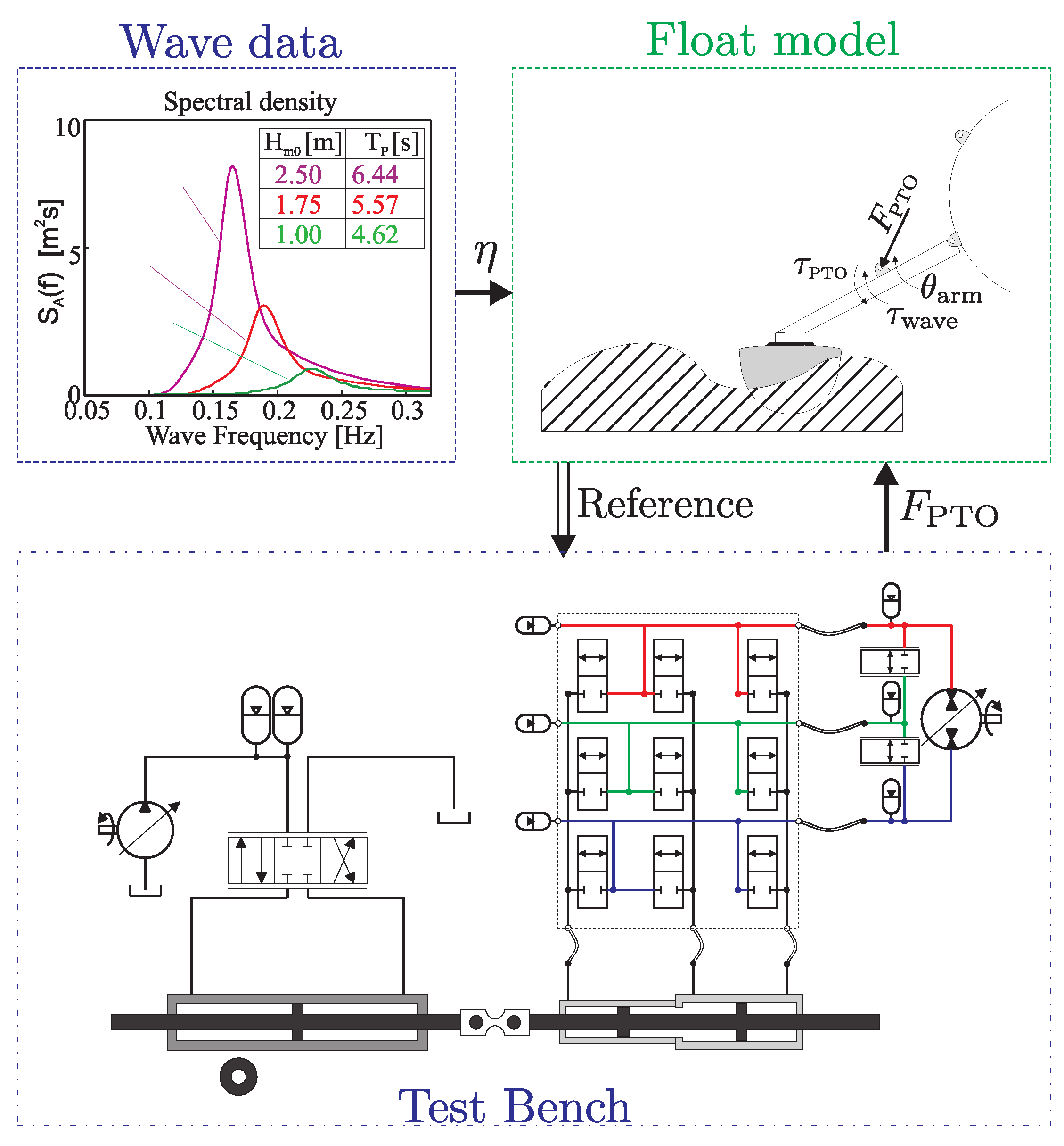
The test bench is designed to emulate the movement of a point absorber wave energy converter as the one in Figure 1 under various wave conditions. Various PTO systems may be installed in the test bench to harvest energy of the movement. The load system emulating wave forces and float dynamics is controlled with trajectory tracking. The trajectory is however generated with an on-line simulation model, of the WEC float, taking wave climate data and on-line PTO force measurements as inputs. The function of the test bench is illustrated in Figure 3. A predefined wave time series is together with real-time measurements of the applied PTO force fed to the float model that then in real-time outputs a float movement applied as reference trajectory for the test bench load system.

2.1. Test Bench

The test bench mechanical design is elaborated in Reference [23]; Reference [24] may be consulted for a thorough description of the control system.

The load system emulating the float movement consists of a 250/180/3000 mm symmetric cylinder controlled with a 4/3 servo valve supplied by a 375 kW hydraulic power unit. The supply line is equipped with two 28 L accumulators installed to handle peak wave conditions. The load system is capable of emulating the movement of a 5 m diameter point absorber float operating in 3 m significant wave height. A model of the test bench was developed, analysed and validated in Reference [25].

2.2. Discrete Displacement Cylinder

The PTO system tested is a Discrete Displacement Cylinder (DDC) system including a three chamber cylinder, three pressure lines and a valve manifold as investigated in Reference [20]. The valve manifold connecting the cylinder and the pressure lines is fitted with on/off valves matched in size with the corresponding cylinder area, such the pressure drop is 5 bar across each fully open on/off valve at a steady piston velocity of 0.5 m/s. The PTO system topology is developed for multi-point absorbed WECs, see Reference [3], that is, the secondary part of the PTO system (pressure lines, hydrostatic motor and electrical generator) is designed to handle flow from multiple primary stages. The secondary stage of the test bench PTO system is however designed to control the line pressure and not designed for energy harvesting. The PTO part installed in the test bench is designed and used for testing of the primary stages of DDC systems. The system data for the primary stage tested are given in

Table 1. Discrete Displacement Cylinder (DDC) PTO system parameters. (The sign of the area indicates the force direction of each chamber.)

$A_1=(+)235$ cm${}^2$	$p_{L.1}=20$ bar	$k_{v.1}=705\frac{L/\min }{\sqrt{5\mathrm{bar}}}$
$A_2=(-)122$ cm${}^2$	$p_{\mathrm{L}.2}=100$ bar	$k_{\mathrm{v}.2}=366\frac{\mathrm{L}/\min }{\sqrt{5\mathrm{bar}}}$
$A_3=(-)87$ cm${}^2$	$p_{\mathrm{L}.3}=180$ bar	$k_{\mathrm{v}.3}=261\frac{\mathrm{L}/\min }{\sqrt{5\mathrm{bar}}}$

.

2.3. Wave Data

The wave data utilised in the test bench is based on the scatter diagram given in

Table 2. Scatter diagram for utilized wave climates and naming of the sea states. The sea states used are mark with bold face.

Total 1.0		${\mathit{T}}_{0.2}$ (s)
		3.5	4.5	5.5
$H_{\mathrm{m}0}$ (m)	0.75	0.233(11)	0.146(14)	-
	1.25	0.083(12)	0.206(15)	-
	1.75	-	0.133(16)	0.071(18)
	2.25	-	0.038(17)	0.049(19)
	2.75	-	-	0.041(20)

. The scatter diagram shows the probability of a wave climate given by the significant wave height, H${}_{\mathrm{m}}$, and the peak wave period, T${}_{\mathrm{wp}}$. Furthermore the naming of the sea state used in the experimental validation of MPC based WPEA’s are shown in the bold face (i.e., sea state 17 and 20 are not employed). Sea states 17 and 20 are not used due to the low probability and high requested piston velocities which are unfeasible for the current test bench.

The wave time series for the experimental test are generated by filtering white noise as described in Reference [3]. The filtering is performed such the power density of the wave series follow the often used Pierson-Moskowitz spectrum. As this filtering process will generate a new wave series each time it is run a fair comparison is ensured by generating one time series per sea state. Three examples of the spectrum are seen in Figure 4.

An estimate of yearly energy production may be calculated by the weighted sum of the energy output in the seven sea states by the probability shown in the scatter diagram, a estimation of production and down time must though be included. However in this study the individual production numbers for each sea state is compared.

2.4. Float Model

The float model utilised for online generation of the tracking reference for the load cylinder is briefly introduced based on the work of References [2,20]. The notation used follows Figure 1. A block diagram is see in Figure 5 and the transfer function representation is

$$\frac{{\theta }_{arm}\left(s\right)}{{\tau }_{\mathrm{pto}}\left(s\right)+{\tau }_{\mathrm{ext}}\left(s\right)}=\frac{1}{(J_{\mathrm{arm}}+J_{\mathrm{add},\infty })s^2+K_{\mathrm{r}}\left(s\right)s+k_{\mathrm{res}}},$$

(1)

with the coefficients in

Table 3. Float model parameters.

$J_{\mathrm{arm}}$	2.45 $·{10}^6$	$\left({\mathrm{kgm}}^2\right)$
$J_{\mathrm{add},\infty }$	1.32 $·{10}^6$	$\left({\mathrm{kgm}}^2\right)$
3pt] $K_{\mathrm{res}}$	14 $·{10}^6$	$(\mathrm{Nm}/\mathrm{rad})$
$[b_5,\cdots ,b_0]$	$[0.01,1.44,62.4,816,1310,144]·{10}^4$
$[a_5,\cdots ,a_0]$	$[0.0010,0.0906,1.67,6.31,13.3,9.18]$

. The model inputs are the torque from the PTO system and the ocean wave ${\tau }_{\mathrm{pto}}$ and ${\tau }_{\mathrm{ext}}$ respectively. Note, the radiation damping $K_{\mathrm{r}}\left(s\right)$ is model with a 5’th order linear approximation and the Archimedes-gravity term uses the linearisation constant $k_{\mathrm{res}}$.

A Bode diagram of the float model (1) is shown in Figure 6. Note the second order like nature and the resonance peak at 0.285 Hz indicating the float arm eigen frequency.

3. Model Predictive Control of a Discrete PTO System

In the context of a PTO system, the overall control problem is to maximize the energy output in varying sea states by clever manipulation of the PTO force, which in our case must be selected from a pool of 27 values. The pool of 27 forces originates from the combination of 3 cylinder areas and 3 pressure levels ($3^3=27$). Traditionally, a controller is tuned off-line based on ideas such as reactive control [2] and mapping techniques are used to accommodate quantization of the controller output [3].

As an alternative to such an indirect approach, to attack both the energy maximization problem and the force level quantization problem, the variant of closed-loop control model known as either receding horizon control or model predictive control has two appealing characteristics for use in a WEC with a discrete PTO system—as detailed in Reference [26], MPC allows direct handling of constraints such as actuator and state limitations—and also, due to the use of an on-line optimization strategy, MPC should be able to address the energy maximization problem directly during run time. One should however note that model predictive control is clearly based on a system model, why the model quality highly influences the results. Proper models of the wave-float interaction, PTO system dynamics and losses and wave prediction are such essential for MPC based WPEAs.

The overall idea of MPC is to compute the future controller outputs (i.e., the system inputs) by solving an optimizing problem on each time step of duration $T_{\mathrm{S}}$. More specifically, the strategy for a discrete-time MPC involves three steps:

• Measure (or partially estimate) the full system state $x\left(k\right)$ at the current sampling time $t\left(k\right)$.
• Find the N optimal future system inputs

  $$\begin{array}{c}\hfill {\mathcal{U}}_k=[u\left(k\right),u(k+1),\cdots u(k+N-1)]\end{array}$$

  (2)

  by solving an optimization problem over a finite time horizon $T_{\mathrm{H}}=T_{\mathrm{s}}N$ by using a prediction model to estimate the future system states

  $$\begin{array}{c}\hfill {\mathcal{X}}_k=[x(k+1),x(k+2),\cdots x(k+N)]\end{array}$$

  (3)

  based on the initial state $x\left(k\right)$, the future inputs ${\mathcal{U}}_k$ besides a prior estimates of future disturbances
• Apply only the first optimal controller output $u\left(k\right)$ to the system and loop back to step 1 for the next sampling instant.

Figure 7 illustrates the used notation and the MPC principle: at time $t\left(k\right)$ the actual state $x\left(k\right)$ is available and an optimal future controller output vector ${\mathcal{U}}_k$ is determined as outline in Step 2 above. Using ${\mathcal{U}}_k,$ the predicted future state becomes ${\mathcal{X}}_k$ as shown in the bottom part of Figure 7. The first element $u\left(k\right)$ is immediately applied to the system and as indicated the actual state trajectory may deviate from the prediction leading to another initial state in the next sampling interval starting at $t(k+1)=t\left(k\right)+T_{\mathrm{s}}$.

In the following subsections, the configuration of the MPC based WPEA is described in detail.

3.1. Prediction Models

The prediction model derived in Reference [20] is based on the continuous state space model (4) for the float arm movement when given input $\tilde{u}=u+w\triangleq {\tau }_{\mathrm{pto}}+{\tau }_{\mathrm{ext}}$. Note, that this is the total input inform of both the excitation and PTO torque.

$$\begin{array}{c}\begin{array}{cc}\hfill \left[\begin{array}{c}{\ddot{\theta }}_{arm}\\ {\dot{\theta }}_{arm}\\ {\dot{\tau }}_{\mathrm{rad},\mathrm{kr}}\\ {\dot{x}}_{kr,1}\\ {\dot{x}}_{kr,2}\\ {\dot{x}}_{kr,3}\\ {\dot{x}}_{kr,4}\end{array}\right]& =\left[\begin{array}{ccccccc}0& \frac{-k_{res}}{J_{tot}+J_{tot}}& \frac{-1}{J_{tot}+J_{tot}}& 0& 0& 0& 0\\ 1& 0& 0& 0& 0& 0& 0\\ b_1-a_1{b}_0& 1& -a_1& 1& 0& 0& 0\\ b_2-a_2{b}_0& 1& -a_2& 0& 1& 0& 0\\ b_3-a_3{b}_0& 1& -a_3& 0& 0& 1& 0\\ b_4-a_4{b}_0& 1& -a_4& 0& 0& 0& 1\\ b_5-a_5{b}_0& 1& -a_5& 0& 0& 0& 0\end{array}\right]\left[\begin{array}{c}{\dot{\theta }}_{arm}\\ {\theta }_{arm}\\ {\tau }_{\mathrm{rad},\mathrm{kr}}\\ x_{kr,1}\\ x_{kr,2}\\ x_{kr,3}\\ x_{kr,4}\end{array}\right]+\left[\begin{array}{c}\frac{-1}{J_{tot}+J_{tot}}\\ 0\\ 0\\ 0\\ 0\\ 0\\ 0\end{array}\right]\tilde{u}\hfill \\ \hfill {\dot{\theta }}_{\mathrm{arm}}& =\left[\begin{array}{cccc}1& 0& \cdots & 0\end{array}\right]{\left[\begin{array}{ccccccc}{\dot{\theta }}_{arm}& {\theta }_{arm}& {\tau }_{\mathrm{rad},\mathrm{kr}}& x_{kr,1}& x_{kr,2}& x_{kr,3}& x_{kr,4}\end{array}\right]}^T\hfill \end{array}\end{array}$$

(4)

The prediction of future states is based on a discrete state space model of the float dynamics (4). The states at the next time instant $x(k+1)$, where k is the current sample is given as:

$$\begin{array}{cc}\hfill x(k+1)& =Ax\left(k\right)+B\tilde{u}\left(k\right)\hfill \\ \hfill & =Ax\left(k\right)+B\left(u\left(k\right)+w\left(k\right)\right)\hfill \\ \hfill y\left(k\right)& =Cx\left(k\right),\hfill \end{array}$$

(5)

where $u\left(k\right)$ relates to controllable input (${\tau }_{\mathrm{pto}}$) and $w\left(k\right)$ is the uncontrollable disturbance (${\tau }_{\mathrm{ext}}$) and $\tilde{u}\left(k\right)$ combines the two inputs. Also, A, B and C are the discrete representation of the system matrices of (4) using a zero order hold discretization with the sample time $T_{\mathrm{S}}$, equal to the controller sample time.

The prediction model predicting future states in the prediction horizon was derived to the matrix equation:

$$\begin{array}{cc}\hfill \underset{{\mathcal{X}}_k}{\underbrace{\left[\begin{array}{c}x(k+1)\\ x(k+2)\\ ⋮\\ x(k+N)\end{array}\right]}}=\underset{\mathrm{P}}{\underbrace{\left[\begin{array}{c}A\\ A^2\\ ⋮\\ A^N\end{array}\right]}}x\left(k\right)& +\underset{\mathrm{H}}{\underbrace{\left[\begin{array}{cccc}B& 0& \cdots & 0\\ AB& B& \cdots & 0\\ ⋮& ⋮& \ddots & ⋮\\ A^{N-1}B& A^{N-2}B& \cdots & B\end{array}\right]}}\underset{{\mathcal{U}}_k}{\underbrace{\left[\begin{array}{c}u\left(k\right)\\ u(k+1)\\ ⋮\\ u(k+N-1)\end{array}\right]}}\hfill \\ \hfill & +\underset{\mathrm{H}}{\underbrace{\left[\begin{array}{cccc}B& 0& \cdots & 0\\ AB& B& \cdots & 0\\ ⋮& ⋮& \ddots & ⋮\\ A^{N-1}B& A^{N-2}B& \cdots & B\end{array}\right]}}\underset{{\mathcal{W}}_k}{\underbrace{\left[\begin{array}{c}w\left(k\right)\\ w(k+1)\\ ⋮\\ w(k+N-1)\end{array}\right]}}\hfill \end{array}$$

(6)

The future system outputs ${\mathcal{Y}}_k$ may be stated as:

$$\underset{{\mathcal{Y}}_k}{\underbrace{\left[\begin{array}{c}y(k+1)\\ y(k+2)\\ ⋮\\ y(k+N)\end{array}\right]}}=\underset{{\mathrm{C}}_{\omega }}{\underbrace{\left[\begin{array}{cccc}C& 0& \cdots & 0\\ 0& C& \cdots & 0\\ ⋮& ⋮& \ddots & ⋮\\ 0& 0& \cdots & C\end{array}\right]}}{\mathcal{X}}_k$$

(7)

Note that to model the future state, ${\mathcal{X}}_k$, in the prediction horison, $T_{\mathrm{N}}=T_{\mathrm{s}}N$, of N samples the initial state $x\left(k\right)$ and the future system inputs ${\mathcal{U}}_k$ and disturbances ${\mathcal{W}}_k$ are requested.

Simplified Prediction Model

The prediction model (5) has seven system states, that is, the model (6) predicting the future states over the prediction horizon has $7N$ elements. Each objective function evaluation during optimization of the control input requires the simulation model to be evaluated. Hence, the execution time of the prediction model must be low leading to construction of a simplified system model. The model simplification is performed by assuming that the radiation damping function, $K_{\mathrm{r}}\left(s\right)$, is constant that is, the float model is reduced to a second order system:

$$\begin{array}{c}\hfill \left[\begin{array}{c}{\dot{\theta }}_{\mathrm{arm}}\\ {\ddot{\theta }}_{\mathrm{arm}}\end{array}\right]=\left[\begin{array}{cc}0& 1\\ \frac{-{\mathrm{k}}_{\mathrm{res}}}{{\mathrm{J}}_{\mathrm{tot}}+{\mathrm{J}}_{\infty }}& \frac{-{\mathrm{B}}_{\mathrm{rad}}}{{\mathrm{J}}_{\mathrm{tot}}+{\mathrm{J}}_{\infty }}\end{array}\right]\left[\begin{array}{c}{\theta }_{\mathrm{arm}}\\ {\dot{\theta }}_{\mathrm{arm}}\end{array}\right]+\left[\begin{array}{c}0\\ \frac{1}{{\mathrm{J}}_{\mathrm{tot}}+{\mathrm{J}}_{\infty }}\end{array}\right]\tilde{u}\end{array}$$

(8)

Recall that $\tilde{u}=u+w\triangleq {\tau }_{\mathrm{pto}}+{\tau }_{\mathrm{ext}}$. Then, the simplified prediction model is such constructed from (8), similar to how (6) is constructed using (4).

The validity of the simplified model and the choice of $B_{\mathrm{rad}}$ is investigated by a comparative simulation study, where a MPC based WPEA is employed using the 7th order and $2^{\mathrm{nd}}$ prediction model, respectively. The constant radiation damping in the $2^{\mathrm{nd}}$ order model is varied to investigate the influence of choosing an “optimal” value. The simulation comparison is conducted with the three wave climates shown in Figure 4, inducing small, medium and large waves. The average harvested power using the simple $2^{\mathrm{nd}}$ order model is seen in Figure 8 normalized with the average power harvested with the 7th order model.

As seen in Figure 8 from a harvested energy point of view, the MPC model based the second order prediction model may perform similar to the MPC utilizing the seven order prediction model, if the radiation damping coefficient is selected carefully. It is furthermore seen that the same radiation damping coefficient may be used to get a rather good approximation in all three wave climates. To see the effect in terms of computational time, a test is conducted calculating the future system states as shown i (6) for the 7th order and $2^{\mathrm{nd}}$ order model. For the test a prediction length of $N=10$ is chosen. Each case is calculated 1000 times and the average is compared. The average calculation time was 90 $\mathsf{\mu }$s and 20 $\mathsf{\mu }$s for the 7th and $2^{\mathrm{nd}}$ order model, respectively. The average calculation time is thus reduced by a factor of almost four without major impact on the harvested energy estimate.

3.2. MPC Objective Functions

The MPC based WPEA is designed to calculate the optimal control inputs to the PTO system. But how is optimal defined. In this study the harvested energy is maximized by aiming at a large amount of absorbed energy and a low energy loss. The objective function to maximize in the MPC is formulated as the absorbed energy minus the energy losses in the PTO system. The energy loss model may be constructed with various complexity and detail level. Four loss models of increasing complexity are developed leading to five objective functions (9)–(13) given as:

$$\begin{array}{cc}\hfill & J_1\left({\mathcal{T}}_{k,\mathrm{pto}}\right)=E_{\mathrm{abs}}\hfill \end{array}$$

(9)

$$\begin{array}{cc}\hfill & J_2\left({\mathcal{T}}_{k,\mathrm{pto}}\right)=E_{\mathrm{abs}}-E_{\mathrm{loss}.\mathrm{s}}(1,0)\hfill \end{array}$$

(10)

$$\begin{array}{cc}\hfill & J_3\left({\mathcal{T}}_{k,\mathrm{pto}}\right)=E_{\mathrm{abs}}-E_{\mathrm{loss}.\mathrm{s}}(x_{\mathrm{c}},0)\hfill \end{array}$$

(11)

$$\begin{array}{cc}\hfill & J_4\left({\mathcal{T}}_{k,\mathrm{pto}}\right)=E_{\mathrm{abs}}-E_{\mathrm{loss}.\mathrm{s}}(x_{\mathrm{c}},{\dot{x}}_{\mathrm{c}})\hfill \end{array}$$

(12)

$$\begin{array}{cc}\hfill & J_5\left({\mathcal{T}}_{k,\mathrm{pto}}\right)=E_{\mathrm{abs}}-E_{\mathrm{loss}.\mathrm{s}}(x_{\mathrm{c}},{\dot{x}}_{\mathrm{c}})-E_{\mathrm{loss}.\mathrm{t}}\left({\dot{x}}_{\mathrm{c}}\right)\hfill \end{array}$$

(13)

The energy losses included in the models are shifting and throttling losses as described in Reference [20] ($E_{\mathrm{loss}.\mathrm{s}}$ is losses associated with shifting the PTO force and $E_{\mathrm{loss}.\mathrm{t}}$ is losses associated with throttling). As this paper focuses on experimental implementation of the MPC based WPEA’s the calculation time of the objective function is important because computational time is a limited recurse in a real-time implementation. One may note that $J_2$ includes shifting losses assuming no chamber volume change (${\dot{x}}_{\mathrm{c}}=0$) and that the piston is in its center position ($x_{\mathrm{c}}=1$) while $J_3$ includes variations in piston position. $J_2$ allows the loss to be included by a lookup table and also the cylinder states do not need to be calculated which leads to lower computational time compared with the remaining objective functions. In $J_4$ the loss model is depending both on the piston position and velocity while $J_5$ further includes throttling losses likewise depending on ${\dot{x}}_{cyl}$.

The future force levels (the controller outputs) are thus optimized subject to the objective functions:

$$\begin{array}{c}\hfill {max{J}_i}_{{\mathcal{T}}_{k,\mathrm{pto}}}\end{array}$$

(14)

where the future PTO torque values requested by the controller are ${\mathcal{T}}_{k,\mathrm{pto}}=[{\tau }_{\mathrm{pto}}\left(k\right),{\tau }_{\mathrm{pto}}(k+1),\dots ,{\tau }_{\mathrm{pto}}(k+N-1)]$. The optimal PTO torque for sample instant i is ${\tau }_{\mathrm{pto}}\left(i\right)$. Note that the optimization problem is an unconstrained bounded integer problem, such no constraints functions are enforced. The design space is however bounded to 27 integer values given by the three pressure levels and the three piston areas.

3.3. Loss Models

The loss models used below in the current study were introduced in Reference [20] and developed and investigated in Reference [27,28]. The losses associated with force shifts are:

$$\begin{array}{cc}{E}_{\mathrm{loss}.\mathrm{s}}(x_{\mathrm{c}},{\dot{x}}_{\mathrm{c}})=\hfill & {\displaystyle \sum _{i=1}^3}{\displaystyle \sum _{n=1}^N}\left[\frac{1}{2}\frac{{\left(p_{i,n}-p_{i,n-1}\right)}^2}{\beta }{V}_{\mathrm{c},i,n}\right.\hfill \\ & +\frac{1}{2}\left(p_{i,n}-p_{i,n-1}\right){\dot{V}}_{\mathrm{c},i,n}{\mathrm{T}}_{\mathrm{p}}\hfill \\ & \left.+\frac{13}{70}\frac{{\left(p_{i,n}-p_{i,n-1}\right)}^2}{\beta }{\dot{V}}_{\mathrm{c},i,n}{\mathrm{T}}_{\mathrm{p}}\right],\hfill \end{array}$$

(15)

where $p_{i,n}$ is the pressure in and ${\dot{V}}_{\mathrm{c},i,n}$ is the volume of the i’th chamber at time instant n. ${\mathrm{T}}_{\mathrm{p}}$ is the time duration of a force shift. The chamber pressures for each time step is found from a lookup table mapping the force level to corresponding chamber pressures.

In addition, the energy loss associated with static throttling over a prediction horizon ${\mathrm{T}}_{\mathrm{H}}$ is

$$E_{\mathrm{loss},\mathrm{t}}\approx T_s\left(|{\mathcal{Y}}_k{|}^T{k}_{\mathrm{v}.\mathrm{t}}\left({\mathcal{Y}}_k\circ {\mathcal{Y}}_k\right)\right),$$

(16)

where ∘ denotes component-wise multiplication. The total throttling loss coefficient is given as:

$$k_{\mathrm{v}.\mathrm{t}}=\sum _{i=1}^3\frac{A_i^3}{k_{\mathrm{v}.i}^2}$$

(17)

Note that the power losses from throttling are depending on the pressure drop across the valve

$$\sum _{i=1}^3\frac{A_i^2}{k_{\mathrm{v}.i}^2}\left({\mathcal{Y}}_k\circ {\mathcal{Y}}_k\right)$$

(18)

and the flow through the valve

$${\mathcal{Y}}_k{A}_i.$$

(19)

The energy loss is found via first order Euler integration with $T_{\mathrm{s}}$.

4. Real-Time Implementation of Model Predictive Control

The MPC based WPEAs are implemented in the existing test bench control system programmed in LabVIEW and executed on a LabVIEW Real-Time Target. The optimization algorithm is hand-written in c-code and compiled to a dynamic link library (DLL) using LabWindows/CVI and linked to the LabVIEW application.

The procedure for solving the MPC based WPEA is listed below:

• Sample system variables, $x\left(k\right)$, and estimate wave excitation torque, ${\tau }_{\mathrm{ext}}\left(k\right)$
• Calculate the optimal future system inputs, ${\mathcal{U}}_k$
• Apply the system input, $u\left(k\right)$
• Wait until the next sampling instance and repeat

It should be noted that a computational delay is inevitably introduced depending on the time it takes to solve the optimization problem. To guarantee that a solution is available at all samples the optimization algorithm is stopped if it has not converged within the sample time. In this case, the next instance of the previous solution is applied $u(k+1)$ for the u calculated in the prior run. An essential part of MPC is the optimization algorithm which is described in the following.

Optimization Algorithm

The optimization algorithm used in this MPC formulation is a differential evolution (DE) algorithm similar to the one used in Reference [20] and initially presented in Reference [29]. Differential evolution is chosen primarily as it is capable of dealing with discrete optimization problems (see for example, Reference [30]) such as Equations (9)–(13). It may be noted that in-house implemented variants of the DE algorithm have proven very efficient for solving mixed continuous-integer engineering design problems as reported in, for example, Reference [31]. As this current study focuses mainly on proving feasibility no effort have been put into implementing and benchmarking specialized optimization algorithms because our general-purpose DE algorithm has proven useful and relatively simple to implement on a real-time application as well.

The general idea of differential evolution is to initialize a population of $NP$ designs and evolve the population through mutations and ranking using objective function values until the population converges towards a common solution. This evolution of generations is continued until the population fulfils a convergence criterion. To decrease the computation time some modifications to the original algorithm are conducted: a warm start procedure is utilized to initialize the population in the neighbourhood of the previous optimal solution as it is assumed that the next optimal solution falls in the vicinity of the previous optimal solution. This is supported by the fact that MPC algorithm only applies the first design variable before time is advance by one sample where the optimization problem is solved again. In other words that the next optimal solution covers the time from $t(k+1)$ to $t(k+1+\mathrm{N}),$ where the current solution relates to time interval $t\left(k\right)$ to $t(k+\mathrm{N})$. A downside of imposing the warm start procedure is that the search area of the solution space is significantly decreased which may result in not finding the global optimum if this is not in the neighbourhood of the previous solution.

The DE algorithm used has five parameters to be set: The population size (concurrent, different designs in a generation) is $NP$ while the numbers of generations utilized in the convergence criterion is K. The evolution of one generation to the next is controlled by the cross over coefficient, F, and $CR$ deciding the amount of poor solutions to discard. The final parameter is the convergence tolerance, $ϵ$.

The parameters $NP$, F, $CR$, K and $ϵ$ are all tuned in an effort of obtaining efficient performance for all objective functions. The parameters are chosen identical for all objective functions and are shown in

Table 4. Parameters used in the differential evolution algorithm.

NP	F	CR	K	$\mathit{ϵ}$
400	0.7	0.9	5	${10}^{-8}$

.

It should be noted that the optimization algorithm does not guarantee finding a global optimum.

5. Results

The experimental investigations of the MPC based WPEA’s are performed on the described PTO test bench. The online float model running on the testbench setup is the 7’th order model given in (1) and Figure 5, whereas the prediction model used in the MPC based WPEA’s is the simplified $2\mathrm{nd}$ order model in (8). Figure 9 shows measurements of the PTO cylinder position, PTO cylinder chamber pressures and the applied PTO force, while applying MPC2 in sea state 15.

The MPC based WPEA is tested in the seven sea states indicated in Table 2 for all the objective functions described in Equations (9)–(13). A benchmark WPEA based on reactive control is likewise run in the seven sea states for establishing a baseline for comparison [2]:

$$F_{\mathrm{pto}}=B_{\mathrm{pto}}{\dot{x}}_{\mathrm{cyl}}+K_{\mathrm{pto}}{x}_{\mathrm{cyl}},$$

(20)

where the coefficients $B_{\mathrm{pto}}$ and $K_{\mathrm{pto}}$ are depending on the sea state. In this way, the benchmark controller is optimized to maximise the harvested power in the actual sea state.

Below, the MPC based WPEA’s are denoted MPCi, index i being the subscript of the corresponding objective function.

Average absorbed and harvested power are used as evaluation figures and furthermore the PTO efficiency is included. The average power is calculated over the time period T covering 100 wave periods. Using the measured PTO force and piston velocity, the average absorbed power is calculated from

$$P_{\mathrm{abs}}=\frac{1}{T}{\int }_0^T{\dot{x}}_{\mathrm{cyl}}{F}_{\mathrm{pto}}dt$$

(21)

Unfortunately, no measurements of the flow in the low pressure line is available so the harvested power has to be approximated. This is done using an average of two ways to estimate $P_{\mathrm{har},1}$ and $P_{\mathrm{har},2}$. The first estimate $P_{\mathrm{har},1}$ calculates the harvested power relative to the low pressure line by

$$P_{\mathrm{har},1}=\frac{1}{T}{\int }_0^T{Q}_{\mathrm{H}}\left(p_{\mathrm{H}}-p_{\mathrm{L}}\right)+Q_{\mathrm{M}}\left(p_{\mathrm{M}}-p_{\mathrm{L}}\right)dt,$$

(22)

where $Q_{\mathrm{H}}$ and $Q_{\mathrm{M}}$ are the flow into the high, medium and low pressure line respectively. Also, $p_{\mathrm{H}},p_{\mathrm{M}}$ and $p_{\mathrm{L}}$ are the pressure in the high, medium and low pressure lines, respectively.

The second estimate $P_{\mathrm{har},2}$ is based on approximation of the flow to the low pressure line as the cylinder velocity multiplied by the piston areas of the chambers connected to the low pressure line leading to

$$P_{\mathrm{har},2}=\frac{1}{T}{\int }_0^T{Q}_{\mathrm{H}}{p}_{\mathrm{H}}+Q_{\mathrm{M}}{p}_{\mathrm{M}}+{\tilde{Q}}_{\mathrm{L}}{p}_{\mathrm{L}}dt,$$

(23)

where ${\tilde{Q}}_{\mathrm{L}}={\tilde{Q}}_{\mathrm{L}}({\dot{x}}_{\mathrm{cyl}},A_i,u)$ is the approximated flow to the low pressure line.

The PTO efficiency is defined as:

$$\eta =\frac{P_{\mathrm{har}}}{P_{\mathrm{abs}}}$$

(24)

5.1. Comparison of Loss Models

To analyse the effect of including different detail levels of the loss model terms, the harvested power for the MPC based WPEAs are compared in Figure 10 for sea state 11, 15 and 18. The algorithms in the comparison are evaluated with a MPC sample time equal to 0.35 s and a 2.8 s time horizon ($T_{\mathrm{S}}=0.35$ s and $N=8$). The sample time and time horizon are chosen as a compromise between performance and computational time in the real-time system. Harvested power, absorbed power and conversion efficiency are tabulated for all MPC based WPEAs and the seven sea states in

Table 5. Harvested power, absorbed power and efficiency for five MPC based WPEAs for seven sea states.

		Sea State
		11	12	14	15	16	18	19
P${}_{\mathrm{har}}$ (kW)	MPC1	−2.3	1.8	1.1	8.4	16.0	19.0	26.4
	MPC2	1.3	5.2	3.3	10.1	17.7	20.6	27.7
	MPC3	1.1	5.1	2.9	10.1	17.7	20.7	27.9
	MPC4	1.4	5.5	3.0	10.2	18.2	20.7	28.1
	MPC5	1.5	5.6	3.1	10.3	18.4	20.9	28.8
P${}_{\mathrm{abs}}$ (kW)	MPC1	3.0	8.5	6.3	14.9	23.4	25.9	33.7
	MPC2	2.8	8.6	5.4	14.1	22.9	25.4	33.2
	MPC3	2.6	8.4	4.9	13.9	22.8	25.4	33.4
	MPC4	2.8	8.5	4.9	13.8	23.1	25.2	33.4
	MPC5	2.7	8.4	4.8	13.7	23.0	25.1	33.7
Eff (%)	MPC1	−78	22	18	56	68	73	78
	MPC2	45	61	61	72	77	81	83
	MPC3	42	61	59	72	78	82	84
	MPC4	51	64	62	74	79	82	84
	MPC5	54	67	65	75	80	83	85

.

As seen MPC1 harvests (solid bar) less power compared to the remaining MPCs for all sea states, indicating that loss models should be included to increase performance. One may note that MPC1 in fact has negative amount of harvested power for sea state 11, that is, the loss exceeds the absorbed power.

As only small difference between MPC2-MPC5 is observed, it is difficult to conclude if the more complex loss formulations increase the harvested power significantly. This may indicate that the loss models does not accurately describe the actual loss in the system or that the actual losses described by the more complex loss models are small in the current system design. The used valves are for example, large compared to the piston velocity yielding small throttling losses. Likewise the large dead volumes in the test bench PTO cylinder reduces the influence of difference in piston positions, yielding losses in MPC2 and MPC3 being close to equal.

To exemplify the effect of including a loss model in the MPC formulation, the PTO force reference is shown in Figure 11 using sea state 11.

As seen the MPC formulation without loss inclusion imposes more force steps compared to an MPC formulation that includes losses. In total MPC1 conducts 851 force steps for sea state 11 in comparison to 360 for MPC2 during the investigated time interval. The total number of force steps for MPC3, MPC4 and MPC5 are similar to MPC2. The difference in number of force steps appears as MPC1 will change force whenever a force yielding a higher power absorption is available. In contrary, MPC2-MPC5 all weigh the added absorbed power against the added losses associated with the requested force shift leading a much lower number of shifts of the force.

5.2. Computational Time

The computational time of each MPC iteration depends both of the maximum number of generations allowed and on the time is takes to evaluate the objective function, which in turn depends on the complexity of the loss model. As a consequence the computational time of the MPC based WPEAs are increasing when more loss terms are included. The computational time for each objective function is shown for sea state 14 in

Table 6. Computational time to ensure convergence for differential evolution (DE)-based MPC algorithm in sea state 14 with $T_s=0.35$ s and $T_H=2.8$ s.

	MPC
	1	2	3	4	5
Computational time per generation, (ms)	0.49	0.49	0.76	0.79	0.85
Total computational time, $T_{\mathrm{comp}}$ (ms)	16	45	71	79	85

.

The sea states not shown in Table 6 show similar trends except that the general computational time and number of generations decreases with increasing wave height. This may indicate that the optimisation problem is easier to solve for high-energy waves than for low-energy waves, which may be due to the limit on the available maximum force. The computational time for one generation indicates the computational burden of each objective function evaluation. As expected the computational burden increases with the complexity of the loss estimation. As seen the average computational time is well below the sample time of the MPC indicating that the number of design variables of the optimisation problem may be increased. The increased number of design variables may permit lowering the sample time or increasing the time horizon. In order to see how MPC may perform with higher number of design variables, MPC2 is utilised. In

Table 7. Harvested power and mean computational time for MPC2 for different T_s and $N_{\mathrm{late}}.$

		N
	${\mathit{T}}_{\mathit{s}}$ (ms)	8	10	12
$P_{\mathrm{har}}\left(\mathrm{kW}\right)$	250	7.95	9.16	10.30
	300	9.36	10.58	10.73
	350	10.16	10.61	10.15
$T_{\mathrm{comp}}\left(\mathrm{ms}\right)$	250	58	106	137
	300	47	77	109
	350	39	60	87
$N_{\mathrm{late}}(\%)$	250	0.8	5.2	18.3
	300	0.0	0.3	4.1
	350	0.0	0.1	0.5

the harvested power for different number of design variables and different sample times are shown for sea state 15. Here, $N_{\mathrm{late}}$ is the percentage of the number of occurrences where the optimisation algorithm did not converge within required time.

As seen it is possible to increase the harvested power by increasing the number of design variables instead of including more complex loss models. The number of design variables and the complexity of the loss model should be a compromise between performance and the limitations imposed by the computational time of the optimization algorithm combined with the computational power available for real-time implementation.

5.3. WPEA Performance

The performance for the MPC based WPEA are shown in Figure 12 compared to the benchmark WPEA based on reactive control. The results are given for the seven sea states in Table 2. The MPC algorithm employed is MPC${}_2$ with $N=10$ and $T_{\mathrm{S}}$ = 0.35 s, that is, the prediction horizon is 3.5 s. The MPC${}_2$ algorithm is chosen since the simpler energy loss model allows for better combination of MPC time step and prediction horizon than the more complex loss models.

The MPC based WPEA is in general seen to perform better compared to the reactive WPEA. For the lower sea states the WPEA’s perform similar while the MPC based WPEA performs significantly better in higher sea states. Even though the reactive control algorithm uses suboptimal control constants the MPCs ability to adjust to the variable amplitude and frequency is seen important for a high energy harvesting.

Weighing the average harvested power by the probability of the sea states, shown in Table 2 yields an average power production for the given site. Calculations show that MPC2 is able to increase the average yearly harvested power by 14.6% compared to the reactive WPEA in the test wave scatter.

6. Discussion

As MPC algorithms are computational demanding the prediction model has in the current experimental implementation been simplified to a great extent. Besides the simplified $2^{\mathrm{nd}}$ order float model the PTO system has been assumed ideal such that the commanded PTO force is available immediately. However, in reality the force dependents on the pressure level in the common pressure lines, which somewhat incorrectly was assumed constant. Furthermore, the pressure loss due to throttling are not accounted for in the force prediction. In addition to the imperfect force level, the PTO force dynamics are far from negligible as well, that is, a linear second order system with an eigenfrequency of 50 Hz would more accurately mimic the actual PTO force. This will, however, increase the complexity of the simulation model to be evaluated many times in real-time leading to an increase of the total MPC algorithm.

Likewise, the prediction loss model have been simplified to reduce the computational load. Whether or not the low benefit in including the more complex loss terms originates from the assumption of constant pressure lines, the ideal force dynamics or the overall fact that the models are too simple is at the moment unclear. The throttling loss is, however, due to the chosen valves insignificant, such the authors expect the throttling loss model to be essential for other DDC system designs.

Ideally, the full system model for the DDC system should be included in the prediction model but this will unfortunately significantly increase the computational requirements. Efforts on improving the precision of models and the calculation speed will surely enhance the MPC based algorithms.

As the current study focuses on proof of concept some initial efforts have been given to code optimization but it is certainly possible to reduce the MPC computational time further by a better implementation of the prediction and loss model and especially the core optimization algorithm itself. In addition, an optimization algorithm specially tailored for discrete MPC problems may reduce the calculation time as well.

7. Conclusions

This study validates that a MPC based WPEA can indeed be implemented in real-time and improve the energy output of a discrete displacement cylinder power take-off system. Based on the presented results it has been shown feasible to employ MPC based WPEA’s in a wave energy converter PTO system using DDC technology. The experimental validation has been performed on a test bench designed to test fluid-power PTO systems where the loading on the PTO system from the float was emulated based on an on-line simulation model.

The study showed that including a simple force shifting loss model improved the energy harvesting, especially in low energy waves where the losses are a large percentage of the absorbed energy. For the current system design the more complex loss models did not improve the energy harvesting significantly. This is may be explained by low throttling losses due to oversized valves and little position dependency of the shifting losses due to the large dead volume in the PTO cylinder. Poor precision of the loss models may be and other reason. A future simulation study may seek to investigate the significance of the various losses for varying system designs.

In the current study the prediction of the incoming wave torque was assumed ideal. Future studies on MPC based WPEA’s should quantify the requirements to precision for such wave prediction algorithms. This is an important topic because the wave prediction quality and accuracy directly couples in the MPC algorithm.

Even with the simplified system prediction and loss models the MPC based WPEA outperforms the suboptimal reactive WPEA. It was shown possible to maintain a MPC sample time of 0.35 s with a prediction horizon of 3.5 s on the setup used. The MPC2 algorithm showed to increase the average harvested power by 14.6% compared to the reactive WPEA, which illustrates the energy harvesting potentials of MPC methods.