Research and Application of Hybrid Wind-Energy Forecasting Models Based on Cuckoo Search Optimization

Abstract

Wind energy is crucial renewable and sustainable resource, which plays a major role in the energy mix in many countries around the world. Accurately forecasting the wind energy is not only important but also challenging in order to schedule the wind power generation and to ensure the security of wind-power integration. In this paper, four kinds of hybrid models based on cyclic exponential adjustment, adaptive coefficient methods and the cuckoo search algorithm are proposed to forecast the wind speed on large-scale wind farms in China. To verify the developed hybrid models’ effectiveness, wind-speed data from four sites of Xinjiang Uygur Autonomous Region located in northwest China are collected and analyzed. Multiple criteria are used to quantitatively evaluate the forecasting results. Simulation results indicate that (1) the proposed four hybrid models achieve desirable forecasting accuracy and outperform traditional back-propagating neural network, autoregressive integrated moving average as well as single adaptive coefficient methods, and (2) the parameters of hybrid models optimized by artificial intelligence contribute to higher forecasting accuracy compared with predetermined parameters.

1. Introduction

Fossil fuel resources are not renewable and are very limited, therefore, it is necessary to seek sustainable and clean energy resources. However, in practice, one problem with utilizing wind energy is that, compared with other electricity-generating methods, wind energy is not as steady and it is intermittent. Furthermore, if the electricity from wind energy accounts for a fairly large proportion of total electricity supply, the safe operation of the power grid may be threatened. Many factors, such air density around the wind farms and wind turbine characteristics, have an impact on the wind energy production. The use of energy storage systems can eliminate short-term disconnections from the grid of wind-energy sources [1]. Specifically, the amount of energy in wind is related with the cubic of the wind speed [2]. Therefore, the accuracy of wind-speed forecasting must be improved to attain more precise estimates of wind-power generation and thus better guide power dispatching and scheduling. This will to some extent promote the wind-energy industry to generate wind power more efficiently and ensure sustainable development.

Wind-speed forecasting methods can be divided by researchers into different fields contributing to develop models to forecast wind speed. For example, physical, statistical, or artificial intelligence models. Other models that involve multiple methods are also proposed, such as the combined models and hybrid models. The physical model utilizes wind farm and geographic information around the wind turbine to obtain the wind-speed data and other values of interest. It is usually very complex and has high precision and wide application in long-term prediction. The statistical model describes the mapping relationship between various parameters input by the system and the wind farm output, mainly including the time series method [3,4,5], exponential smoothing method [6], Kalman filtering method [7], regression method [8,9], empirical mode method [10,11,12,13] and so on.

Generally speaking, artificial intelligence models are the most widely used wind-speed forecasting models. For example, Blanchard and Samanta [14] proposed the non-linear autoregressive neural network method and non-linear autoregressive neural network with exogenous inputs method, which are two variations of artificial neural networks. Chitsazan et al. [15] utilizes the non-linear relationship between the internal states of echo state networks (ESN) and the proposed two methods for wind direction and speed forecasting. Compared with the classical ESN methods, the proposed method is computationally more efficient. It reduces the order of the weight matrices and has a smaller number of internal states.

A novel wind-speed forecasting method which utilizes an optimal model selection strategy is proposed by Zhou et al. [16]. The method first uses the improved boxplot to de-noise the data, then back propagation (BP), wavelet neural network (WNN), general regression neural network (GRNN) and adaptive network-based fuzzy inference system (ANFIS) are applied for the forecasting step, then finally, WIC is adopted to find the best model. Hu et al. [17] developed a hybrid model to do wind forecasting based on ensemble empirical mode decomposition (EEMD) and support vector machine (SVM), and the obtained experimental results reported an observable improvement of forecasting accuracy. Based on multi-scale dominant ingredient chaotic analysis, Fu et al. [18] present a novel hybrid method. It improved the hybrid GWO-SCA (IHGWOSCA) algorithm and extreme learning machine (ELM) for multi-step short-term wind-speed prediction. A new hybrid method which predicts the conditional quantile of wind speed was proposed by Zhang et al. [19]. This approach combines quantile regression and minimal gated memory network methods. They also discussed the feature selection and combination’s goal in constructing the optimal feature inputs. Li et al. [20] proposed a new wavelet packet decomposition (WPD)–Boost Elman neural network (ENN)–wavelet packet filter (WPF) prediction method that combines WPD, ENN, boosting algorithms and WPF. The analysis show competent results of the proposed method in big multi-step wind-speed prediction.

Data pre-analysis techniques are frequently employed by researchers to improve forecast accuracy and powerful strategies. For example, Wu et al. [21] developed a deep feature extraction approach, which relied on stacked denoising autoencoders and batch normalization. Using this method, the forecasting accuracy of a long short term memory network (LSTM) is 49% more than traditional feature selection method. This indicates that it is of importance of choose a proper feature extraction method to forecast the wind speed. A Kalman filtering technique was demonstrated by Cassola and Burlando [22] to forecast wind speed and power. It was shown that this method can provide significant forecast improvement for short-term forecast. Then Kalman-filtered wind-speed data were used to forecast the wind energy output. Utilizing the Kalman-filtering method, the difference between the predicted and actual wind energy values during two years is very small. It also showed a stable evolution. The percentage error of a testing for two years between simulated and measured wind-energy values was still very low and showed a stable evolution. Niu et al. [23] employed a complete ensemble empirical mode decomposition with adaptive noise (CEEMDAN) method to de-noise the wind-speed data. The authors highlighted that the application of CEEMDAN was helpful to eliminate possible systematic errors and could get more accurate forecasting results. Chen and Yu [24] proposed a support vector regression–unscented Kalman filter (SVR–UKF) method to do wind speed’s short-term estimation. They first used SVR to formulate a non-linear state-space model, then dynamic state estimation was done using the UKF method recursively.

As seen above, conventional methods such as linear regression and time series analysis are not sufficient for wind-speed forecasting. Many complex models based on modern approaches such as neural networks have been proposed and tested using real wind-speed data. Different techniques, such as a Kalman filter, wavelet packet decomposition and seasonal exponential adjustment, are used to preprocess the original data to get better forecast performance. In addition, hybrid models and comparative analysis are frequently exploited to obtain optimal forecasting results. Considering that wind speed is impacted by many factors with obvious local characteristics that are difficult to identify completely and measure precisely, the algorithms and models that provide acceptable accuracy usually vary with different data sources. Although extensive research has been conducted on wind-speed forecasting in recent years, new forecasting methods are highly needed, especially methods that are efficient and have high forecasting accuracy under specific circumstances.

The contribution of the present paper is to propose new hybrid models for predicting long-term wind speed. In particular, a total of four types of hybrid strategies based on seasonal exponential adjustment, adaptive coefficient methods and the cuckoo search algorithm are proposed. We differentiate the seasonal fluctuation and inherent trends of the original data using a seasonal exponential adjustment method. In addition, the cuckoo search algorithm is employed for parameter estimation in the adaptive coefficient method. The significance of the developed forecasting techniques is that adaptive coefficient methods are capable of adaptively capturing non-linear and non-stable patterns in the data because the endogenous parameters are calculated and adjusted simultaneously according to forecast errors. In particular, high exploitation capability of the artificial intelligence searching algorithm enables it to find much more optimal exogenous parameters of adaptive coefficient methods than predetermined ones, and thus the forecasting results can be further improved.

The rest of the paper is organized as follows. In Section 2, methodologies of the hybrid forecasting models are introduced, including the seasonal exponential adjustment technique, the adaptive coefficient method, and the cuckoo search algorithm. Section 3 presents the proposed four hybrid forecasting models. Section 4 shows case studies and forecasting results from four observation sites located in Xinjiang Uygur Autonomous Region, China. Finally, Section 5 reports the relevant conclusions to sum up this study.

2. Related Methodology

In this section, three components of the proposed hybrid forecasting strategies are presented, namely, the seasonal exponential adjustment, the adaptive coefficient method and the cuckoo search algorithm, which are applied to data preprocessing, trend forecasting and parameter optimization, respectively.

2.1. Seasonal Exponential Adjustment

Because periodic components and trend items usually coexist in long-term wind-speed data, seasonal exponential adjustment is carried out to calculate seasonal indices and to separate the inherent trend patterns from the original dataset. The procedure of this data preprocessing technique is illustrated in detail below. Note that there are generally two kinds of assumptions about the relationship between periodic and trend components: multiplication and addition [25].

First, with respect to seasonal exponential adjustment in the multiplicative form, suppose $y_t$ is used to represent the wind speed at time $t$, and

$$y_t=S_t\ast R_t$$

(1)

where $R_t$ represents the trend item and $S_t$ is the cycle item. Rearrange the wind-speed time series $y_1,y_2,\cdots ,y_T$ to

$$y_{11},y_{12},\cdots ,y_{1l};\cdots ;y_{k1},y_{k2},\cdots ,y_{kl};\cdots ;y_{m1},y_{m2},\cdots ,y_{ml}\left(T=m*l\right)$$

(2)

which means that there are $l$ data items in each cycle and $m$ cycles in the dataset. The average of $y_t$ in each cycle is usually used to substitute the unknown trend component, which can be calculated as

$${\overline{y}}_k=\frac{1}{l}{\displaystyle \sum }_{s=1}^l{y}_{ks}, k=1,2,\cdots ,m$$

(3)

Suppose

$$S_{kj}=\frac{y_{kj}}{{\overline{y}}_k}, k=1,2,\cdots ,m;j=1,2,\cdots ,l$$

(4)

and then the seasonal index can be computed as follow:

$$I_j=\frac{S_{1j}+S_{2j}+\cdots +S_{mj}}{m}, j=1,2,\cdots ,l$$

(5)

Divide the original wind-speed data by the calculated seasonal indices in turn as follows:

$$y_{kj}^{\prime }=\frac{y_{kj}}{I_j}, k=1,2,\cdots ,m;j=1,2,\cdots ,l$$

(6)

Then, the preprocessed time series without the effect of seasonal factors $y_{11}^{\prime },y_{12}^{\prime },\cdots ,y_{1l}^{\prime };\cdots ;y_{k1}^{\prime },y_{k2}^{\prime },\cdots ,y_{kl}^{\prime };\cdots ;y_{m1}^{\prime },y_{m2}^{\prime },\cdots ,y_{ml}^{\prime }$ can be obtained. Obviously, the series can be rewritten as $y_1^{\prime },y_2^{\prime },\cdots ,y_T^{\prime }$, which indicates the targeted inherent trend components of the original data.

Second, when considering seasonal exponential adjustment in the additive form, we assume the wind speed at time $t$ can be represented as

$$y_t=R_t+S_t$$

(7)

where $R_t$ refers to the trend item and $S_t$ is the cycle item. Similarly, the original wind-speed time series can be rearranged as described above, and the average value of each cycle can be calculated according to Equation (2). However, under the assumption of addition, suppose

$$S_{kj}=y_{kj}-{\overline{y}}_k, k=1,2,\cdots ,m;j=1,2,\cdots ,l$$

(8)

Then the seasonal index can be computed as shown in Equation (4). Subtract the calculated seasonal indices from the original wind-speed data as follows:

$$y_{kj}^{\prime }=y_{kj}-I_j, k=1,2,\cdots ,m;j=1,2,\cdots ,l$$

(9)

Then, the new time series without seasonal fluctuations are obtained for further forecast work.

In summary, the seasonal exponential adjustment technique, in multiplicative or additive form, is performed directly on the original dataset to get rid of seasonal components, which are represented as calculated seasonal indices. Furthermore, only the trend items are targeted for forecasting model construction. Once the trend items are forecasted, the corresponding seasonal indices will be multiplied or added back to get the final forecasting results. For example, suppose the forecasted trend value at time $T+1$ is $y_{T+1}^{\prime }$, and then the final forecast value ${\widehat{y}}_{T+1}$ should be calculated as in the multiplicative form

$${\widehat{y}}_{T+1}={\widehat{y}}_{T+1}^{\prime }\ast I_1$$

(10)

or in the additive form

$${\widehat{y}}_{T+1}={\widehat{y}}_{T+1}^{\prime }+I_1$$

(11)

The applicability of Equations (9) and (10) is determined by many factors, such as the real dataset, the proposed forecast models and the evaluation methods. Numerical experiments and simulations generally provide reliable ways to validate their applicability, as shown in Section 4.1.

2.2. Adaptive Coefficient Method

Forecasting techniques based on trend extrapolation include the moving average procedure, the exponential smoothing model and the adaptive coefficient method. Specifically, the moving average procedure assigns equal weights to the N − 1 historical data and the current value, where N is the moving average length [26]. The basic exponential smoothing model exerts exponentially decreasing weights on all data points that are controlled by the constant smoothing parameter between 0 and 1 [27]. The adaptive coefficient method, or adaptive exponential smoothing, was developed on the basis of the exponential smoothing model, with the smoothing parameter changing adaptively according to forecast errors [2,28]. The following schemes are the first- and second-order adaptive coefficient methods.

For a time $t$, using the first-order adaptive coefficient method, denote the forecasted value for time $t+1$ as ${\widehat{x}}_{t+1}$. Suppose we have ${\alpha }_t$ varying with time $t$, ${\widehat{x}}_{t+1}$ is the weighted average of the observed data $x_t$ and the forecasted value ${\widehat{x}}_t$. which indicates that

$${\widehat{x}}_{t+1}={\alpha }_t{x}_t+\left(1-{\alpha }_t\right){\widehat{x}}_t={\widehat{x}}_t+{\alpha }_t\left(x_t-{\widehat{x}}_t\right)={\widehat{x}}_t+{\alpha }_t{e}_t$$

(12)

where $e_t$ is the forecasting error at time $t$.

Introduce a constant $\beta \left(0<\beta <1\right)$ and generate the exponential smoothing sequence of $e_k\left(k=1,2,\cdots ,t\right)$ to reflect the systematic error $E_t$ during the time period $t$, namely,

$$E_t=\beta e_t+\beta \left(1-\beta \right)e_{t-1}+\cdots +\beta {\left(1-\beta \right)}^{t-1}{e}_1=\beta e_t+\left(1-\beta \right)E_{t-1}$$

(13)

To make sure that ${\alpha }_t$ always varies between 0 and 1, define $M_t$ as

$$M_t=\beta \left|e_t\right|+\beta \left(1-\beta \right)\left|e_{t-1}\right|+\cdots +\beta {\left(1-\beta \right)}^{t-1}\left|e_1\right|=\beta \left|e_t\right|+\left(1-\beta \right)M_{t-1}$$

(14)

Then, the first-order adaptive coefficient ${\alpha }_t$ is calculated as

$${\alpha }_t=\left|E_t\right|/M_t$$

(15)

The aforementioned formulae outline the basic algorithem of the first-order adaptive coefficient method. Based on the first-order adaptive coefficient method, two additional variables are introduced in the second-order adaptive coefficient technique, which are represented as follows:

$$S_t^{\left(1\right)}={\alpha }_t{x}_t+\left(1-{\alpha }_t\right)S_{t-1}^{\left(1\right)}$$

(16)

$$S_t^{\left(2\right)}={\alpha }_t{S}_t^{\left(1\right)}+\left(1-{\alpha }_t\right)S_{t-1}^{\left(2\right)}$$

(17)

where ${\alpha }_t$ is computed according to Equation (14). The forecasted value of the second-order adaptive coefficient approach is calculated as follows:

$${\widehat{x}}_{t+1}={\widehat{a}}_t+{\widehat{b}}_t$$

(18)

where

$${\widehat{a}}_t=2S_t^{\left(1\right)}-S_t^{\left(2\right)}$$

(19)

$${\widehat{b}}_t=\frac{{\alpha }_t}{1-{\alpha }_t}\left[S_t^{\left(1\right)}-S_t^{\left(2\right)}\right]$$

(20)

It is worth noting that in both the first- and the second-order adaptive coefficient approaches, $\beta$ has a significant effect on final forecasting performance. Only the parameter $\beta$ need to be selected prior to launching the algorithm and other parameters are calculated via iterations. However, with respect to conventional adaptive coefficient models, the value of $\beta$ is subjectively predetermined. Consequently, this paper employs the cuckoo search algorithm to improve conventional adaptive coefficient models by optimizing the value of $\beta .$ By minimizing the objective function of fitting errors, this metaheuristic algorithm provides a solid foundation for the selection of the $\beta$ value and results in improved forecasting accuracy, as demonstrated in Section 3.

2.3. Cuckoo Search Algorithm (CS)

Proposed in 2009 by Yang and Deb [29], the cuckoo search algorithm is based on the obligate brood parasitism of some cuckoo species, in combination with the Lévy flights, rather than simple isotropic random walks [26]. It is one of the latest metaheuristic algorithms inspired by nature. For detailed information about cuckoo breeding behavior and their aggressive reproduction strategy, readers can refer to [30].

Three idealized rules [30] of the cuckoo search algorithm for simple and single optimization include: (1) each cuckoo lays one egg at a time and put it in a randomly chosen host nest; (2) the nest that consists of the most high-quality eggs will be carried over to the next generations; (3) the egg to be discovered by the host bird has a probability $p_a\in \left[0,1\right]$ and the number of available host nests is fixed. For multi-objective optimization, these basic rules should be modified as introduced in [31].

For the convenience of practical implementation, Yang and Deb [30] suppose that each egg in a nest denotes a solution, and the aim is to replace the not-so-good solutions in the nests by the new and potentially better solutions (cuckoos). To generate a new solution $x_i^{\left(t+1\right)}$ for a cuckoo $i$, a Lévy flight is performed:

$$x_i^{\left(t+1\right)}=x_i^{\left(t\right)}+\alpha \oplus Levy\left(\lambda \right)$$

(21)

where $\alpha >0$ is the step size and the product $\oplus$ indicates entry-wise multiplications [26]. And the length of the random step of Lévy flight is drawn from the Lévy distribution with both mean and variance infinite:

$$Levy\sim \mu =t^{-\lambda }, \left(1<\lambda \le 3\right)$$

(22)

The interested readers can refer to [28,29] for more details of the cuckoo search algorithm.

3. Proposed Model

This paper proposes four hybrid forecasting models, which include A-FAC-CS, M-FAC-CS, A-SAC-CS, and M-SAC-CS. The four hybrid forecasting models have the following three steps.

• Step 1. The original dataset is processed by the seasonal exponential adjustment technique to remove periodic fluctuations
• Step 2. The trend series are regarded as input sets of the adaptive coefficient forecasting model.
• Step 3. The exogenous variable $\beta$ of the adaptive coefficient method is optimized by the cuckoo search algorithm instead of being subjectively predetermined.

Considering that the seasonal exponential adjustment technique has both multiplicative and additive form, and the adaptive coefficient forecasting model can be divided into first-order and second-order. So the four hybrid models are listed in the following, and the flowchart of these four hybrid models is illustrated in Figure 1.

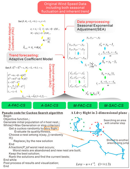
Figure 1. The flowchart of the developed hybrid forecasting models.

• (a) The A-FAC-CS model is the one with additively seasonal exponential adjustment (A), and CS optimizes the first-order adaptive coefficient model (FAC).
• (b) The M-FAC-CS model is the one with multiplicative seasonal exponential adjustment (M), and CS optimizes the first-order adaptive coefficient model (FAC).
• (c) The A-SAC-CS model is the one with additive seasonal exponential adjustment (A), and CS optimizes the second-order adaptive coefficient model (SAC).
• (d) The M-SAC-CS model is the one with multiplicative seasonal exponential adjustment (M), and CS optimizes the second-order adaptive coefficient model (SAC).

4. Simulation Results and Discussion

The daily average wind-speed data is collected from four observation sites of the Xinjiang Uygur Autonomous Region located in northwestern China, including Urumqi City, Korla City, Altay Region and Hami Region. The sample period covers more than four years, from 1 January 2009 to 18 September 2013. The original wind-speed time series of the four observation sites are plotted in Figure 2 together with detailed geographic information.

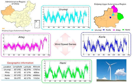
Figure 2. Wind-speed time series and related geographic information.

In Figure 2, the number of the day without unit is in the horizontal axis, while the vertical axis is the wind speed with unit m/s. As we can see from the line charts in Figure 2, for the four observation sites, there are some yearly periodic components in the original wind-speed series. Thus we set the cycle length to be one year by means of direct observation from Figure 2. In particular, original data from 1 January 2009 to 31 December 2012 consisting of four cycles are utilized to calculate the seasonal indices through seasonal exponential adjustment technique as introduced in Section 2.1. In order to validate the effectiveness of the proposed four hybrid forecasting models, daily wind speeds from 1 January 2013 to 31 August 2013 are applied to forecast one day ahead wind-speed data. To facilitate the evaluation and comparison process, the forecast results are summarized according to different forecast months, and two main error criteria are calculated as follows to reflect integral forecasting performance:

$$\mathrm{MAPE}=\frac{1}{N}{\displaystyle \sum }_{i=1}^N\left|\frac{y_i-{\widehat{y}}_i}{y_i}\right|\times 100\%$$

(23)

$$\mathrm{RMSE}=\sqrt{\frac{1}{N}{\displaystyle \sum }_{i=1}^N{\left(y_i-{\widehat{y}}_i\right)}^2}$$

(24)

where $N$ is the forecasting periods number, $y_i$ is the true value at time $i$ and ${\widehat{y}}_i$ is the forecasted value corespondinly.

Next we take Urumqi as the representative example to demonstrate the presented hybrid forecasting methods step by step with intermediary outcomes. In Figure 3, the number of the day without unit is in the horizontal axis, and the vertical axis is the wind speed with unit m/s. As illustrated in Figure 3, the trend series obtained from multiplicative and additive seasonal exponential adjustment are depicted respectively in Figure 3 part A and Figure 3 part B in contrast with the original wind-speed series of Urumqi. In addition, mean values and standard deviations of the above three wind-speed time series are calculated as listed in the table of Figure 3 part D. The vivid line charts and computed results indicate that the seasonal exponential adjustment technique contributes to eliminating periodic fluctuations and lowering standard deviations. That is to say, the trend series are to some extent easier to forecast than the original series.

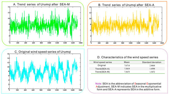
Figure 3. The trend series after seasonal exponential adjustment technique.

4.1. Comparisons of Four Hybrid Models

The parameters of the hybrid models for the cuckoo search algorithm are as follows. There are 25 nests, the step size $\alpha$ is 1, the Lévy flight parameter $\lambda$ is 1.5, the discovery rate of alien eggs $p_a$ is 0.25, and there are 1000 iterations in total. As demonstrated in Figure 4, we plot the forecasting as well as the actual values of Urumqi from January to August in 2013, respectively, under the four developed hybrid forecasting models, namely, A-FAC-CS, A-SAC-CS, M-FAC-CS and M-SAC-CS, as defined in Section 2.3. Moreover, the forecasting errors of the four different forecasting strategies, including both MAPE (mean absolute percentage error) and RMSE (root mean square error) criteria, are also presented in the table of Figure 4. In Figure 4, the number of the day without unit is in the horizontal axis and the vertical axis is the wind speed with unit m/s.

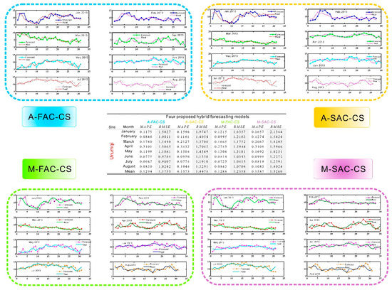
Figure 4. Forecasting results of Urumqi from January to August, 2013.

We can vividly see that the developed hybrid forecasting procedures are capable of achieving satisfactory forecasting performance with respect to the Urumqi observation site. In particular, M-FAC-CS leads to the lowest mean MAPE value of 12.88%, while A-FAC-CS results in the smallest mean RMSE value of 1.1755. Therefore, we can obtain the following conclusion: the first-order adaptive coefficient method performs much better than the second-order adaptive coefficient model, regardless of error criteria, which indicates that higher order algorithms do not necessarily contribute to more desirable forecasting accuracy.

Table 1 lists the forecasting errors of the four kinds of hybrid models, namely A-FAC-CS, A-SAC-CS, M-FAC-CS and M-SAC-CS, from January to August 2013 with respect to four targeted wind-speed observation sites, including Urumqi, Altay, Korla as well as Hami. Moreover, for each observation site, the average MAPE and RMSE values of the eight months are also calculated for each of the presented hybrid forecasting models to reflect and evaluate the overall forecasting performance.

Table 1. Forecast errors of the developed hybrid models.

Site	Month	A-FAC-CS		A-SAC-CS		M-FAC-CS		M-SAC-CS
		MAPE	RMSE	MAPE	RMSE	MAPE	RMSE	MAPE	RMSE
		(%)	(m/s)	(%)	(m/s)	(%)	(m/s)	(%)	(m/s)
Urumqi	Jan.	11.75	1.5027	15.96	1.9747	12.15	1.6357	16.57	2.1344
	Feb.	8.46	1.0811	11.61	1.4054	9.95	1.2163	12.74	1.5424
	Mar.	17.40	1.1440	21.27	1.3706	16.65	1.1752	20.67	1.4205
	Apr.	31.01	1.5065	34.32	1.7042	27.43	1.3948	31.08	1.5966
	May.	11.99	1.1861	15.04	1.4549	13.06	1.3181	16.92	1.6251
	Jun.	7.75	0.9784	9.50	1.1530	8.14	1.0343	9.98	1.2272
	Jul.	6.87	0.9807	7.74	1.1910	7.23	1.0415	8.19	1.2591
	Aug.	8.30	1.0242	10.44	1.3291	8.43	1.0706	10.83	1.4024
	Mean	12.94	1.1755	15.73	1.4478	12.88	1.2358	15.87	1.5260
Altay	Jan.	17.33	1.7730	17.53	1.7924	18.55	1.7958	19.35	1.8774
	Feb.	12.77	1.1273	13.92	1.2158	15.65	1.3816	17.54	1.5096
	Mar.	21.90	1.3127	22.00	1.3170	21.66	1.3692	22.46	1.4189
	Apr.	23.49	1.2979	22.31	1.2727	24.18	1.3401	22.14	1.2667
	May.	13.81	1.2823	14.61	1.3661	13.52	1.2314	14.62	1.3338
	Jun.	6.72	0.7783	6.95	0.8191	8.02	0.9390	9.24	1.0490
	Jul.	6.76	0.7611	6.95	0.7728	8.42	0.9406	8.23	0.9445
	Aug.	7.40	0.7614	9.10	0.9186	9.35	0.9420	9.91	0.9939
	Mean	13.77	1.1367	14.17	1.1843	14.92	1.2425	15.44	1.2992
Korla	Jan.	18.43	1.5578	31.84	2.5856	19.99	1.8015	27.01	2.4067
	Feb.	18.86	1.5369	17.67	1.7954	22.12	1.8093	27.14	2.3944
	Mar.	24.55	1.2167	37.71	1.6057	25.38	1.2436	35.48	1.6143
	Apr.	37.61	1.1623	44.25	1.2791	35.30	1.0951	42.02	1.1497
	May.	17.22	1.5213	22.25	1.9241	19.45	1.7472	22.34	1.9787
	Jun.	8.47	1.0407	13.65	1.6622	9.05	1.1248	14.82	1.6642
	Jul.	9.88	1.2926	12.94	1.6240	10.65	1.4113	12.45	1.5789
	Aug.	9.63	1.0526	15.75	1.6861	9.99	1.0897	13.91	1.5363
	Mean	18.08	1.2976	24.51	1.7703	18.99	1.4153	24.39	1.7904
Hami	Jan.	28.28	1.4712	26.40	1.5940	25.53	1.5595	27.28	1.9086
	Feb.	21.78	1.1774	26.23	1.4843	24.55	1.4277	30.87	1.6943
	Mar.	43.75	1.3477	49.15	1.5802	43.84	1.3548	48.86	1.6425
	Apr.	30.55	1.2230	31.96	1.3845	30.19	1.3349	33.30	1.5001
	May.	11.77	1.5093	14.66	1.9230	14.79	1.9089	18.98	2.5150
	Jun.	10.34	1.2545	11.26	1.4036	11.02	1.3574	12.43	1.6215
	Jul.	10.93	1.5589	14.23	2.0656	11.20	1.5852	14.39	2.0678
	Aug.	15.71	1.9203	16.53	2.0228	16.28	1.9700	17.03	2.0526
	Mean	21.64	1.4328	23.80	1.6823	22.17	1.5623	25.39	1.8753

From Table 1, it can be concluded that for the observation sites of Altay, Korla and Hami, the presented A-FAC-CS forecasting strategy can get the most satisfactory forecasting accuracy. In particular, the mean MAPE and RMSE values of Altay are 13.77% and 1.1367, while for Korla they are 18.08% and 1.2976, respectively. As for Hami, the forecast errors rise slightly to 21.64% and 1.4328. In addition, numerical experiments and simulation results of the four observation sites suggest that the additive seasonal exponential adjustment technique outperforms the multiplicative one when the average forecast errors of the two pairs, namely A-FAC-CS and M-FAC-CS, A-SAC-CS and M-SAC-CS, are compared. Similarly, intensive comparisons of A-FAC-CS and A-SAC-CS in addition to M-FAC-CS and M-SAC-CS indicate that the first-order adaptive coefficient method leads to much more accurate forecasting results than the second-order adaptive coefficient model.

4.2. Compared with Classic Individual Models

In this section, to forecast the daily mean wind speed of the four observation sites as mentioned on Section 3, we also apply four individual models. The models are back propagation (BP) neural network (via Neural Network Toolbox of MATLAB), the autoregressive integrated moving average (ARIMA) model (via Eviews 7), the single first-order adaptive coefficient (FAC) method and the single second-order adaptive coefficient (SAC) method. Those methods are compared with the hybrid model in terms of forecasting ability. Note that the parameters $\beta$ for both FAC and SAC are set as 0.2. The forecast errors of the four conventional approaches are shown in Table 2 with respect to the monthly and average MAPE and RMSE values.

Table 2. Forecast errors of the individual forecasting models.

Site	Month	BP		ARIMA		FAC		SAC
		MAPE	RMSE	MAPE	RMSE	MAPE	RMSE	MAPE	RMSE
		(%)	(m/s)	(%)	(m/s)	(%)	(m/s)	(%)	(m/s)
Urumqi	Jan.	29.18	3.5627	20.98	2.4513	27.90	3.5156	20.58	2.8465
	Feb.	23.75	2.7678	10.87	1.5316	11.14	1.7930	18.04	1.7933
	Mar.	39.43	2.1332	71.11	3.5379	51.44	2.6670	57.09	3.0677
	Apr.	91.88	3.1666	32.62	1.4003	73.91	2.6822	33.24	1.5404
	May.	20.87	2.4769	43.56	4.4628	26.58	2.8222	36.24	3.6641
	Jun.	28.58	3.2256	15.03	1.8523	23.62	2.8243	13.17	1.6420
	Jul.	30.88	3.9388	14.41	2.0055	12.73	1.7973	10.05	1.4265
	Aug.	17.49	2.1202	13.81	1.4732	10.39	1.2257	16.51	1.7810
	Mean	35.26	2.9240	27.80	2.3394	29.71	2.4159	25.62	2.2202
Altay	Jan.	40.43	3.2895	37.19	3.0736	36.33	3.0387	33.90	2.8755
	Feb.	38.38	3.1163	9.59	0.8608	16.99	1.6680	12.13	1.0236
	Mar.	25.38	1.6930	40.31	2.2419	24.70	1.4365	34.39	1.9389
	Apr.	18.40	1.0063	18.64	1.0948	21.30	1.1334	34.28	1.7427
	May.	26.79	2.3141	27.82	2.3983	17.79	1.6172	18.83	1.6681
	Jun.	28.33	2.6634	12.50	1.2670	8.78	1.0173	14.23	1.5739
	Jul.	26.50	2.7111	8.74	1.0413	6.42	0.7566	6.60	0.7798
	Aug.	13.69	1.3585	8.00	0.8084	7.05	0.6831	10.70	1.0428
	Mean	27.24	2.2690	20.35	1.5983	17.42	1.4188	20.63	1.5807
Korla	Jan.	33.98	2.8433	38.10	2.4806	31.82	2.9070	28.30	2.4524
	Feb.	23.81	2.0919	10.15	1.0991	14.44	1.4556	17.79	1.4202
	Mar.	46.62	1.6986	88.11	2.9736	63.89	2.2589	66.56	2.4696
	Apr.	120.12	2.6185	42.88	1.0565	82.55	1.9666	37.12	1.0090
	May.	32.66	3.7806	29.87	3.4455	36.94	3.7943	43.35	4.1106
	Jun.	32.33	3.4578	12.95	1.6919	20.56	2.5124	14.01	1.5748
	Jul.	37.08	4.3698	36.48	4.2827	12.75	1.6153	13.17	1.6535
	Aug.	19.13	2.2059	18.60	1.7018	13.98	1.3956	22.53	2.0864
	Mean	43.22	2.8833	34.64	2.3415	34.62	2.2382	30.35	2.0971
Hami	Jan.	50.96	2.1572	41.63	2.0081	37.87	2.3491	41.12	2.8150
	Feb.	31.59	1.4353	57.07	2.0690	31.78	1.4446	34.35	1.5961
	Mar.	95.89	2.1456	54.76	1.4215	75.49	1.7488	89.69	2.0288
	Apr.	33.35	1.3148	55.19	2.8800	50.70	2.0461	55.29	2.0860
	May.	57.16	5.8094	31.80	3.4077	37.40	4.1542	25.85	3.2662
	Jun.	47.21	5.3752	14.45	1.8675	17.78	2.0651	14.55	1.8092
	Jul.	37.52	4.3132	12.15	1.6135	8.75	1.2439	8.75	1.2199
	Aug.	25.37	2.9380	19.59	2.1095	14.50	1.5831	17.68	1.9387
	Mean	47.38	3.1861	35.83	2.1721	34.28	2.0794	35.91	2.0950

As shown in Table 2, the mean MAPE values of the BP neural network regarding the four observation sites, namely Urumqi, Altay, Korla as well as Hami, are 35.26%, 27.24%, 43.22% and 47.38%, respectively, while the average RMSE values of the ARIMA model are 2.3394, 1.5983, 2.3415 and 2.1721. In addition, the BP neural network and the ARIMA model yield extremely high forecast errors for some months. For example, the MAPE value of the BP neural network with respect to Urumqi in April is as high as 91.88% and the MAPE value of the ARIMA model with respect to Korla in March reaches up to 88.11%. Apparently, these extremely inaccurate forecasting results have an adverse effect on wind farm operations and may threaten the security of the grid when wind power is integrated for electricity supply. Thus, it is highly significant to propose novel hybrid forecasting strategies to replace the individual forecasting models in practice and achieve desirable forecasting accuracy.

To better illustrate the superiority of the hybrid forecasting approaches presented in this paper, we list the mean MAPE values from January to August in 2013 obtained from the four individual forecasting models as well as one hybrid forecasting strategy in Table 3. Note that there is no harm in selecting the specific hybrid model with the maximal MAPE value among the four kinds of developed hybrid methods to represent the hybrid forecasting models in the last column of Table 3.

Table 3. The mean MAPE values (%) of different forecasting models.

Site	BP	ARIMA	FAC	SAC	Hybrid
Urumqi	35.26	27.80	29.71	25.62	15.87
Altay	27.24	20.35	17.42	20.63	15.44
Korla	43.22	34.64	34.62	30.35	24.51
Hami	47.38	35.83	34.28	35.91	25.39

As we can clearly see from Table 3, the presented hybrid forecasting models can remarkably reduce forecasting errors compared with conventional methods. Taking Urumqi as an example, through simple calculation we find the mean MAPE value using the hybrid model decrease by 19.39%, 11.93%, 13.84% and 7.75% compared to the BP neural network, ARIMA, FAC and SAC models, respectively. Similar results can be made based on the forecast results of other three observation sites as illustrated in Table 3. To sum up, the novel hybrid forecasting strategies developed in this paper are effective, which is proven by a number of numerical simulations whose results are listed in Table 1 and Table 2. Furthermore, the innovative hybrid models make significant improvements to traditional single forecasting approaches and provide more satisfactory forecasting accuracy for practical applications in wind power generation and grid regulation.

Next, to verify the significance of the parameter optimization process in the hybrid forecasting strategies, we construct four kinds of forecasting approaches using the seasonal exponential adjustment technique and the adaptive coefficient methods whose exogenous parameters $\beta$ are predetermined (with the value 0.2) in the conventional way rather than being optimized by the cuckoo search algorithm. These four kinds of methods are denoted as A-FAC, A-SAC, M-FAC and M-SAC, respectively, corresponding to their counterparts A-FAC-CS, A-SAC-CS, M-FAC-CS and M-SAC-CS with optimal parameters attained from the cuckoo search algorithm, respectively. Furthermore, their forecast errors are summarized in Table 4.

Table 4. Forecast errors of the hybrid models with predetermined parameters.

Site	Month	A-FAC		A-SAC		M-FAC		M-SAC
		MAPE	RMSE	MAPE	RMSE	MAPE	RMSE	MAPE	RMSE
		(%)	(m/s)	(%)	(m/s)	(%)	(m/s)	(%)	(m/s)
Urumqi	Jan.	22.80	2.9656	21.07	2.9327	23.28	3.0388	20.62	2.9587
	Feb.	11.15	1.7389	10.96	1.4012	11.82	1.8162	11.54	1.4282
	Mar.	37.45	2.0957	46.76	2.5729	37.19	2.1349	46.36	2.6037
	Apr.	52.60	1.9398	36.64	1.6318	50.31	1.8568	37.08	1.5703
	May.	23.06	2.3548	27.38	2.6666	23.92	2.4360	28.64	2.7845
	Jun.	10.98	1.3755	9.88	1.3285	11.18	1.4089	10.12	1.3996
	Jul.	10.84	1.5237	10.95	1.5242	11.08	1.5498	11.75	1.6018
	Aug.	11.98	1.4231	14.06	1.5589	12.23	1.4573	13.81	1.5609
	Mean	22.61	1.9272	22.21	1.9521	22.63	1.9624	22.49	1.9885
Altay	Jan.	28.72	2.5901	25.89	2.3687	28.86	2.6122	25.27	2.3484
	Feb.	14.60	1.3839	14.33	1.2246	15.99	1.5160	17.63	1.5045
	Mar.	20.51	1.2551	25.87	1.5205	20.39	1.2970	24.29	1.5199
	Apr.	23.46	1.2831	33.06	1.7122	24.50	1.3507	33.76	1.7828
	May.	13.78	1.2706	14.66	1.3391	12.72	1.1755	12.54	1.1700
	Jun.	7.14	0.8500	10.37	1.1788	7.99	0.9452	9.25	1.0982
	Jul.	7.08	0.7932	7.00	0.7880	8.27	0.9380	8.36	0.9621
	Aug.	7.66	0.7769	8.83	0.8922	9.33	0.9381	9.43	0.9508
	Mean	15.37	1.2754	17.50	1.3780	16.01	1.3466	17.57	1.4171
Korla	Jan.	33.06	2.8499	31.46	2.8438	33.21	2.8740	29.64	2.7286
	Feb.	19.06	1.8813	16.62	1.5586	19.42	1.9041	19.24	1.7313
	Mar.	43.74	1.7817	56.44	2.2029	45.87	1.9322	57.89	2.3821
	Apr.	59.00	1.4235	44.51	1.2460	56.58	1.3678	43.84	1.1604
	May.	33.43	3.2072	38.10	3.3685	36.05	3.3229	42.31	3.5991
	Jun.	12.63	1.4397	12.99	1.5012	13.54	1.5625	15.78	1.8073
	Jul.	14.50	1.8615	15.50	1.8892	16.29	2.0008	18.80	2.1764
	Aug.	15.23	1.4691	16.23	1.5660	16.30	1.5598	17.46	1.6847
	Mean	28.91	1.9892	28.98	2.0220	29.66	2.0655	30.62	2.1587
Hami	Jan.	51.74	2.5343	53.81	2.5421	51.74	2.5154	53.76	2.5358
	Feb.	31.79	1.7927	32.06	1.6615	31.75	1.7633	34.41	1.7066
	Mar.	52.34	1.3813	62.86	1.5416	54.02	1.4182	63.92	1.5989
	Apr.	44.74	1.7330	47.42	1.7181	45.23	1.7231	46.41	1.7271
	May.	17.44	2.2514	18.67	2.3539	17.80	2.2329	19.55	2.4045
	Jun.	14.90	1.8122	16.21	1.9865	16.61	2.0506	19.64	2.4182
	Jul.	11.14	1.4544	13.32	1.7891	12.80	1.7177	18.10	2.4109
	Aug.	15.78	1.7640	16.29	1.7779	16.69	1.8476	16.97	1.8529
	Mean	29.98	1.8404	32.58	1.9213	30.83	1.9086	34.09	2.0818

To vividly illustrate the improved forecasting accuracy that is attributable to optimal parameter selection, we put the mean MAPE values of hybrid models integrated with and without the cuckoo search algorithm together in Table 5 for the four observation sites, namely Urumqi, Altay, Korla and Hami.

Table 5. The mean MAPE values (%) of hybrid models with and without the CS algorithm.

Model	Urumqi	Altay	Korla	Hami
A-FAC	22.61	15.37	28.91	29.98
A-FAC-CS	12.94	13.77	18.08	21.64
A-SAC	22.21	17.50	28.98	32.58
A-SAC-CS	15.73	14.17	24.51	23.80
M-FAC	22.63	16.01	29.66	30.83
M-FAC-CS	12.88	14.92	18.99	22.17
M-SAC	22.49	17.57	30.62	34.09
M-SAC-CS	15.87	15.44	24.39	25.39

As shown in Table 5, compared with hybrid forecasting strategies based on seasonal exponential adjustment techniques and adaptive coefficient methods with predetermined parameters, the further integrated cuckoo search algorithm contributes markedly to decreasing forecast errors. In particular, for Urumqi, the mean MAPE values of the eight months are reduced by 9.67%, 6.48%, 9.75% and 6.62% after the cuckoo search algorithm is introduced to the hybrid models, compared with A-FAC-CS, A-SAC-CS, M-FAC-CS and M-SAC-CS, respectively. The comparisons of the forecast results regarding other three observation sites also indicate similar patterns, as shown in Table 5. Consequently, it can be concluded that the parameter optimization process should be regarded as a requisite component in the constructed hybrid forecast model. Moreover, the cuckoo search algorithm is a powerful search engine for parameters of the adaptive coefficient methods, and it is capable of improving forecast accuracy.

5. Conclusions

This paper presents four novel kinds of hybrid models based on the seasonal exponential adjustment in the multiplicative or additive form, the first- or second-order adaptive coefficient methods and the cuckoo search algorithm for wind-speed forecasting. These models are significant because accurate wind-speed forecasting supplies essential information for wind-power assessment, wind-farm operations, integrated grid management and so on. To examine the effectiveness and superiority of the hybrid approaches proposed in this paper, daily mean wind-speed data sampled from four observation sites in Xinjiang Uygur Autonomous Region of China are taken into investigation. The simulation results described in Section 4 indicate that the developed innovative hybrid strategies provide satisfactory forecast accuracy.

As demonstrated in Section 4.1, there is sufficient evidence to show that the proposed hybrid models perform much better than existing individual forecasting approaches, such as the BP neural network, the ARIMA and the single adaptive coefficient method. Moreover, numerical experiments also suggest that introducing the CS algorithm to the hybrid forecasting methods is highly recommended because it contributes remarkably to improving forecasting accuracy compared with the hybrid models using predetermined parameters.

We contribute to existing forecast model research by innovatively constructing hybrid forecasting models and integrating conventional adaptive coefficient models with an advanced cuckoo search algorithm. In particular, seasonal components and inherent trends are processed separately, which is regarded as an important data preprocessing technique in our research. In addition, the performance of the adaptive coefficient models is further improved by our work since we introduce the cuckoo search algorithm to conduct parameter optimization.

To sum up, considering their effectiveness and accuracy, the proposed hybrid forecasting strategies could be applied at large-scale wind farms to accomplish regular forecasting work. In addition, the proposed hybrid models for wind-speed forecasting also shed light on existing forecasting approaches for other variables, such as electricity demand and stock prices.

References

- Tomczewski, A.; Kasprzyk, L.; Nadolny, Z. Reduction of Power Production Costs in a Wind Power Plant–Flywheel Energy Storage System Arrangement. Energies 2019, 12, 1942. [Google Scholar] [CrossRef]
- Zhang, W.; Wu, J.; Wang, J.; Zhao, W.; Shen, L. Performance analysis of four modified approaches for wind speed forecasting. Appl. Energy 2012, 99, 324–333. [Google Scholar] [CrossRef]
- Zhao, Y.; Ye, L.; Li, Z.; Song, X.; Lang, Y.; Su, J. A novel bidirectional mechanism based on time series model for wind power forecasting. Appl. Energy 2016, 177, 793–803. [Google Scholar] [CrossRef]
- Liu, H.; Mi, X.; Li, Y. Smart multi-step deep learning model for wind speed forecasting based on variational mode decomposition, singular spectrum analysis, LSTM network and ELM. Energy Convers. Manag. 2018, 159, 54–64. [Google Scholar] [CrossRef]
- Qiu, X.; Zhang, L.; Suganthan, P.N.; Amaratunga, G.A. Oblique random forest ensemble via Least Square Estimation for time series forecasting. Inf. Sci. 2017, 420, 249–262. [Google Scholar] [CrossRef]
- Ren, Y.; Suganthan, P.; Srikanth, N.; Amaratunga, G.; Suganthan, P. Random vector functional link network for short-term electricity load demand forecasting. Inf. Sci. 2016, 367, 1078–1093. [Google Scholar] [CrossRef]
- Louka, P.; Galanis, G.; Siebert, N.; Kariniotakis, G.; Katsafados, P.; Pytharoulis, I.; Kallos, G. Improvements in wind speed forecasts for wind power prediction purposes using Kalman filtering. J. Wind Eng. Ind. Aerodyn. 2008, 96, 2348–2362. [Google Scholar] [CrossRef]
- Wang, Y.; Hu, Q.; Meng, D.; Zhu, P. Deterministic and probabilistic wind power forecasting using a variational Bayesian-based adaptive robust multi-kernel regression model. Appl. Energy 2017, 208, 1097–1112. [Google Scholar] [CrossRef]
- An, S.; Shi, H.; Hu, Q.; Li, X.; Dang, J. Fuzzy rough regression with application to wind speed prediction. Inf. Sci. 2014, 282, 388–400. [Google Scholar] [CrossRef]
- Wang, S.; Zhang, N.; Wu, L.; Wang, Y. Wind speed forecasting based on the hybrid ensemble empirical mode decomposition and GA-BP neural network method. Renew. Energy 2016, 94, 629–636. [Google Scholar] [CrossRef]
- Han, Q.; Wu, H.; Hu, T.; Chu, F. Short-Term Wind Speed Forecasting Based on Signal Decomposing Algorithm and Hybrid Linear/Nonlinear Models. Energies 2018, 11, 2976. [Google Scholar] [CrossRef]
- Huang, Y.; Yang, L.; Liu, S.; Wang, G. Multi-Step Wind Speed Forecasting Based On Ensemble Empirical Mode Decomposition, Long Short Term Memory Network and Error Correction Strategy. Energies 2019, 12, 1822. [Google Scholar] [CrossRef]
- Sun, S.; Wei, L.; Xu, J.; Jin, Z. A New Wind Speed Forecasting Modeling Strategy Using Two-Stage Decomposition, Feature Selection and DAWNN. Energies 2019, 12, 334. [Google Scholar] [CrossRef]
- Blanchard, T.; Samanta, B. Wind Speed Forecasting Using Neural Networks. Wind Eng. 2019. Available online: https://doi.org/10.1177/0309524X19849846 (accessed on 23 September 2019).
- Chitsazan, M.A.; Fadali, M.S.; Trzynadlowski, A.M. Wind speed and wind direction forecasting using echo state network with nonlinear functions. Renew. Energy 2019, 131, 879–889. [Google Scholar] [CrossRef]
- Zhou, Q.; Wang, C.; Zhang, G. Hybrid forecasting system based on an optimal model selection strategy for different wind speed forecasting problems. Appl. Energy 2019, 250, 1559–1580. [Google Scholar] [CrossRef]
- Hu, J.; Wang, J.; Zeng, G. A hybrid forecasting approach applied to wind speed time series. Renew. Energy 2013, 60, 185–194. [Google Scholar] [CrossRef]
- Fu, W.; Wang, K.; Li, C.; Tan, J. Multi-step short-term wind speed forecasting approach based on multi-scale dominant ingredient chaotic analysis, improved hybrid GWO-SCA optimization and ELM. Energy Convers. Manag. 2019, 187, 356–377. [Google Scholar] [CrossRef]
- Zhang, Z.; Qin, H.; Liu, Y.; Yao, L.; Yu, X.; Lu, J.; Jiang, Z.; Feng, Z. Wind speed forecasting based on Quantile Regression Minimal Gated Memory Network and Kernel Density Estimation. Energy Convers. Manag. 2019, 196, 1395–1409. [Google Scholar] [CrossRef]
- Li, Y.; Shi, H.; Han, F.; Duan, Z.; Liu, H. Smart wind speed forecasting approach using various boosting algorithms, big multi-step forecasting strategy. Renew. Energy 2019, 135, 540–553. [Google Scholar] [CrossRef]
- Wu, Y.-X.; Wu, Q.-B.; Zhu, J.-Q. Data-driven wind speed forecasting using deep feature extraction and LSTM. IET Renew. Power Gener. 2019, 13, 2062–2069. [Google Scholar] [CrossRef]
- Cassola, F.; Burlando, M. Wind speed and wind energy forecast through Kalman filtering of Numerical Weather Prediction model output. Appl. Energy 2012, 99, 154–166. [Google Scholar] [CrossRef]
- Niu, X.; Wang, J. A combined model based on data preprocessing strategy and multi-objective optimization algorithm for short-term wind speed forecasting. Appl. Energy 2019, 241, 519–539. [Google Scholar] [CrossRef]
- Chen, K.; Yu, J. Short-term wind speed prediction using an unscented Kalman filter based state-space support vector regression approach. Appl. Energy 2014, 113, 690–705. [Google Scholar] [CrossRef]
- Guo, Z.; Wu, J.; Lu, H.; Wang, J.Z. A case study on a hybrid wind speed forecasting method using BP neural network. Knowl.-Based Syst. 2011, 24, 1048–1056. [Google Scholar] [CrossRef]
- Zhu, S.; Wang, J.; Zhao, W.; Wang, J. A seasonal hybrid procedure for electricity demand forecasting in China. Appl. Energy 2011, 88, 3807–3815. [Google Scholar] [CrossRef]
- Cadenas, E.; Jaramillo, O.A.; Rivera, W. Analysis and forecasting of wind velocity in chetumal, quintana roo, using the single exponential smoothing method. Renew. Energy 2010, 35, 925–930. [Google Scholar] [CrossRef]
- De Faria, E.; Albuquerque, M.P.; González, J.; Cavalcante, J.; Albuquerque, M.P. Predicting the Brazilian stock market through neural networks and adaptive exponential smoothing methods. Expert Syst. Appl. 2009, 36, 12506–12509. [Google Scholar] [CrossRef]
- Yang, X.S.; Deb, S. Cuckoo search via Lévy flights. In Proceedings of the World Congress on Nature and Biologically Inspired Computing (NaBIC), Coimbatore, India, 9–11 December 2009. [Google Scholar]
- Yang, X.S. Nature-Inspired Metaheuristic Algorithms, 2nd ed.; Luniver Press: Frome, UK, 2010. [Google Scholar]
- Yang, X.S.; Deb, S. Multiobjective cuckoo search for design optimization. Comput. Oper. Res. 2013, 40, 1616–1624. [Google Scholar] [CrossRef]
© 2019 by the authors. Licensee MDPI, Basel, Switzerland. This article is an open access article distributed under the terms and conditions of the Creative Commons Attribution (CC BY) license (http://creativecommons.org/licenses/by/4.0/).