Axisymmetric Numerical Investigation on Steam Bubble Condensation

Abstract

In order to obtain a high-accuracy and adaptable condensation phase change model, this paper selects the Nusselt number correlation formula that Kim proposed based on the experimental data and adjusts the Nusselt number in the bubble condensation process by calculating the phase change coefficient of the Lee model in the UDF. Through the simulation and fine-tuning of the 12 groups of operating conditions, the formula for the change of the phase change coefficient of the Lee model during the bubble condensation process is obtained. The accuracy and wide applicability of the variation formula are verified by comparison with various types of experimental data. The Lee model provides a certain reference for the numerical simulation of the bubble condensation process. The numerical simulation of the condensation process of vapor bubbles is carried out by using the formula of the phase change coefficient. The error between the simulation result of the bubble volume change and the experimental result is lower than ±15%, which basically verified the reliability of the numerical model adopted in this study. The bubble condensation process has been analyzed under various operating conditions. The simulation results show that when the bubble rises, disturbance occurs with the fluid and several tiny eddies are generated on the side of the bubble. Micro-circulation of the vapor inside the bubble accelerates the heat and mass transfer rate at the gas–liquid interface. When condensation occurs, the mass transfer rate at the interface is different and the pressure inside the bubble is higher than that around it.

1. Introduction

The steam bubble condensation is a classical direct contact condensation (DDC) and it is a typical part of heat transfer, which is widely encountered in the industrial field, especially electronic cooling and nuclear reactor. Due to several factors that affect the process of bubble condensation and its complicated mechanism, many attentions have been attracted on this topic in the past decades.

In order to acquire regulations of steam bubble in subcooled water, researchers have performed various experiments [1,2,3,4]. Kamei and Hirata [5] recorded the process of vapor bubble condensation in subcooled water with a high-speed camera. They studied the effect of different pressures, temperatures, and initial diameters for bubble condensation, based on a frame-by-frame analysis. It provides a good experimental comparison for future investigation. In Kim and Park’s experiments [6], interfacial heat transfer coefficient is correlated at low pressure in subcooled boiling flow and the bubble condensation rate is derived by orthogonal, two-image processing. Issa et al. [7] investigated steam bubbles condensation injected into a DN100 vertical pipe with flowing low-subcooled water and a new Nu–Re correlation is developed. Nguyen et al. [8] proposed a new measurement of the condensation rate which is different from previous methods based on optical visualization. Two ultrasonic frequencies were used to measure the velocity distribution of bubble surface along two measuring lines in subcooled boiling.

Comparing with experiments, numerical simulation method could get more information on the behavior of bubble condensation [9,10,11]. The condensation behavior of a vapor bubble in subcooled water was calculated with Moving Particle Semi-implicit (MPS) method by Tian et al. [12]. Using the Volume of Fluid (VOF) multiphase flow model, Pan et al. [13] simulated single vapor bubble condensation behaviors in subcooled boiling flow in two different vertical rectangular channels. A mass and energy transfer model of the bubble condensing process caused by the interfacial heat transfer is developed to describe the transport of two-phase interface. Liu et al. [14] used the VOF method to establish a computational fluid dynamics (CFD) model of multi-bubble condensation. Owoeye and Schubring [15] analyzed a single bubble behaviors in upward subcooled flo w boiling with VOF model and large eddy simulation (LES) turbulence model. Bahreini et al. [16] tracked the phase interface via the VOF method with continuous surface force (CSF) model, carried out in the open source OpenFOAM CFD package. Meanwhile, they modified the original energy equation and mass transfer model for phase change and developed a new solver. Samkhaniani and Ansari [17,18] simulated subcooled boiling with color function volume of fluid (CF-VOF) method. A smoothing filter is implemented to improve the curvature calculation for the sake of reducing the stray current near interface. The research reveals some basic characteristics of single bubble condensation and multi bubble condensation, which is of guiding significance for further application..

Nowadays, there are a large number of experimental and numerical investigations on bubble condensation with various numerical software and phase change models [19,20]. While, most of them, to ensure the change of bubble volume consistent with experimental correlation, calculate the current bubble condensation firstly, then the average heat and mass transfer at the bubble interface is obtained by calculating the bubble surface area. Therefore, heat and mass transfer at the interface is the same in any circumstances, which is not in line with the actual situation. In order to obtain a high-accuracy and adaptable condensation model, the Lee phase change model is improved to simulate the bubble condensation process. It is a common way to simulate the condensation process using the Lee model, but the phase change coefficients of the model are often different in cases. To determine the phase change coefficient in different conditions, it is necessary to adjust the phase change coefficient in time according to the actual process of bubble condensation. The bubble condensation process under different operating conditions is simulated in this paper based on the Nusselt number correlation proposed by Kim. For the process, the phase change coefficient is adjusted by Proportion Integral Differential (PID) algorithm to obtain the value of phase change coefficient in different condensation stages, and the formula of phase change coefficient is obtained after correlated. The accuracy and wide applicability of the variation formula are verified by comparison with various types of experimental data. The Lee model provides a certain reference for the numerical simulation of bubble condensation process. The numerical simulation of the condensation process of vapor bubbles is carried out by using the formula of phase change coefficient.

2. Numerical Methodology

2.1. Governing Equations

In this paper, the liquid and vapor are set as the first and second phases respectively. ANSYS Fluent (Release 15.0, ANSYS Inc, Canonsburg, PA, USA) realizes tracking the interface between the phases by solving the continuity of volume fraction of a phase:

$$\frac{1}{\partial t}[\frac{\partial }{\partial t}({\alpha }_q{\rho }_q)+\nabla ·({\alpha }_q{\rho }_q{\overrightarrow{v}}_q)=+{\sum }_{p=1}^n({\dot{m}}_{pq}-{\dot{m}}_{qp})],$$

(1)

where ${\dot{m}}_{qp}$ expresses the mass transfer from the q-phase fluid to the p-phase fluid. ${\dot{m}}_{pq}$ is the mass transfer from the p-phase fluid to the q-phase fluid.

The velocity field is obtained by solving a set of momentum equations in all computational domains and is based on all phase fluids:

$$\frac{\partial }{\partial t}\left(\rho \overrightarrow{v}\right)+\nabla ·\left(\rho \overrightarrow{v}\overrightarrow{v}\right)=-\nabla p+\nabla ·\left[\mu \left(\nabla \overrightarrow{v}+\nabla {\overrightarrow{v}}^T\right)\right]+\rho \overrightarrow{g}+\overrightarrow{F}.$$

(2)

The energy equation is also based on all phase fluids:

$$\frac{\partial }{\partial t}\left(\rho E\right)+\nabla ·\left(\overrightarrow{v}\left(\rho E+p\right)\right)=\nabla ·\left(k_{eff}\nabla T\right)+S_h.$$

(3)

Here, $S_h$ is source item, including radiation and other volume heat sources.

2.2. Interfacial Surface Tension Model

Surface tension is the result of molecular attraction in fluids. This study adopts the CSF model which results in the addition of surface tension to the momentum equation in VOF calculation. The pressure difference across the surface is dependent on $\sigma$ and the radius of curvature $R_1$ and $R_2$ in two orthogonal directions:

$$p_1-p_2=\sigma \left(\frac{1}{R_1}+\frac{1}{R_2}\right).$$

(4)

In continuous surface tension model, the normal vector on an interface is obtained by the gradient of phase friction. ${\alpha }_q$ as volume friction of the $q^{th}$ phase:

$$n=\nabla {\alpha }_q.$$

(5)

The curvature $k$ is represented by $\hat{n}$ the (divergence of the unit normal) as

$$k=\nabla ·\frac{\hat{n}}{\left|n\right|}$$

(6)

According to the divergence theorem, the force at the surface can be converted into a volume force, which is the increased source term in the momentum equation:

$$F_{vol}={\sum }_{pairsij,i<j}{\sigma }_{ij}\frac{{\alpha }_i{\rho }_i{k}_j\nabla {\alpha }_j+{\alpha }_j{\rho }_j{k}_i\nabla {\alpha }_i}{\frac{1}{2}\left({\rho }_i+{\rho }_j\right)}.$$

(7)

To prevent two phases from presenting in an interfacial cell, $k_i=-k_j$ and $\nabla {\alpha }_i=-\nabla {\alpha }_j$, Equation (7) can be simplified as:

$$F_{vol}={\sigma }_{ij}\frac{\rho k_i\nabla {\alpha }_i}{\frac{1}{2}\left({\rho }_i+{\rho }_j\right)}.$$

(8)

2.3. Heat and Mass Transfer Model

The Lee model is a phase change model based on physical basis, where the liquid–vapor mass transfer (evaporation and condensation) process is controlled by the gas transfer equation:

$$\frac{\partial }{\partial t}\left({\alpha }_v{\rho }_v\right)+\nabla ·\left({\alpha }_v{\rho }_v{\overrightarrow{V}}_v\right)={\dot{m}}_{lv}-{\dot{m}}_{vl}.$$

(9)

In the above equation, the subscript v is the gas phase. ${\alpha }_v$ expresses the volume fraction of gas phase. ${\rho }_v$ presents the density of gas phase. ${\overrightarrow{V}}_v$ is the velocity of gas phase. ${\dot{m}}_{lv}$ and ${\dot{m}}_{vl}$ present the mass transfer rate of evaporation and condensation, respectively.

Fluent defines forward mass transfer as the evaporation-condensation process from liquid to steam. Based on different temperature, mass transfer model can be described as:

If $T_l>T_{sat}$ (evaporation):

$${\dot{m}}_{lv}=coeff\ast {\alpha }_l{\rho }_l\frac{\left(T_l-T_{sat}\right)}{T_{sat}}.$$

(10)

If $T_v<T_{sat}$ (condensation):

$${\dot{m}}_{vl}=coeff\ast {\alpha }_v{\rho }_v\frac{\left(T_{sat}-T_v\right)}{T_{sat}}.$$

(11)

coeff is phase change coefficient. The phase change coefficient would get different values with different conditions, which is also called the relaxation time.

According to Hertz Knudsen formula, evaporation-condensation flow rate is obtained based on the theory of interface dynamics:

$$\mathrm{F}=\mathsf{\beta }\sqrt{\frac{M}{2\pi R{T}_{sat}}}\left(P^{*}-P_{sat}\right).$$

(12)

Here, $\mathsf{\beta }$ is adjustment coefficient, which expresses the part of vapor molecules that enter liquid and are absorbed. $P^{*}$ is the partial pressure of the gas phase on the gas side. Clapeyron-Clausius equation associates pressure with temperature under saturation conditions:

$$\frac{dP}{dT}=\frac{L}{T\left(v_v-v_l\right)}.$$

(13)

$v_v$ and $v_v$ are the reciprocal of the density of the vapor and liquid, respectively.

When $P^{*}$ and $T^{*}$ close to saturation, Clapeyron–Clausius can be written as:

$$P^{*}-P_{sat}=\frac{L}{T\left(v_v-v_l\right)}\left(T^{*}-T_{sat}\right).$$

(14)

Substitute (14) into (12):

$$\mathrm{F}=\mathsf{\beta }\sqrt{\frac{M}{2\pi R{T}_{sat}}}L\left(\frac{{\rho }_v{\rho }_l}{{\rho }_l-{\rho }_v}\right)\frac{\left(T^{*}-T_{sat}\right)}{T_{sat}}.$$

(15)

β approaches 1.0 at close equilibrium.

If all bubbles are assumed to have the same diameter, the interfacial area density is:

$$A_i=\frac{6{\alpha }_v{\alpha }_l}{d_b}.$$

(16)

$d_b$ is the average diameter of the discrete bubbles. The mass source term can be expressed as:

$$\mathrm{F}{A}_i=\frac{6}{d_b}\beta \sqrt{\frac{M}{2\pi R{T}_{sat}}}L\left(\frac{{\alpha }_v{\rho }_v}{{\rho }_l-{\rho }_v}\right)\left[{\alpha }_l{\rho }_l\frac{\left(T^{*}-T_{sat}\right)}{T_{sat}}\right].$$

(17)

Therefore, the coeff can be defined as:

$$coeff=\frac{6}{d_b}\beta \sqrt{\frac{M}{2\pi R{T}_{sat}}}L\left(\frac{{\alpha }_v{\rho }_v}{{\rho }_l-{\rho }_v}\right).$$

(18)

As can be seen from (18), the calculation of the Lee model not only needs to obtain the temperature, physical properties, and phase volume fraction of the grid element, but also needs to define the coefficient coeff. Since it is difficult to determine the coeff, its value is often regarded as an empirical constant in practice (0.1~$5 \times {10}^6$).

2.4. Coeff Correlation with Numerical Method

In order to obtain a high-accuracy and adaptable condensation phase change model, this paper selects the Nusselt number correlation that Kim summarized based on the experimental data and adjusts the Nusselt number in the bubble condensation process by calculating the phase change coefficient of the Lee model in the UDF. The PID algorithm is adopted to adjust the coeff slightly. By compiling UDF, the coeff is changed in time to make the Nusselt number in line with the correlation.

The Nusselt number correlation formula:

$$N{u}_c=0.2575R{e}_b^{0.7}P{r}^{-0.4564}J{a}^{0.2043}.$$

(19)

The PID algorithm:

$$∆u\left(k\right)=A·e\left(k\right)-B·e\left(k-1\right)+C·e\left(k-2\right).$$

(20)

In this study, we choose 12 groups of operating conditions to simulate.

Based on the numerical result of the 12 groups of operating conditions, the formula for the change of the phase change coefficient of the Lee model during the bubble condensation process is obtained.

$$coeff=-2266+7626v_b^{0.4528}{D}_b^{-0.366}$$

(21)

The diameter and average velocity of the bubble are defined as follows:

$$D_b=\sqrt[3]{\frac{6V_b}{\pi }}$$

(22)

$$v_b=\frac{{\sum }_i{v}_{g,i}{\rho }_{g,i}{\alpha }_{g,i}{V}_i}{{\sum }_i{\rho }_{g,i}{\alpha }_{g,i}{V}_i},$$

(23)

where i expresses the grid number of the calculation domain. ${\alpha }_{g,i}$ is gas volume fraction. $V_i$ is the volume of the grid cell. ${\rho }_{g,i}$ is the density of gas phase. $v_{g,i}$ represents the velocity of gas phase in the grid cell.

Relevant criterion numbers are defined as:

$$Re=\frac{{\rho }_w{v}_b{D}_b}{{\mu }_w},$$

(24)

$$Pr=\frac{v_w}{{\alpha }_w},$$

(25)

$$Ja=\frac{{\rho }_w{C}_{pw}∆T}{{\rho }_b\left(h_s-h_w\right)},$$

(26)

$$Nu=\frac{h{D}_b}{{\lambda }_w}.$$

(27)

To calculate the actual heat transfer coefficient, insert the mass change fraction ∆M into the following equation:

$$h=\frac{∆M\left(h_s-h_w\right)}{A_b\left(T_b-T_w\right)}.$$

(28)

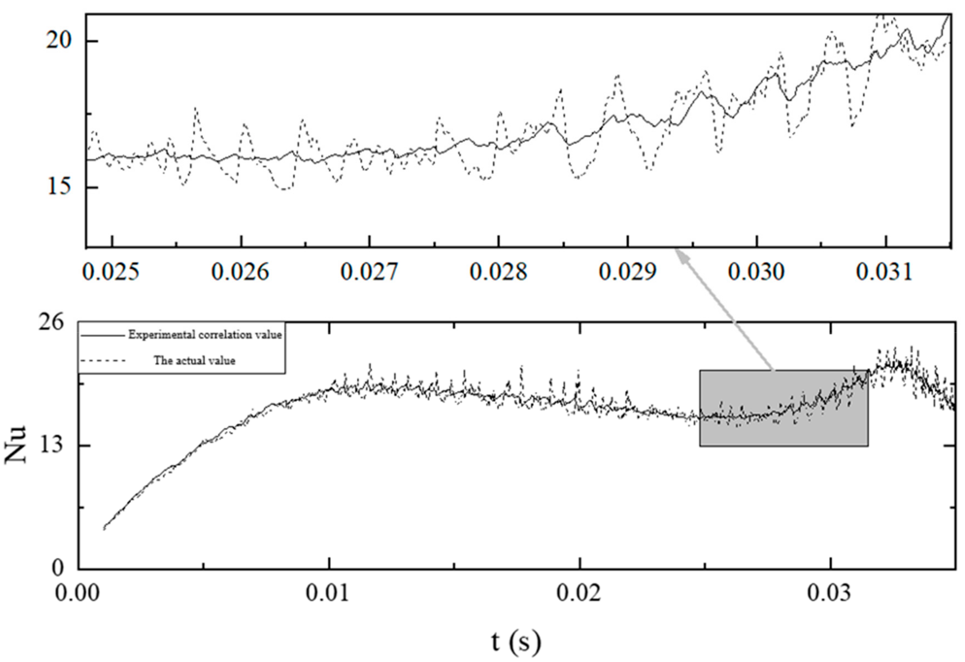
Figure 1 shows the Nu number in the simulation result moves up and down in the Nu number calculated by Kim’s empirical correlation, which means the phase change coefficient adjusted by PID controller can be consistent with the data of correlation calculation in bubble condensation process.

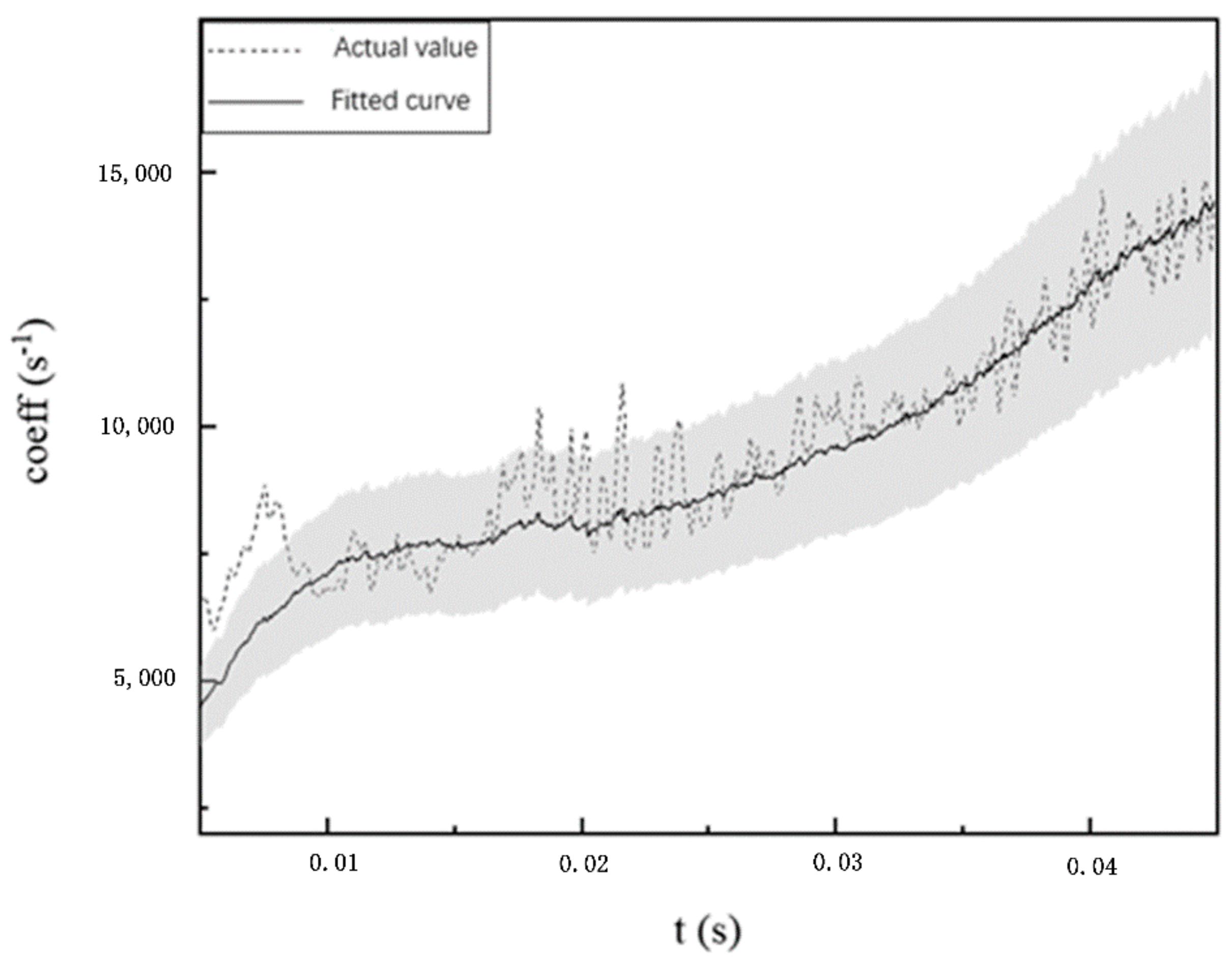
Figure 2 shows the fitting correlation curve and the change of coeff value in the simulation process in the working condition 2 in

Table 1. The condition of simulation.

Sequence Number	Degree of Supercooling (°C)	Initial Diameter (mm)
1 2 3	10	3 5 7
4 5 6	15	3 5 7
7 8 9	20	3 5 7
10 11 12	25	3 5 7

. It can be seen that the actual coeff value adjusted by PID oscillates around the curve of fitting Formula (21), but the fluctuation does not exceed 20% within the error range.

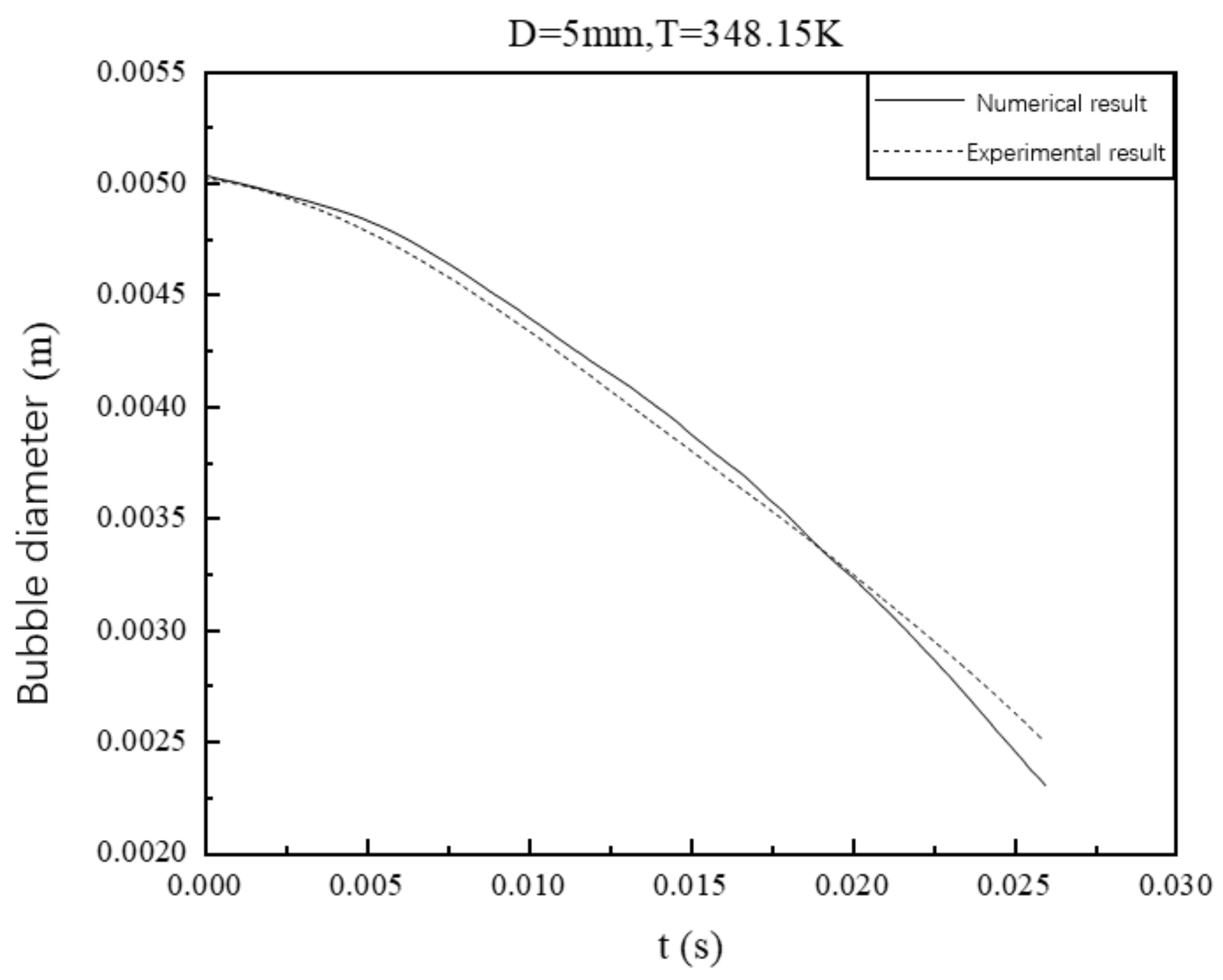
Formula (21) is inserted into Lee’s phase change model and numerical simulation is carried out for working condition 11 in Table 1. The variation of bubble diameter in the condensation process is compared with Kim’s experimental results. As can be seen from the Figure 3, the solid line and the dotted line represent the bubble diameter of simulation and experiment, respectively. The two lines almost coincide initially, and they start to diverge at 0.004 s. The dotted line decreases faster, below the solid line. At 0.19 s, the two lines crossed again, the slope of the solid line gets larger, and the dotted line is above. The deviation between the two lines began to increase, but the maximum deviation value is also very small, less than 0.2 mm. Therefore, it can be considered that the numerical result is in accordance with the experimental result, and Formula (21) can be applied to calculate phase change coefficient during the bubble condensation process.

3. Computational Domain and Boundary Conditions

To reduce the calculation time and improve the calculation efficiency, this paper assumes that the rising process of the bubble is a two-dimensional axisymmetric process. The computational domain is divided by a structured grid, and the computational domain size is $D_0\times 6D_0$, where $D_0$ is the initial diameter of the bubble. The bubble initialization position and grid diagram are shown in Figure 4.

The influence of gravity and surface tension on the condensation process of bubbles in subcooled water cannot be ignored. In this paper, the implicit body force of Fluent is selected to improve the convergence in the calculation process. Explicit format is used as the discrete computation domain of phase fraction equation, and others use the first-order implicit format. The coupling of pressure field and velocity field sue PISO algorithm. The Least Squares Cell Based is employed to calculate the gradient of various parameters in cells. Pressure term uses the method of Body Force Weighted. Momentum and energy equations adopt Second Order Upwind. Continuity residual and velocity residual are set to ${10}^{-5}$. Energy residual is set to ${10}^{-6}$. By means of fixed step, transient simulation is carried out, specify a time step ${10}^{-5}$ s, single step produces a maximum 80 iterations.

After the bubble is separated from the nozzle, only its condensation process is studied in subcooled water, which is far away from the wall surface. In order to integrate the movement of the bubble in wide-area flow field, ensure that the flow field is not affected by the wall surface and improve the calculation efficiency, the calculation is initialized as static subcooled water with uniform temperature, and the pressure outlet are all around. The UDF is employed to ensure that the pressure is related to the height of the water surface, and the reflux liquid is set to be water at the same temperature as the initial value. Then, the Fluent patch function is used to add bubble size and gas-phase physical property into the calculation domain.

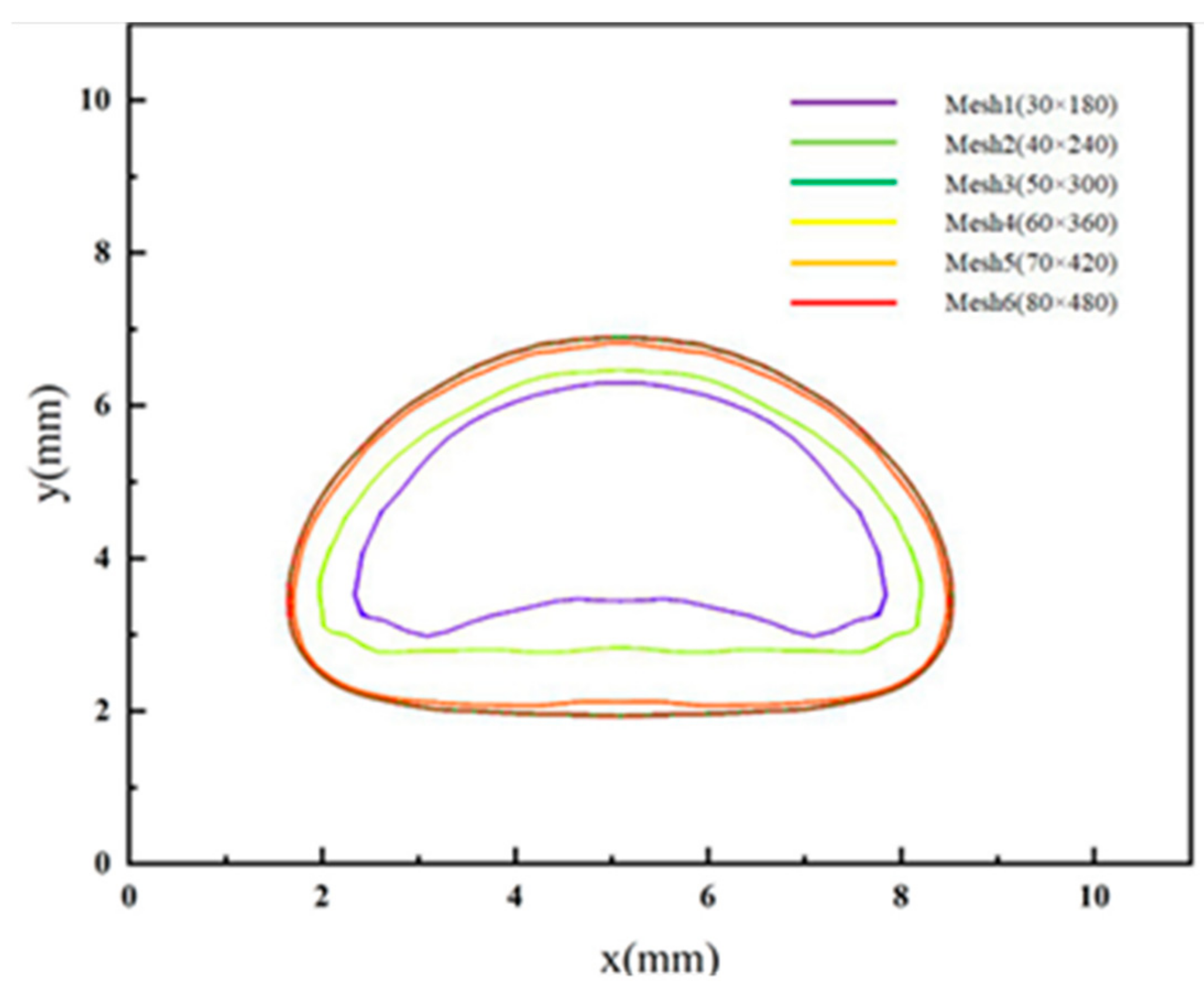
To ensure the reliability of CFD results, a grid independence study is conducted under six different grid sizes, which are Mesh1 (30 × 180), Mesh2 (40 × 240), Mesh3 (50 × 300), Mesh4 (60 × 360), Mesh5 (70 × 420), and Mesh6 (80 × 480). After initialization, bubbles contain 337, 629, 987, 1416, 1922, and 25,113 cells, respectively. Figure 5 shows the shape of bubbles at a certain moment in the process of condensation with different mesh sizes. It can be seen that, with the increase of mesh density, the shape of bubbles tends to be stable. The shape of bubbles has not change much after Mesh 3. Therefore, the Mesh 4 is selected to simulate the bubble condensation.

4. Results and Discussion

To validate the numerical model qualitatively and quantitatively, results from open literature [2] are used.

Table 2. Experimental conditions [6].

${\mathit{d}}_0 \left(\mathbf{mm}\right)$	$∆{\mathit{T}}_{\mathit{s}\mathit{u}\mathit{b}} \left(\mathbf{K}\right)$	${\mathit{P}}_{\mathit{p}} \left(\mathbf{kPa}\right)$	$\mathit{J}\mathit{a}$
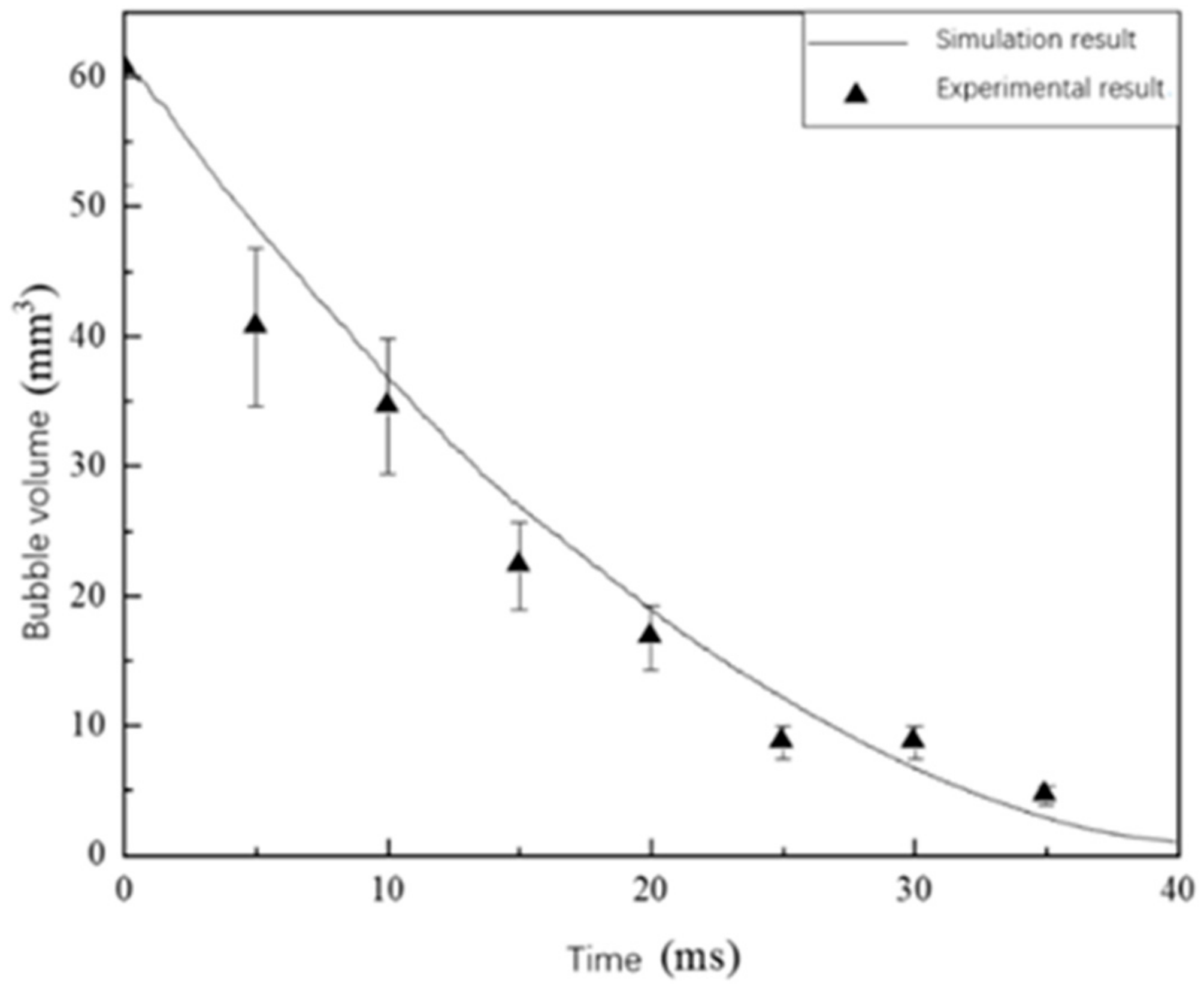
4.9	12	105	36

is the experimental condition, which is employed in the simulation, and the simulation result is compared with the experimental result, as shown in Figure 6. The error bar is ±15%. It can be seen that compared with experimental data, the simulated data are acceptable within a reasonable error range.

Figure 7a–c, respectively, shows the original high-speed cameral image, the bubble image after image processing, and the bubble volume contour of simulation results. The simulated bubble shows the same trend as the experimental result. By comparing the simulation results with the experimental results, the results obtained by using Formula (21) to process the phase change coefficient in the Lee model are reliable, laying a solid foundation for further study.

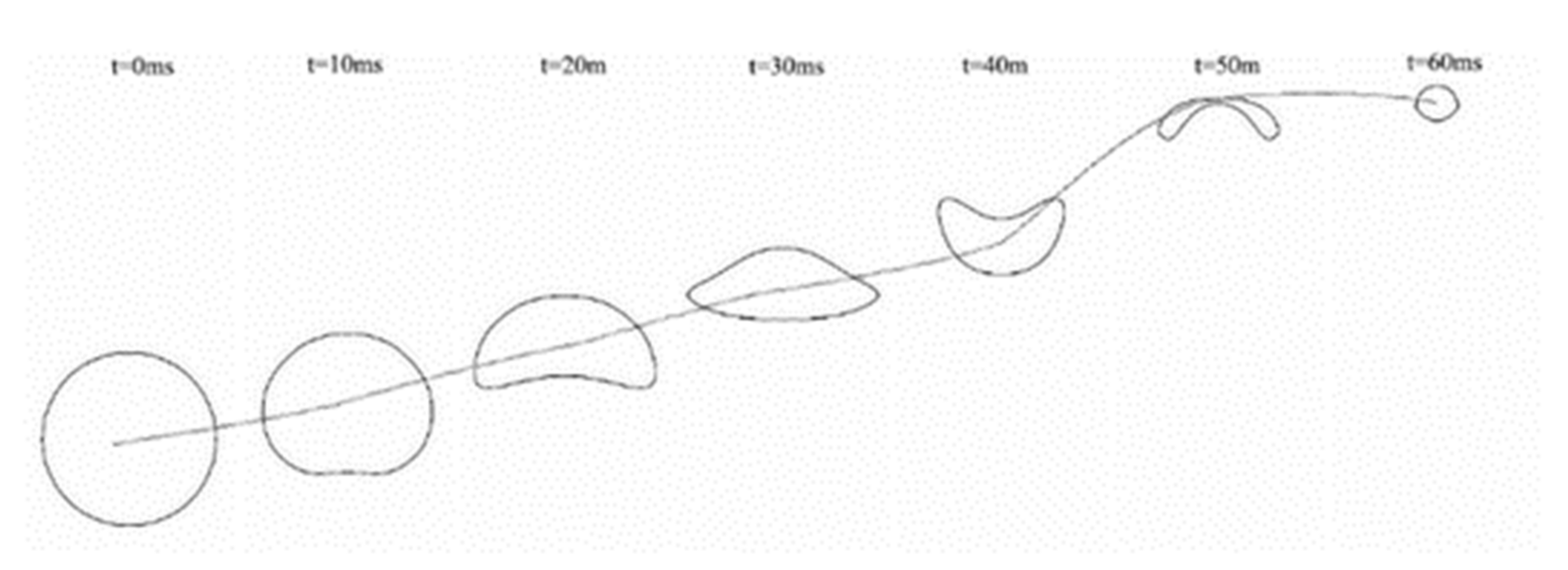
In order to analyze the bubble condensation process, numerical simulation is carried out, and the simulation conditions is shown in

Table 3. Simulation conditions.

${\mathit{d}}_0 \left(\mathbf{mm}\right)$	$∆{\mathit{T}}_{\mathit{s}\mathit{u}\mathit{b}} \left(\mathbf{K}\right)$	${\mathit{P}}_{\mathit{p}} \left(\mathbf{kPa}\right)$
6	10	101

, which is different from experimental conditions. Therefore, the bubble forms are very far from the camera images. As can be seen from Figure 8, as time goes on, due to the changes in the surrounding flow field and effect of surface tension, the bubble shape changes. The bubble shape gradually changes from a standard sphere to a flat sphere and a disk shape, and may even break in the middle. When the bubble shrinks to a certain size, the surface tension of the bubble takes the dominant role, and the bubble returns to spherical shape gradually. The bubble rises with time, reaching the maximum velocity between 40 ms and 50 ms, after which the velocity would decrease.

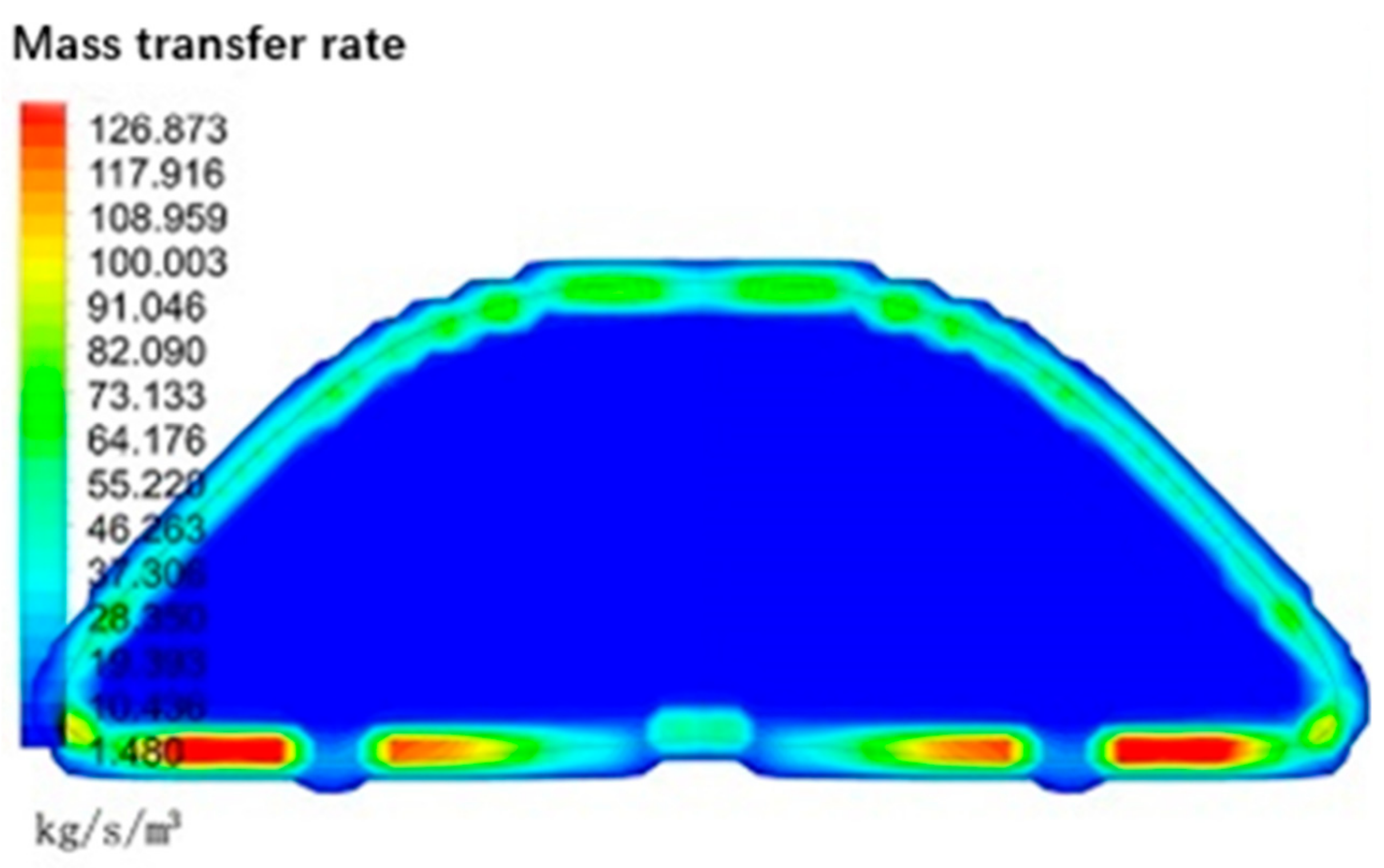
Figure 9 shows that the condensation phenomenon occurs at the gas–liquid interface in the process of bubble condensation, which is different from the method of calculating the total mass transfer by Nusselt number correlation formula and averaging the surface area of the bubble to obtain the mass source term. The mass transfer rate obtained by the Lee model is different. The mass transfer rate on the lower surface of the bubble is higher than the upper surface.

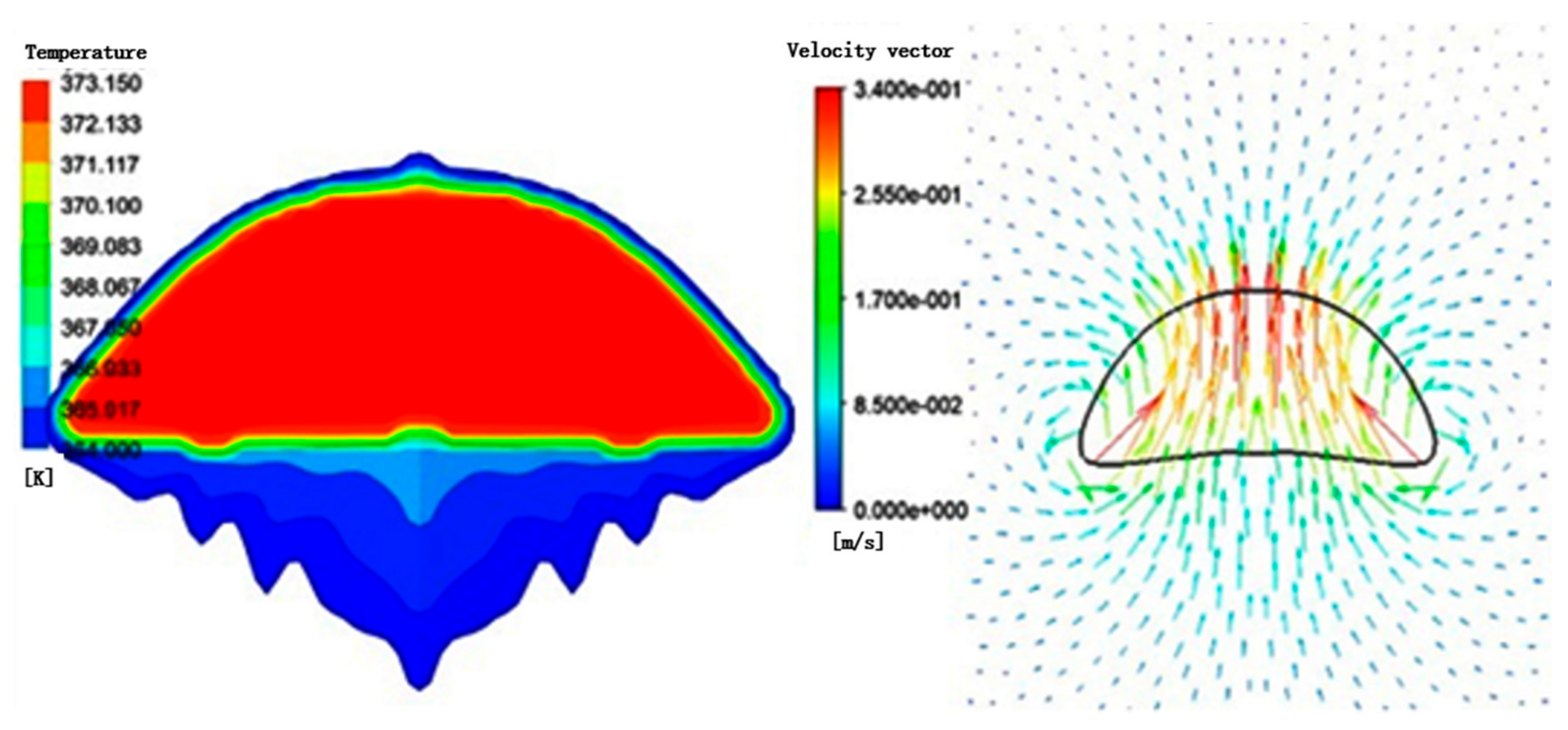
Temperature field cloud diagram and velocity vector diagram are shown in Figure 10. In the temperature field cloud map, the temperature at the center of the bubble remains saturated. Due to the effect of condensation, the liquid temperature at the bottom of the liquid slightly increases after the bubble wake. This region indicates that the condensation heat is given off from the interface and remarkable at the bottom of the bubble. The condensing bubble deformed by surface tension, drag force, buoyancy, inertial force of the surrounding liquid, and the condensation rate. When the bubble rising in the subcooled water, the bubble pushes the water out, causing the liquid to circulate, as shown in the velocity vector diagram. The heated water from all around the bubble interface flows down and accumulates at the bottom of the bubble, so the temperature of the water in this region gets higher. Due to the condensation rate is related to the water temperature, the different condensation rate induces small vortices at both sides end of the bubble. The presence of vortices alters the inertial force which in turn accelerates the bubble deformation and condensation rate.

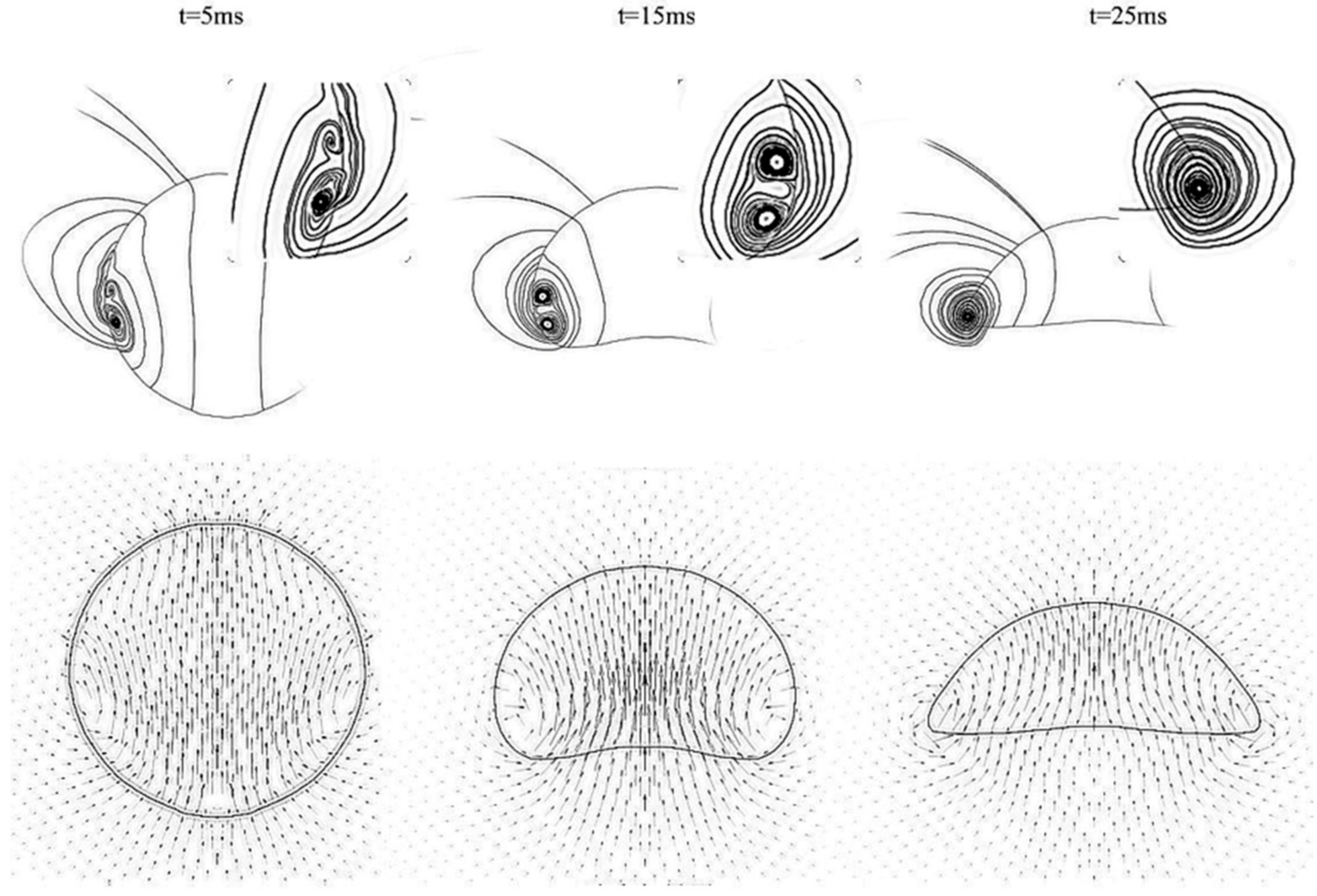
The flow diagram and velocity field of bubbles at different times in the process of rising and condensation are shown in Figure 11, which indicates that the bubble becomes flat spheres and one or two vortices are generated at the left and right ends of the bubble. Although vortices are various in shape, they all reinforce the heat transfer. As vortices disturbed the flow field and facilitates the exchange of hot and cold water around the bubble. The vortex magnitude is proportion to the density of the velocity vector. In addition, the velocity at the center of the bubble is relatively high and microcirculation of the vapor inside the bubble is generated.

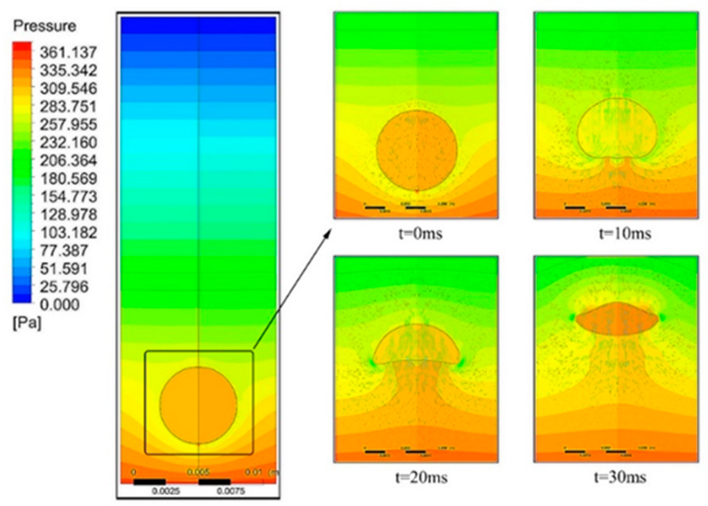
Due to the influence of gravity, the pressure increases gradually with the decrease of the height in water, but in order to maintain the shape of the bubble, according to the surface tension model theory, the pressure inside the bubble is higher than that around it, as shown in Figure 12. At different moments, the pressure field changes with the change of velocity field due to the difference of surrounding flow field.

5. Conclusions

Numerical simulation is performed to predict the process of bubble condensation. PID algorithm is adopted to correct the phase change coefficient of the Lee model, and the correlation formula of the phase change coefficient of the Lee model meeting the requirements is obtained. Summary of the results are itemized below.

(1)

Although the Lee model is widely used to simulate phase change, CFD simulation results ate highly sensitive to the value of phase change coefficient, which needs to be adjusted for different working conditions. In this paper, the phase change coefficient is corrected in various working conditions, and Formula (21) is obtained to adjust the value of phase change coefficient in different working conditions. Compared with experimental correlation (19), the feasibility of using the phase change coefficient adjustment formula to simulate bubble condensation is verified;

(2)

In the process of bubble rising, disturbance is generated with the fluid. The steam inside the bubble creates microcirculation, and several tiny vortices are generated on the side of the bubble, which accelerates the heat and mass transfer rate at the gas–liquid interface;

(3)

When the bubble condenses in subcooled water, the mass transfer rate at the interface varies from place to place and the pressure inside the bubble is higher than that around it.