Abstract
The amount of oil that is contained in the Canadian oil sands represent the third largest oil accumulation in the world. Approximately half of the daily oil production from the oil sands comes from mining processes and the other half is produced mostly using steam assisted gravity drainage (SAGD). This method is effective at reducing the viscosity of the oil. However, the generation of steam requires a significant amount of energy. Thus, there is an ongoing effort to reduce the energy needed to produce oil from the oil sands. In this article the intermittent injection of a solvent, along with steam, is investigated as a means of reducing the amount of energy required to extract oil from the Canadian oil sands. A simulation-based study examined the effect of the type of solvent, the cycles’ duration, the solvent concentration and the number of cycles. The simulations covered a time span of 10 years during which several different solvents (methane, ethane, propane, butane, pentane, hexane, and CO2) were injected under varying injection schedules. The solvents that were investigated are compounds that are likely to be readily available at a heavy oil production site. The solvent injection periods ranged from six to 24 months in length. The results reveal that SAGD combined with intermittent injection of hexane resulted in the most significant improvement to the cumulative oil production and in the cumulative energy-oil ratio (cEOR). Compared to SAGD without solvent injection, the cumulative oil production was increased by 45% and the cEOR was reduced by 23%. It was also seen that the performance of the proposed process is highly dependent on the resulting physical properties of the solvent-bitumen mixture. Finally, a simplified economic analysis also identified SAGD with intermittent hexane injection as the scheme that resulted in the highest net present value. Compared to SAGD without solvent injection, the intermittent injection of hexane led to an 85% increase in the net present value.
1. Introduction
Most of the daily activities performed by people around the world are highly dependent on a stable and lasting source of energy. Amongst the various sources of primary energy, oil accounts for the largest share [1]. According to the BP Statistical Review of World Energy, the proved oil reserves in the world are nearly 1.6 trillion barrels [2], which is expected to last for at least 50 years. However, increasing amounts of this oil is expected to come from unconventional sources, which are considerably more difficult and expensive to extract.
Canada’s oil sands are a perfect example of such an unconventional source. The oil that is contained in these reservoirs is commonly called bitumen and its principal characteristic is its inability to flow at original conditions due to its high viscosity and density. Currently there are two commercial pathways for extracting bitumen from the oil sands: Mining and in situ recovery. Mining works for shallow deposits (up to 75 m below the surface) and the amount of oil that can be recovered through this process is about 20% of the total original oil in place (OOIP). The remaining oil is extracted through in situ processes. Presently, the only processes that are being used to extract the oil in situ are related to thermal methods.
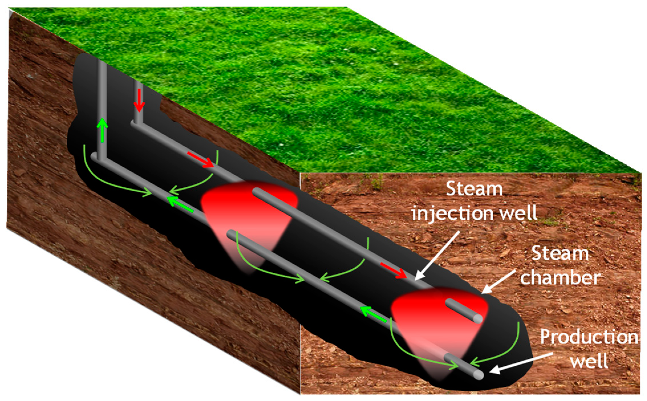
Thermal recovery methods are enhanced oil recovery (EOR) techniques based on the reduction of the viscosity due to heat transfer. This heat transfer can come from the injection of a hot fluid, such as steam [3] or it can be produced internally (in situ combustion [4] or electric heating [5]). Steam assisted gravity drainage (SAGD) [3] is the most used thermal recovery method and it consists of injecting steam into the reservoir in such a way that it develops a hot zone that heats the oil until its viscosity is low enough so that it flows under the effect of gravity (Figure 1). SAGD operations require two horizontal wells: The upper well is a steam injection well and the lower well is a producer well. This well receives the oil which flows naturally once its viscosity had been reduced.

Figure 1.
Steam assisted gravity drainage. A horizontal well injects steam into the reservoir and the heat transfer from the steam to the rock and fluids reduces the viscosity of the oil, which flows by the effect of gravity towards a producer well at the bottom of the reservoir.
Numerous improvements to the original SAGD process [3] have been proposed in order to make thermal recovery processes more efficient in terms of its energy requirement and profitability. Some examples of these variations include non-condensable gas-SAGD (NCS-SAGD) [6], single well-SAGD [7], X-SAGD [8] and expanding-solvent steam assisted gravity drainage (ES-SAGD) [9]. Of these improvements, the ES-SAGD process, in which solvent is injected with the steam, has shown promise. The main purpose of this variation is to reduce the oil viscosity while further reducing the amount of steam that is being used. The two most critical aspects of this method are the amount of solvent that is added to the steam and the amount of solvent that is recovered at the end of the process. This is particularly important because the solvents that are normally used may be more expensive than both the injected steam and the produced oil. In the remaining subsections of this introduction section, a more detailed overview of SAGD and ES-SAGD research will be presented.
1.1. Steam Assisted Gravity Drainage (SAGD)
SAGD was originally proposed by Butler [3] as an alternative to conventional steamflooding, in which the oil is pushed by injected steam towards a producing well. SAGD, on the other hand, uses gravity as the main driving force for oil movement. Butler reasoned that if steam were injected above a horizontal production well, the steam would move to the top of the reservoir and the warmed oil would eventually move downwards towards the production well. Additionally, steam injection causes the steam chamber to start expanding gradually until its size covers a considerable volume of the reservoir in which the oil would eventually start to move towards the production well [3].
Figure 2 illustrates the cross-section of a typical SAGD scheme. Steam is injected horizontally near the bottom of the reservoir, from where it rises upwards while the heated oil and condensate flow downwards towards a horizontal production well, which is approximately 5 m below the injection well. Generally, the steam injection pressure is kept constant during the whole process and the drawdown pressure at the producer is very small. This configuration ensures that the whole mechanism relies almost completely in gravity and not on a pressure difference, which is the case in many other types of fluid injection.
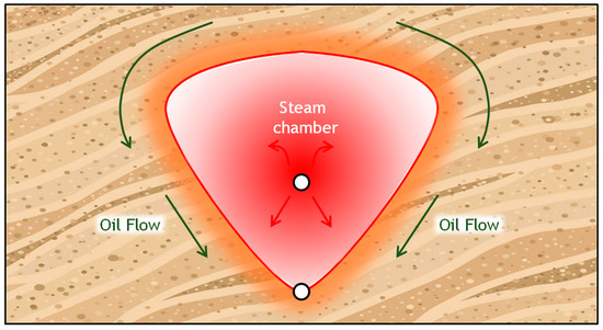
Figure 2.
Two-dimensional view of the steam chamber in a steam assisted gravity drainage (SAGD) process. The steam chamber is saturated with the injected steam. The oil flows at the interface of the chamber where the temperature corresponds to the saturation temperature at the injection pressure.
1.2. Expanding Solvent Steam Assisted Gravity Drainage (ES-SAGD)
The reduction in viscosity in SAGD can be further enhanced if, in addition to the heat transfer from the steam, there is also a mass transfer of solvent into the oil. ES-SAGD combines these two effects to improve recovery performance. Figure 3 shows that in ES-SAGD the oil drainage occurs in two different layers: A solvent boundary layer, where the oil viscosity is reduced due to the combined effect of dilution from the solvent and heat transfer from the steam, and a thermal boundary layer where the presence of solvent is negligible and the oil viscosity reduction is caused only by the heat transfer from the steam. Thus, the oil viscosity reduction in an ES-SAGD process is the result of the combined effect of the heat transfer from the steam and mass transfer from the solvent.
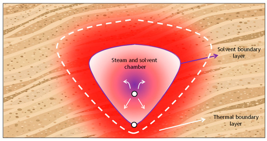
Figure 3.
In an expanding-solvent steam assisted gravity drainage (ES-SAGD) process two boundary layers are identified: A solvent boundary layer, that is formed by the combined effect of the steam and solvent injected, and a thermal boundary layer that separates the region of the reservoir that is affected by the heat transfer and the region that is still at the initial temperature.
The ES-SAGD process was first presented by Nasr et al. [9] as a “novel approach for combining the benefits of steam and solvents in the recovery of heavy oil and bitumen”. The process was tested in laboratory experiments in which the co-injection of steam with condensable hydrocarbon solvents (propane and octane) was compared with the injection of pure steam. The results from the ES-SAGD laboratory tests showed an improved oil recovery and reduced steam consumption. In other words, the heat transfer from the steam plus the mass transfer from the solvent reduces the oil’s viscosity but, with less steam than SAGD. It should be noted, however, the cost of the solvent can significantly affect the profitability of the process if a significant amount of solvent is left in the reservoir at the end of the process. Regarding the environmental consequences of the solvent injection, a recent study from the Alberta Energy Regulator (AER) classified the risks associated with this injection as low or middle according to 20 possible scenarios that could result in the release of contaminates of potential concern in a solvent-steam process [10].
Gates and Chakrabarty [11] used a genetic algorithm coupled with a numerical simulator to optimize the best injection strategy in an ES-SAGD process in terms of the cumulative net energy to oil ratio. The injection pressure and the solvent concentration in the steam were modified in multiple runs in order to know which was the combination that generates the lowest energy-to-oil ratio. The changes that were performed in these two variables led to a wide range of results, which provided evidence of the importance of the injection strategy in the performance of the process. One of the conclusions of this work was that the steam and solvent injected should not be in excess, but just enough to supply heat and solvent to the bitumen layer at the edges of the steam chamber.
1.3. Cyclic Expanding Solvent Steam Assisted Gravity Drainage
In cyclic ES-SAGD, the solvent is injected with the steam intermittently instead of continuously. Similar to ES-SAGD, the oil viscosity reduction in cyclic ES-SAGD is caused by both heat and mass transfer. However, unlike ES-SAGD, the temperature and solvent concentration at the steam chamber interface will change depending on whether steam or steam plus solvent is being injected.
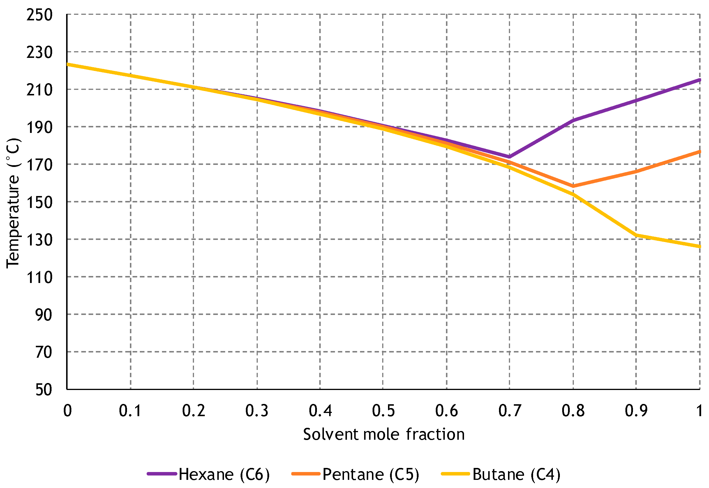
In SAGD, the temperature at the interface corresponds to the saturation temperature at the injection pressure. However, in ES-SAGD, the presence of the solvent in the steam chamber modifies the temperature and concentration at the interface because of a reduction in the steam partial pressure in the mixture. This, in turn, will lead to a lower temperature at the interface. This means that for ES-SAGD, the interface temperature corresponds to the two-phase vapour–liquid equilibrium temperature for solvent and steam at the injection pressure. This temperature is always lower than the pure steam saturated temperature at the same pressure. Figure 4 shows the variation of saturation temperature for different steam-solvent mixtures in the vapor phase according to solvent concentration.
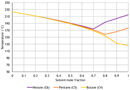
Figure 4.
Saturation temperatures depending on solvent concentration for various mixtures of steam and solvent at 2500 kPa (generated by using WinProp (CMG, Computer Modeling Group) [14]).
A previous study in which a similar process to cyclic ES-SAGD was tested, was conducted by Zhao [12] in 2007. He proposed a new recovery process called steam alternating solvent (SAS). This process was a combination of SAGD with vapor extraction (VAPEX) in which solvents in vapor form are injected instead of steam [13]. SAS consists of alternating the injection of steam and solvent. The main difference with cyclic ES-SAGD is that in SAS the solvent cycle consists of pure solvent in vapor phase instead of steam-solvent co-injection. The process starts in the same way as SAGD until the heat losses to the overburden becomes significant. At that moment, the injected fluid is changed to solvent until the chamber temperature is reduced. This cycle is repeated until it is no longer economical to continue. Zhao used numerical simulations to analyze the process and concluded that the production rate that is achieved with SAS could be as high as that of a SAGD process while the energy input per unit of oil recovered is 18% less than SAGD. Furthermore, Zhao explained that the performance of SAS depends on the duration of steam and solvent injection periods.
Although in most cases a numerical reservoir simulator is used as the main tool to analyze and understand a process such as ES-SAGD, it is important to include the information that comes from laboratory experiments and combine this information with the results that are obtained in a reservoir simulator. Zhang et al. [15] analyzed the huff-and-puff injection of CO2 in tight reservoirs considering the molecular diffusion and adsorption. In their study, Zhang et al. matched a reservoir simulation model against experimental core tests to demonstrate the importance of diffusion and adsorption in the CO2 storage for tight formations. Similarly, Janiga et al. [16] optimized the operational conditions of a huff-and-puff process using a data-driven model that was built using advanced laboratory experiments.
1.4. Aim of the Study
The aim of this study is to numerically simulate and analyze the application of ES-SAGD in a cyclic manner. The simulations will test various pure solvents and, in a given simulation, the duration of solvent injection cycles may be variable. Additionally, the simulation may begin with either pure steam injection or with steam plus solvent injection. The best-case scenario will be the combination of solvent and solvent injection cycles which allow ES-SAGD to increase oil production (relative to SAGD) while simultaneously minimizing solvent usage. A subsequent economic analysis will be undertaken in order to provide additional insight on which is the best choice of operating parameters.
2. Reservoir Simulation
2.1. Description
Reservoir simulation provides a quantitative means to predict the performance of a recovery process for a given set of well configurations operating conditions. Numerical thermal reservoir simulators are particularly useful in modeling recovery processes in which the change in reservoir temperature affects the fluid properties. Most current SAGD projects rely on numerical simulations to analyze reservoir behavior and to forecast future performance [17,18]. This section contains a brief summary of the equations that are solved in a commercially available reservoir simulator. The following equations are presented for the benefit of interested readers however, those who are already familiar with the subject can go immediately to the following section with no loss of continuity.
At each time step, the simulator solves the mass, energy, and momentum conservation equations. The overall conservation of mass in a porous media is expressed as:
where the left-hand term represents the accumulation, which is calculated considering the reservoir porosity () and the fluid density (), and the right-hand term contains the flux and the injection/production (). The flux is calculated considering the velocity () of the fluid in the reservoir. Subsequently, the component mass conservation equation can be written as follows:
In this equation, and represent the molar fraction and molar density of component i in a particular phase, while is the saturation of that phase in the cell. The subscripts , and indicate the phases water, oil, and gas respectively while the subscript is referred to the component that is being solved. Generally, one component is used to model the water and two components are used to model the oil. In some cases, they are called “pseudo-components” because they come from a lumping process which included multiple components. These pseudo-components represent a heavy and light fraction of the bitumen, which is generally composed solely of methane.
The conservation of energy can be expressed with the following equation:
Equation (3) takes into account that the mass of each component is stored only in the pores of the rock while heat is stored not only in the pores but in the rock matrix. Generally, three phases are assumed to be present in the simulations: Oil, gas, and water. and represent the heat capacity of phase and the solid (rock) at a fixed volume while is the heat capacity at fixed pressure. Additionally, is the density of the solid and is the bulk thermal conductivity, which takes into account the fluid and rock thermal conductivity. The thermal conductivity is generally expressed as a tensor, however in this study, because the reservoir is considered isotropic, the thermal conductivity is a scalar. Finally, and represent the heat source or sink and the heat lost to the overburden or understrata, respectively.
In Equations (2) and (3), the velocity of each phase is calculated using Darcy’s law:
where is the viscosity of phase , is the relative permeability of phase , K is the absolute permeability of the reservoir rock, is the pressure of phase , is the density of phase , z is the elevation, and g the acceleration of the gravity force.
In order to solve the equations previously described, the boundary and initial conditions were defined. At the external side boundaries as well as the top and bottom boundaries of the domain, no flow and no heat transfer boundary conditions were applied:
The initial condition can be defined as:
where represents the spatial domain.
The initial condition is the original temperature at the overburden:
The temperature boundary conditions at the top and bottom of the reservoir are:
Along with the previous equations, the effect of diffusion on the flux of component i () in each phase is calculated through:
where represents the tortuosity of phase in a particular direction and is the molecular diffusion coefficient of component i in phase .
All of the simulations were performed by using the STARSTM reservoir simulator [19] which solves Equations (1)–(4) subject to Equations (5)–(9) by using the finite volume method. The equations are discretized (by dividing the domain into discrete grid blocks) yielding a set of non-linear partial differential equations which are subsequently linearized and solved by using Newton’s method at each time step using an implicit time integrator [19]. There are two ways of initializing a reservoir simulation model. The most common is defining a pressure at a datum level depth. The pressure at other locations is calculated knowing the fluids’ densities and the depth of each of the zone’s contacts. This is generally known as initialization by equilibrium. An alternative methodology is defining the pressure at each of the cells which is called initialization by enumeration. In this study, the reservoir simulation model was initialized using a constant saturation and pressure according to what is explained in the next section.
2.2. Reservoir Model
Table 1 shows the main reservoir properties that were used in the current study. The reservoir was assumed to be homogeneous with no aquifers or any gas cap in the model. The values listed in Table 1 were taken from previous numerical studies in the Canadian Athabasca region: The permeabilities, porosity, and initial oil saturation were taken from Shin and Polikar [20], the initial reservoir pressure and the thermal properties are the ones used by Rabiei [21], the diffusion coefficients for each solvent correspond to the ones obtained by Salama and Kantzas [22] while the endpoints for the relative permeability curves were taken from Gates [23]. The effect that the presence of solvent has in the relative permeability curves and hence in the fluid displacement in the reservoir, was not taken into account in this study. This change in the relative permeability curves can alter the shape and growth of the steam chamber and, consequently, the performance of the process. This effect will be considered in future studies.

Table 1.
Reservoir properties used in the simulation model.
Due to the symmetry and homogeneity of the reservoir, a two-dimensional (2D) reservoir was used to represent the original three-dimensional (3D) reservoir. Representing the 3D reservoir with a 2D reservoir significantly decreases the total computational time. The authors realize that this assumption neglects the pressure drop in the horizontal section of the well and it also implies that the steam chamber will grow in the same way and at the same speed throughout the whole length of the well. However, the current study is intended to serve as a first step in investigating the feasibility of cyclic ES-SAGD processes and thus, a rigorous 3D simulation will be a follow-up to the current study.
The resulting reservoir model is 50 m wide and 30 m high and, taking into account that the wells are located at the middle of the cell, the distance between the producer and injector is 5 m and the distance from the producer to the bottom of the reservoir is 1.5 m. Regarding model cell size, it was considered that cells of 1 m (cross-well) × 1 m (vertical) were appropriate for the simulation. Nevertheless, an additional 2D model with a cell size of 0.5 m (cross-well) × 0.5 m (vertical) was also tested in order to compare oil production rate and volume. This comparison did not show considerable differences regarding oil rate and cumulative oil production for both SAGD and ES-SAGD cases. Thus, the 1 m × 1 m grid was considered adequate for the current study. Figure 5 shows the distribution of the grid cells as wells as the location of the wells with respect to the grid.
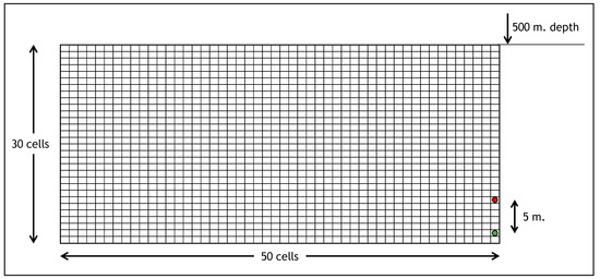
Figure 5.
Location of the wells and cell sizes in the two-dimensional (2D) simulation model.
The reservoir oil was modeled as a live-oil using two pseudo-components: One light pseudo-component that was composed of methane and had a concentration of 4 mol% in the mixture and a heavy pseudo-component which represents bitumen. In the plots that are shown in the next sections, the cumulative oil production refers to bitumen. The oil had a molecular weight of 590 g/mol, density of 1012 kg/m3 and saturation pressure of 3200 kPa. These are typical values for oil from the Athabasca oil sands deposit according to Strausz and Lown [24]. These characteristics and composition were the matching-parameters used to define the a,b coefficients and the binary interaction coefficients of the Peng-Robinson Equation of State. Table 2 contains the fluid properties that were used in the simulator. These values are in agreement with the experimental values reported by Strausz and Lown [24].
Table 2.
Fluid properties for the oil used in the simulation model.
All simulations included two wells. The injection well had a constraint of maximum bottom hole pressure of 2500 kPa while the production well had a constraint of a maximum steam rate of 1 m3/day. The quality of the injected steam was set to 0.8. This quality was also used by Rabiei [21] and Gates [23] who conducted similar simulation studies. Neither of these constraints nor the well locations were changed in any of the simulation runs. The parameters that were varied were related to the solvent type and the duration and schedule for solvent injection. The total length of all simulations was 10 years and for all the simulations, a period of four months at the beginning of the simulation was established as the pre-heating stage.
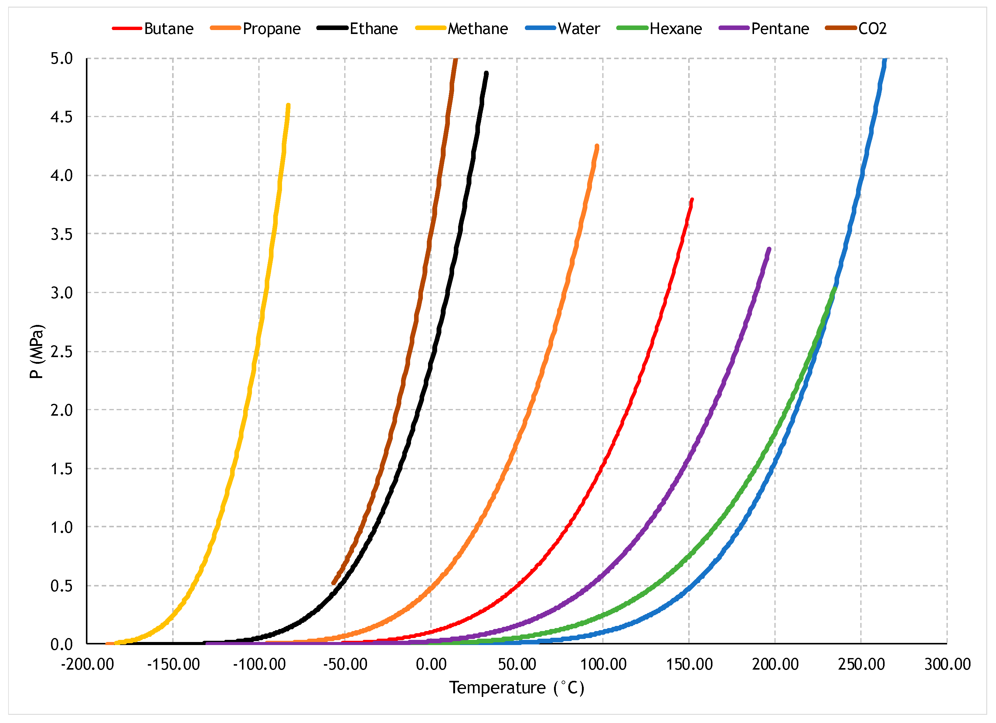
The solvents that were co-injected with the steam in the simulations represent pure component solvents whose physical properties were taken from the internal library of the simulator. Figure 6 shows a vapour–liquid equilibrium diagram for all solvents and water.
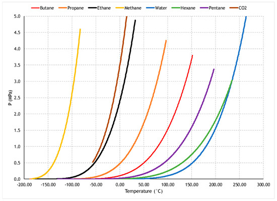
Figure 6.
Vapour–liquid equilibrium diagrams for the solvents that were co-injected with the steam in the simulations.
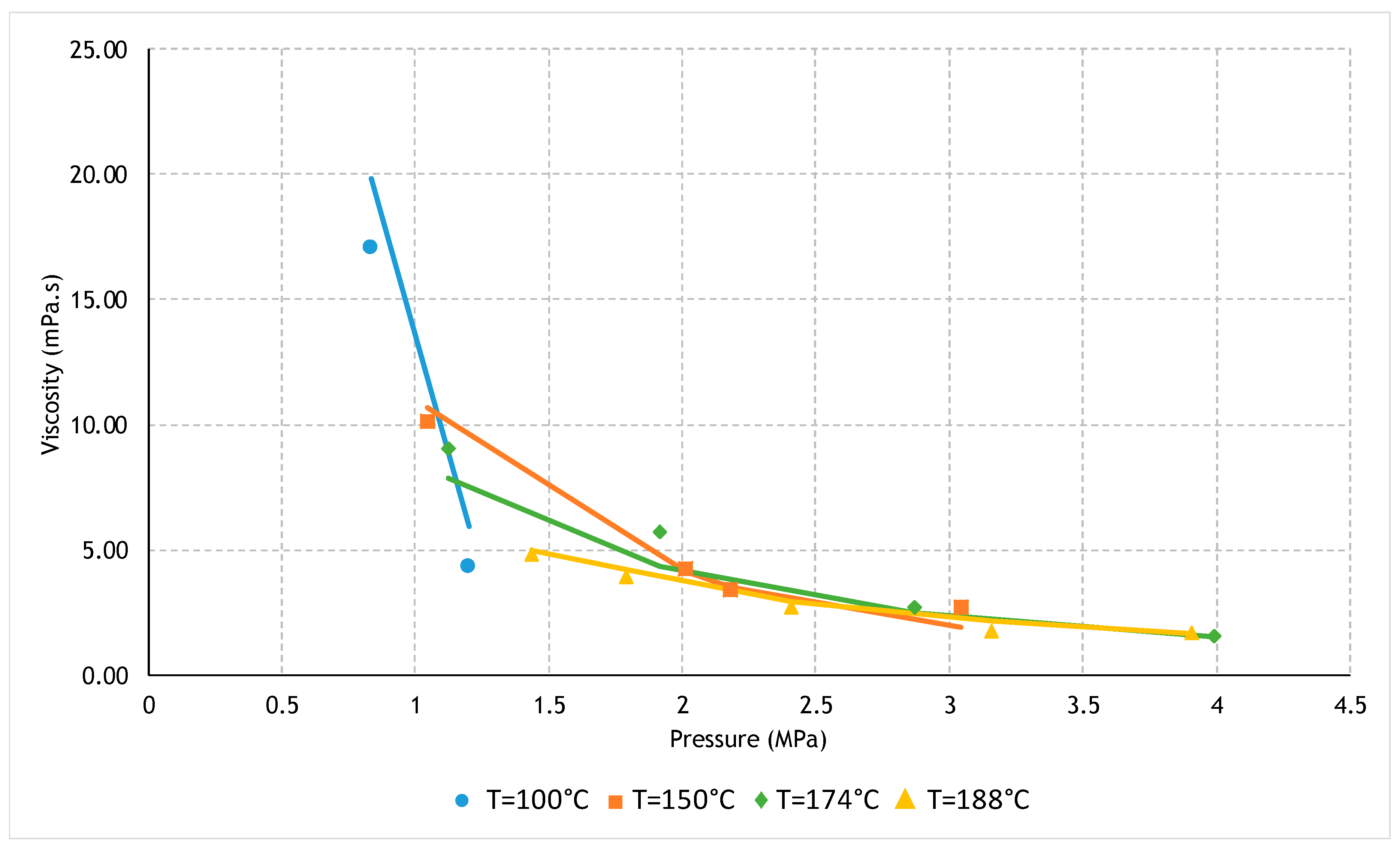
The bitumen-solvent viscosity was modeled using a correlation developed by Pedersen et al. [25], which is included in the software WinProp (CMG) [14]. In this model, the viscosity of a mixture depends on the critical temperature and pressure of each component as well as their binary interaction coefficients. The results from this correlation were subsequently adjusted to the experimental values reported by Nourozieh et al. [26,27,28,29,30,31] and Haddadnia et al. [32] for each of the solvents. Figure 7 shows a comparison between the experimental and simulated values for the butane case. It can be observed that there is a good agreement between the values that were calculated through the correlation and the ones that were measured experimentally. The mixture viscosity calculated for the rest of the solvents showed a similar behavior when compared with the experimental data. This agrees with the observation by Nourozieh et al. [28] regarding the correlation from Pedersen et al. [25] and its ability to reproduce the viscosity behavior of different bitumen-solvent mixtures.
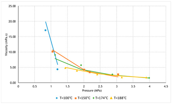
Figure 7.
Comparison between experimental and simulated viscosity values for mixtures of butane-bitumen at different equilibrium pressures and temperatures. The experimental values are represented by different symbols and were taken by Nourozieh et al. [28].
3. Results and Discussion
In this section, the results from numerical simulations of the SAGD and ES-SAGD process with different solvents and cycle durations and solvent mole fractions are presented. In the first set of cases, seven different solvents were injected continuously with the steam, at different concentrations. The results were analyzed in terms of the final cumulative oil production and energy efficiency. The second set of cases contains tests in which the cycle length is varied. These variations were made following a full factorial experimental design to identify which of these variables had the greatest impact on the cumulative oil production. The third and fourth sets of cases assess the impact that variations in the durations and scheduling of the steam-solvent cycles as well as the solvent mole fraction have in the performance of the process. This performance was analyzed taking into consideration not only the final oil production but also the amount of solvent retained in the reservoir at the end of the process. Finally, a preliminary economic analysis was conducted taking into account the fluids that were injected and produced as well as their costs.
3.1. Continuous Solvent Injection
Figure 8 shows the cumulative oil production for cases in which the solvents were injected continuously throughout the 10-years period, at various concentrations. The horizontal red line represents the cumulative oil production for a SAGD case. The cases in which carbon dioxide, methane, ethane, or propane were injected have a cumulative oil production that is considerably lower than the one obtained by injecting pure steam. These solvents are generally considered non-condensable gases. Their benefit in a SAGD process is not an increase of production but the reduction of the steam-oil ratio and heat losses to the overburden. Furthermore, it is important to take into account how, in the cases previously mentioned, the cumulative oil production is reduced according to the increments in the solvent concentration of carbon dioxide, methane, ethane, or propane.
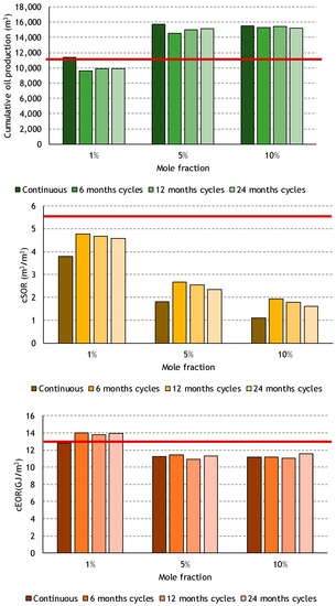
Figure 8.
Cumulative oil production, steam-to-oil ratio (cSOR), and energy-to-oil ratio (cEOR) for SAGD and ES-SAGD cases with different solvents and concentration. SAGD results are indicated with a horizontal red line.
In contrast with the non-condensable solvents, the cases in which butane, pentane, and hexane were injected show higher values for cumulative production than that of SAGD. These solvents not only can lead to a reduced steam usage but also to a further reduction of oil viscosity beyond that of heating alone.
The energetic performance of each solvent co-injection is also shown in Figure 8 in terms of the cumulative steam-to-oil ratio (cSOR) and cumulative injected energy-to-oil ratio (cEOR). The cSOR measures the amount of steam that is required to produce one unit of volume of oil whereas the cEOR is a measurement of the energy that is necessary to produce the same oil quantity. The cEOR takes into account the heating value of the solvent and the enthalpy of the steam. A lower value of cSOR does not necessarily mean that the amount of solvent that was injected in the reservoir is low but that this amount led to a higher increase of the cumulative oil production. For the co-injection of butane, pentane, and hexane, there is a significant reduction in the amount of steam usage in comparison with a SAGD process (horizontal red line). On the contrary, methane, ethane, propane, and carbon dioxide have higher cSOR than that of SAGD. For most of the solvents, the cSOR decreases with an increase in solvent concentration.
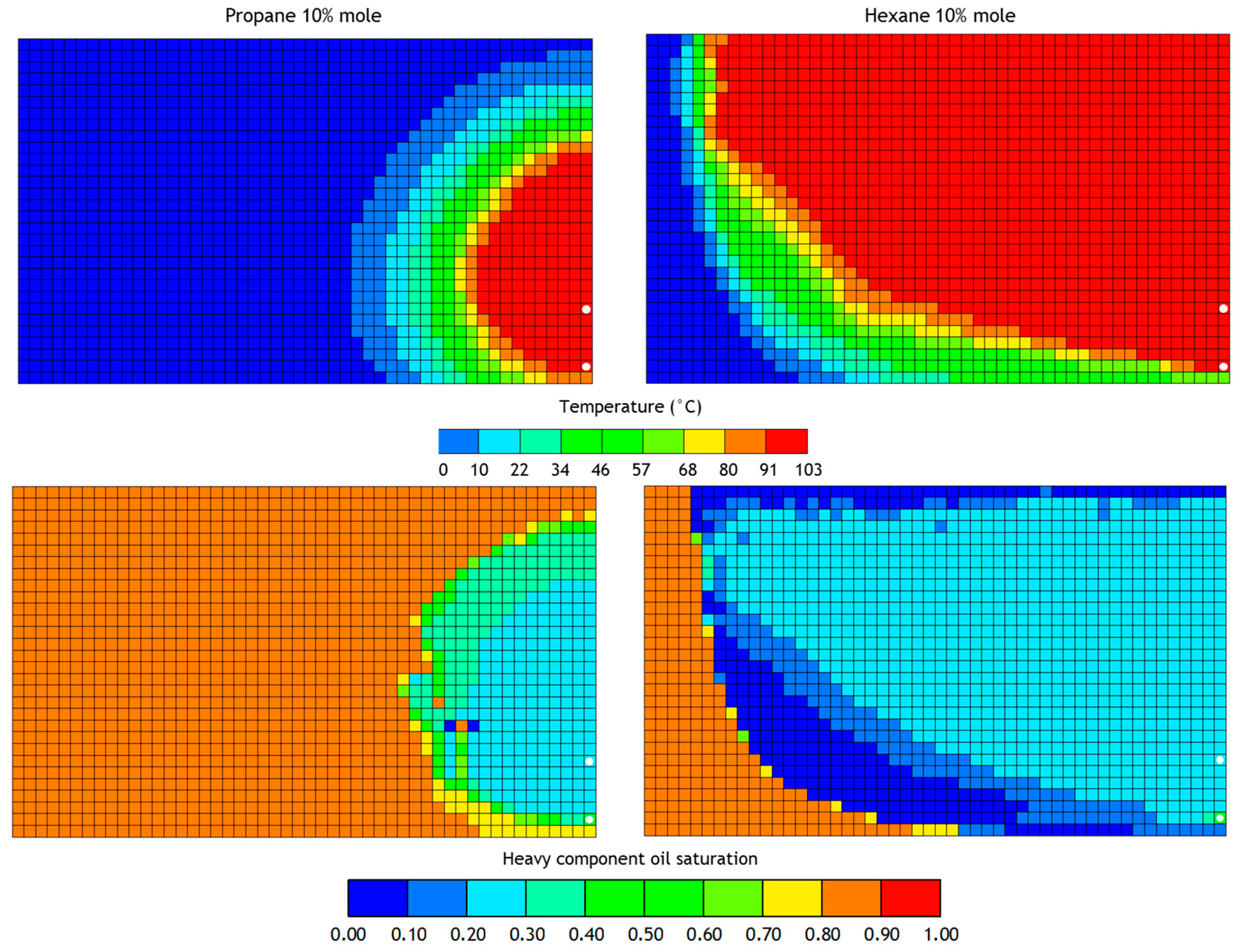
The effect of the solvent on the temperature distribution and fluids distribution inside the reservoir is shown in Figure 9. This plot shows how the temperature and the heavy component saturation in the oil phase vary spatially in the reservoir five years after the start of a continuous ES-SAGD process in which hexane (condensable) and propane (non-condensable) were injected at 10 mol%. The white circles at the bottom right corner represent the injector and producer wells. After five years, the propane co-injection case shows a steam chamber that has not reached the upper boundary of the model and, that has covered less than half of the area. On the contrary, the hexane steam chamber has spread over more than half of the area in the same time. This difference is likely an indicator of the relative rates of mass transfer of each of the two solvents into the bitumen.
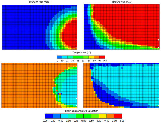
Figure 9.
Temperature and heavy component saturation in the oil phase distribution after five years of simulation for two ES-SAGD processes in which hexane and propane were co-injected at 10% mole. Hexane co-injection shows a bigger steam chamber after five years which leads to a higher oil recovery compared to the propane co-injection.
3.2. Impact of the Cycle Duration, Mole Fraction, and Start Mode in the Performance of the Cyclic ES-SAGD Process
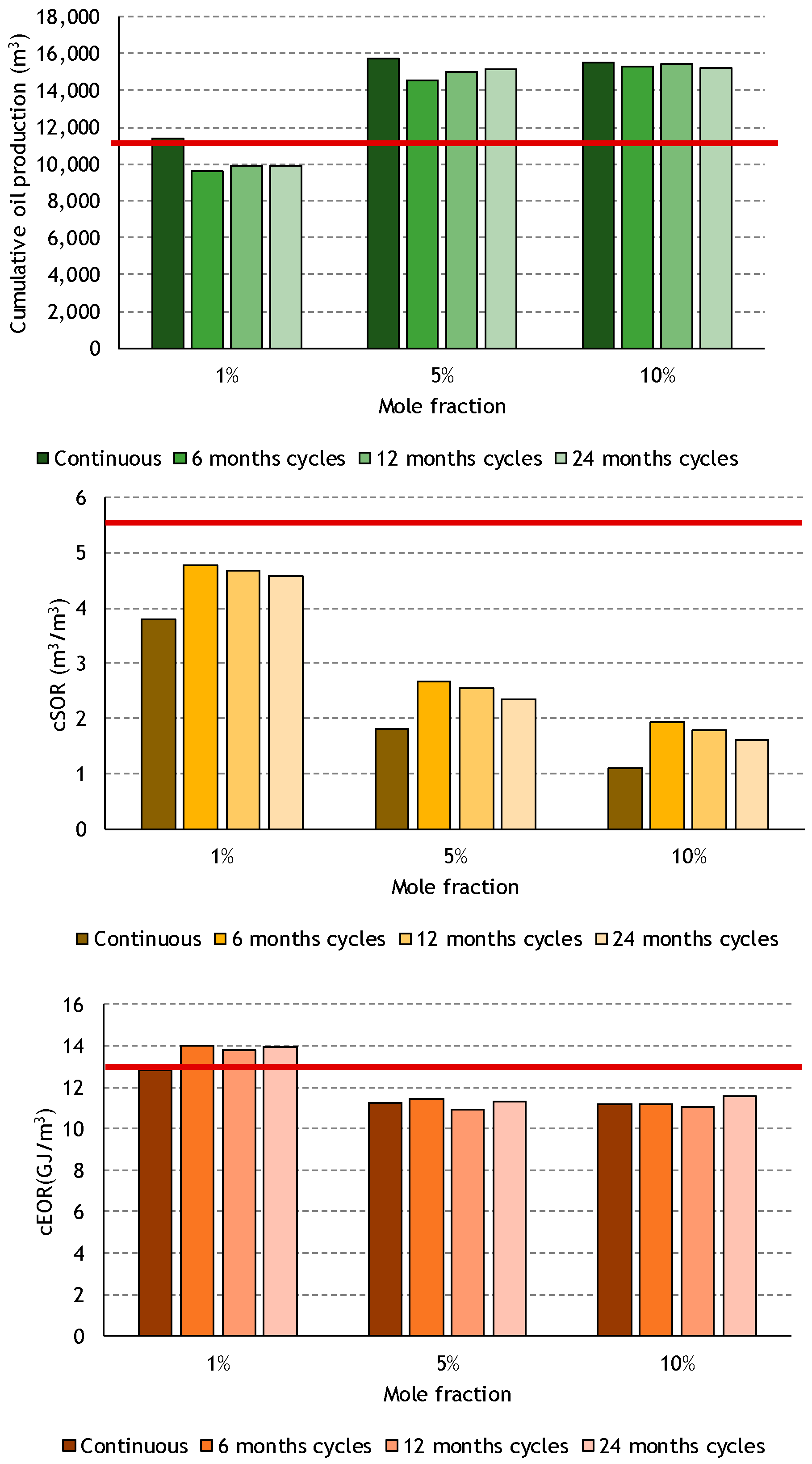
The objective of these cases was to determine how much impact cycle duration and solvent mole fraction had on the cumulative oil production for each of the solvent-steam mixtures. In the simulations, the mole fraction and the duration of the solvent co-injection cycle could take three possible values: The values for the solvent mole fraction were 0.01, 0.05, and 0.1 and for cycle duration were six, 12, and 24 months. The results from these simulations were used to assess the impact that each of the variables had on the final oil production. Figure 10 shows a Pareto plot that presents the impact of cycle duration and solvent mole fraction on oil production. In this plot, the average oil production for the cases in which the cycle duration or mole fraction had its highest value and the cases in which it had its lowest value was calculated. Subsequently, the difference between these results was divided by the average oil production of all the cases. In this way, the numbers on the horizontal axis represent the difference between the results that come from choosing a high or low value of cycle duration or mole fraction. These values were normalized with respect to the average oil production of all the cases. This calculation was performed for each solvent and for each start mode. The side in which the bars are placed in the plot whether the variable that is being analyzed has to increase or decrease to generate an increment in the cumulative oil production.
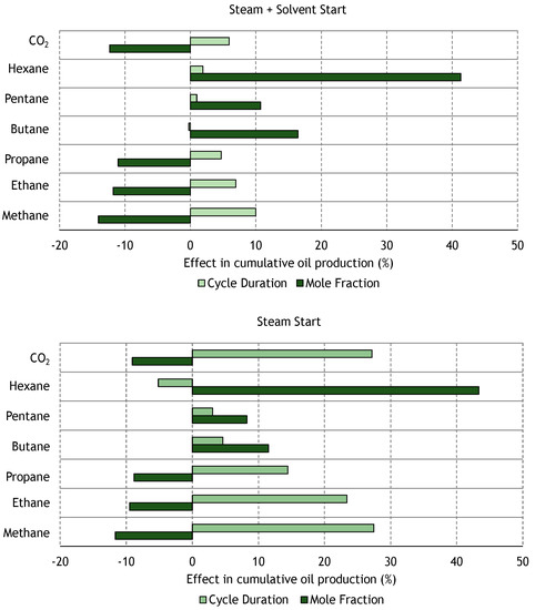
Figure 10.
Pareto plot that shows the impact of the cycle duration and mole fraction changes on the cumulative oil production for different solvents and different start modes.
As shown previously, regarding the continuous injection cases, there is a clear distinction between the behavior of the non-condensable solvents and the condensable solvents. For the non-condensable gases, increasing the solvent concentration always decreased the cumulative oil production. This agrees with the behavior observed in the continuous injection cases. For the condensable solvents (hexane, pentane, and butane), an increase in the solvent concentration led to an increase in the cumulative oil production. The above observations may be an indication that the relatively poor performance of the non-condensable solvents is due to their low solubility in bitumen. As seen previously in Figure 4, the differences between the performances of each of the solvents are related to the solvent solubility in the bitumen. The final reduction in the oil viscosity is directly dependent on the solvent content which, in turn, is defined by the type of solvent and its solubility as well as the temperature and pressure at which the process is taking place. As noted by Bahadori et al. [33] and by Zirrahi et al. [34], the solubility of the hydrocarbons in oil increases with carbon number where as the solubility of the hydrocarbons in water decreases with the carbon number. Carbon dioxide’s solubility in oil is comparable to that of ethane Zirrahi et al. [34]. However, the solubility of carbon dioxide in water is far greater than that of any of the hydrocarbon solvents Bahadori et al. [33]. Thus, the high solubility of carbon dioxide in water reduces its effectiveness as a solvent. The best operating strategy for an ES-SAGD process is defined by the conditions at which the oil phase viscosity is the lowest as it was described by Gates [23]. These conditions are not only related to the pressure and temperature of the process but to the solubility of the solvent that is being injected with the steam. Each solvent will have a different solubility in the bitumen at a particular pressure and temperature which will ultimately define the performance of each solvent in an ES-SAGD process regardless of the reservoir properties.
The results that were obtained in this section regarding the effect of cycle duration, are not conclusive. They suggest that an increase of cycle duration is beneficial for oil production regardless of solvent type or start mode. Nevertheless, for the case of hexane in which the initial cycle is pure steam, the highest oil production came from cases in which the duration of the solvent co-injection cycles was shorter. The relation between cycle durations and oil production is more complex than the one related to mole fraction. In the following sections, this relation will be explained through the results from additional simulations.
Finally, it is important to notice how there is a significant difference between the impact that the duration of the cycles has on the cumulative oil production depending on the start mode. The cycle duration has a higher effect for cases in which the first cycle corresponded to a pure steam cycle. This means that the order or timing of these cycles is also important because it will modify the way in which the steam chambers grows in the reservoir. This aspect will be better explained with additional simulations in a following section.
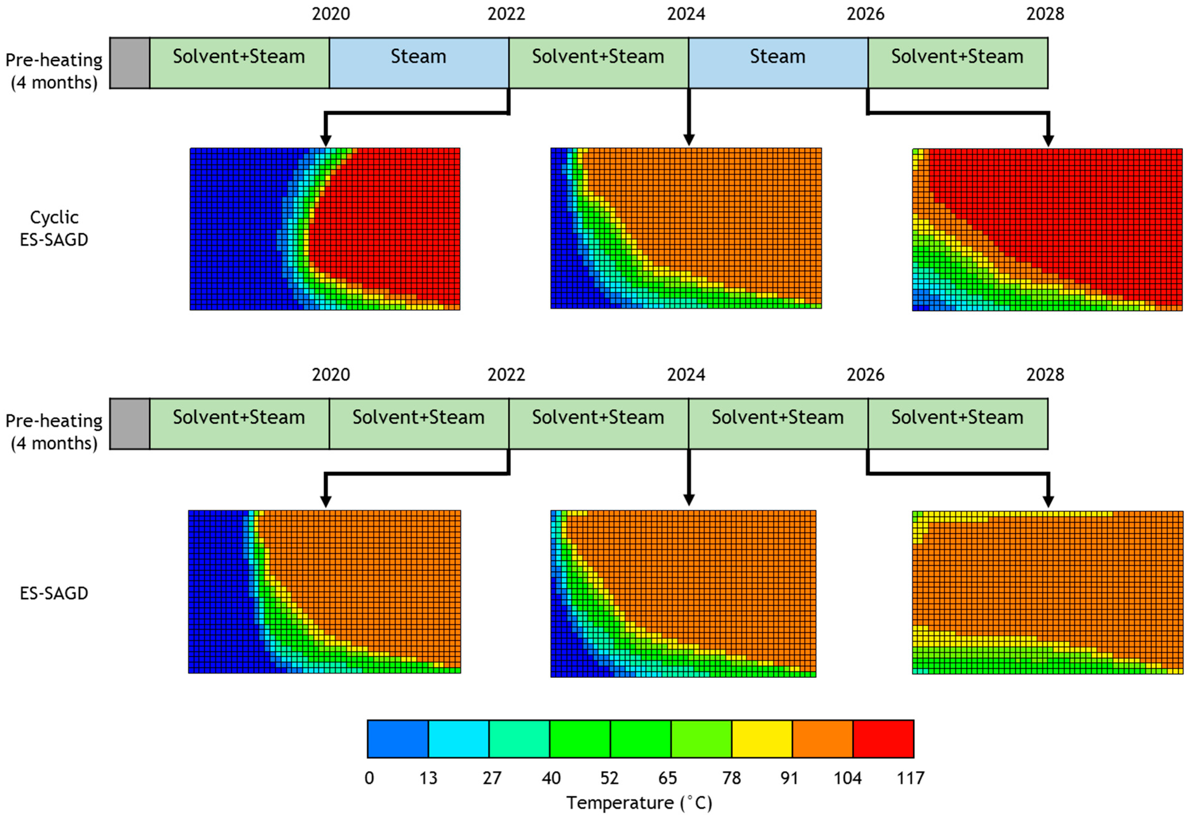
Figure 11 shows the temperature distribution for an ES-SAGD case with 10 mol% hexane and cyclic ES-SAGD with steam-solvent start in which the same solvent and concentration was used. The images are at the moment in which the change in the type of cycle occurs. In this case, cyclic ES-SAGD starts with a solvent co-injection and both processes behave identically until they reach year 2020 in which the pure steam injection cycle starts. At the end of this period, the temperature distribution as well as the steam chamber shape are considerably different in both processes. The temperature inside the steam chamber of cyclic ES-SAGD is higher because it represents the saturated temperature of pure steam instead of a steam-solvent mixture. If this temperature is higher, then the temperature gradient that goes from the chamber interface to the portion of the reservoir that is unaffected by the process is also altered. This temperature variation, and the fact that during the steam cycle the oil was not affected by the interaction with the solvent, leads to a different chamber. At year 2024, the chamber shapes are similar for both processes and at year 2026 they show important differences again due to the effect of the pure steam cycle. It is noted that at this moment ES-SAGD has already covered almost all the domain whereas in cyclic ES-SAGD there is still a small unaffected area. These plots show that the change of the temperature of the injected stream is altering the temperature inside the chamber and at the interface and this in turn affects oil mobility and drainage.
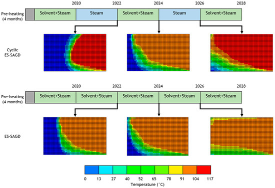
Figure 11.
Changes in the reservoir temperature and steam chamber shape at three different moments during the simulation of an ES-SAGD and SAGD process using hexane at 10% mole and two-years cycles.
3.3. Variations in the Duration and Timing of the Cycles
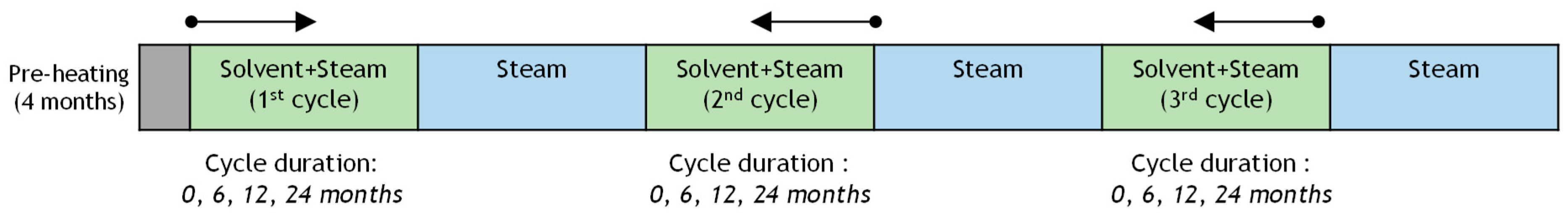
The main idea of this group of simulations was to determine the importance of the duration of each cycle and moment at which the solvent was co-injected. The solvent concentration was fixed at 10 mol% and the periods at which the solvent (hexane) was co-injected were changed between zero, six, 12, and 24 months, as illustrated in Figure 12. There were three intervals at which the solvent could be co-injected. After the duration of these intervals was defined, they were positioned evenly over the 116-month period of the total simulation (the first four months correspond to the pre-heating stage).
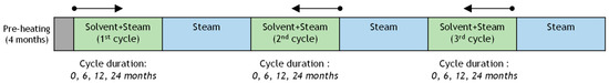
Figure 12.
Combinations of cycle durations for a group of simulations of cyclic ES-SAGD using hexane at 10% mole and three cycles of solvent-steam injection.
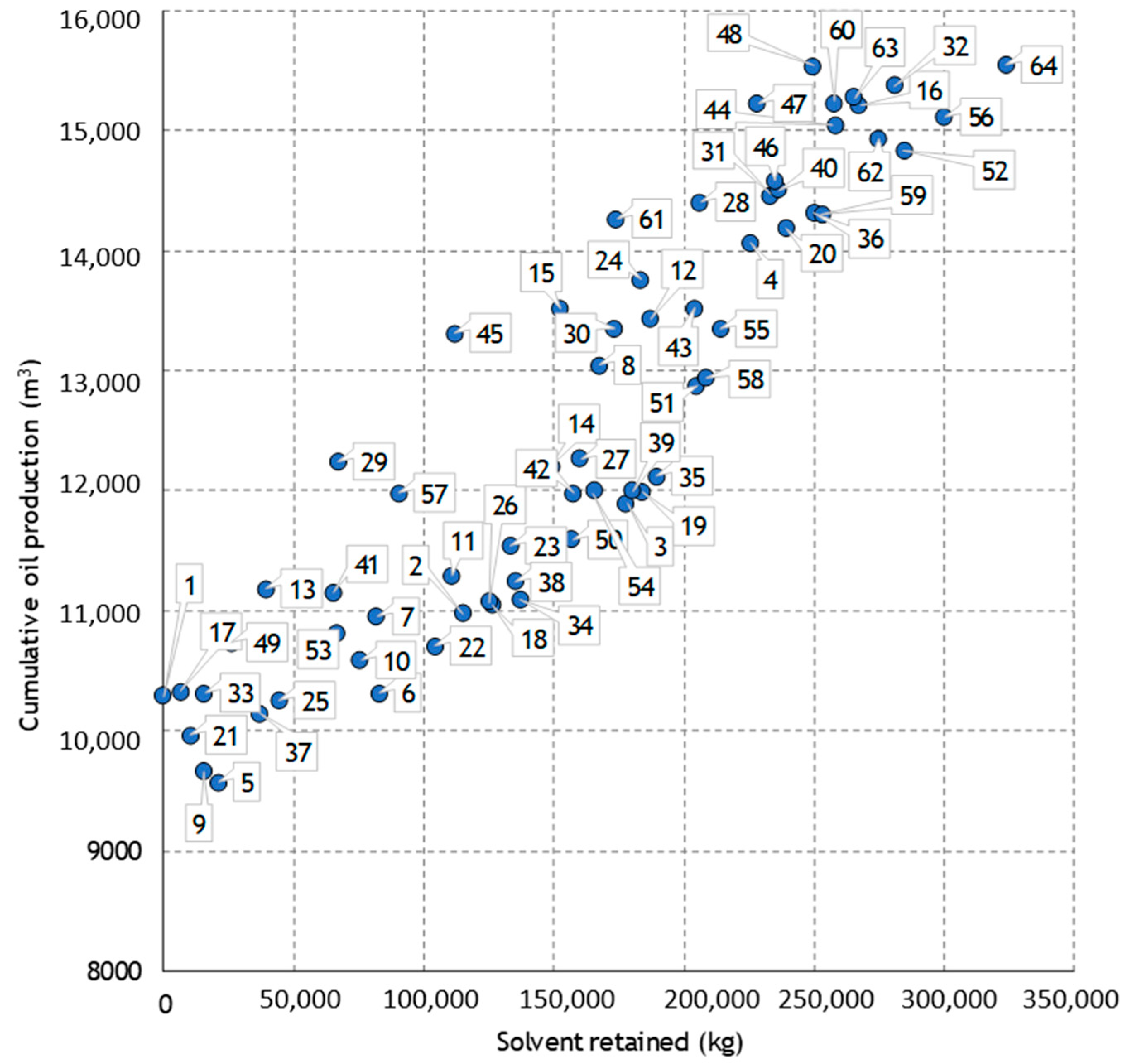
The results of this section are summarized in Figure 13, which shows a plot of the cumulative oil production for each case as a function of the mass of solvent that was retained in the reservoir. This was calculated as the difference between the total mass of solvent injected and the total mass of solvent that was produced with the oil. The numbers next to each dot represent the identifier for each simulation. The complete results can be found in Appendix A. The results in Appendix A show that the most favourable schedule is to have a short initial solvent injection followed by two long injection periods. A possible explanation for this is that the viscosity reduction is more strongly influenced by an increase in temperature than it is by an increase in the amount of solvent. Additionally, for some cases it can be noticed how the oil production is practically the same but the amount of solvent that was retained varies considerably. This indicates that the duration and timing of the solvent co-injection cycles can be used to improve the efficiency of the process in terms of the amount of solvent that was retained in the reservoir.
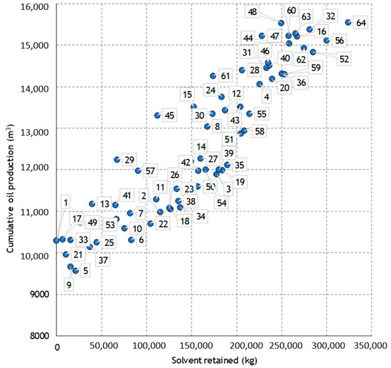
Figure 13.
Cumulative oil production in relation to the amount of solvent retained in the reservoir at the end of the simulation for cyclic ES-SAGD with different cycle’s duration. All cases contain hexane at 10% mole. The cycle’s duration for each case is reported in Table A1.
In Figure 13, there are four possible scenarios that relate the cumulative oil production with the retained solvent. The worst of these scenarios is having a process in which oil recovery is low and retained solvent is high. This would be an unfavorable process from an energy point of view and an unprofitable process because in most cases the solvents are more expensive than the oil that is produced. The scenario in which the oil production is high but the retained solvent is also high represents a continuous ES-SAGD process. If a continuous hexane co-injection at 10 mol% case is compared to the cases plotted in Figure 13, this case would be located at the top right corner since the amount of oil it recovered was 15,509 m3 and the amount of hexane that stayed in the reservoir was 623,000 kg. If the amount of cumulative oil production is low in comparison with the ES-SAGD case and the retained solvent is minimal then it would be similar to a SAGD process. Finally, the best scenario would be reaching a high production expending the least amount of solvent. The benefit of this would be having a more efficient process in terms of energy. Case 64 in Figure 13 has a cEOR of 10.8 GJ/m3 which is lower than 12.7 GJ/m3, the cEOR obtained in an ES-SAGD process using the same solvent at the same concentration. Case 48 has the same cumulative oil production of Case 64 but with an even lower cEOR (10.5 GJ/m3). The results presented in Figure 13 show that there might be a way of reproducing this scenario if the duration and timing of each cycle is modified.
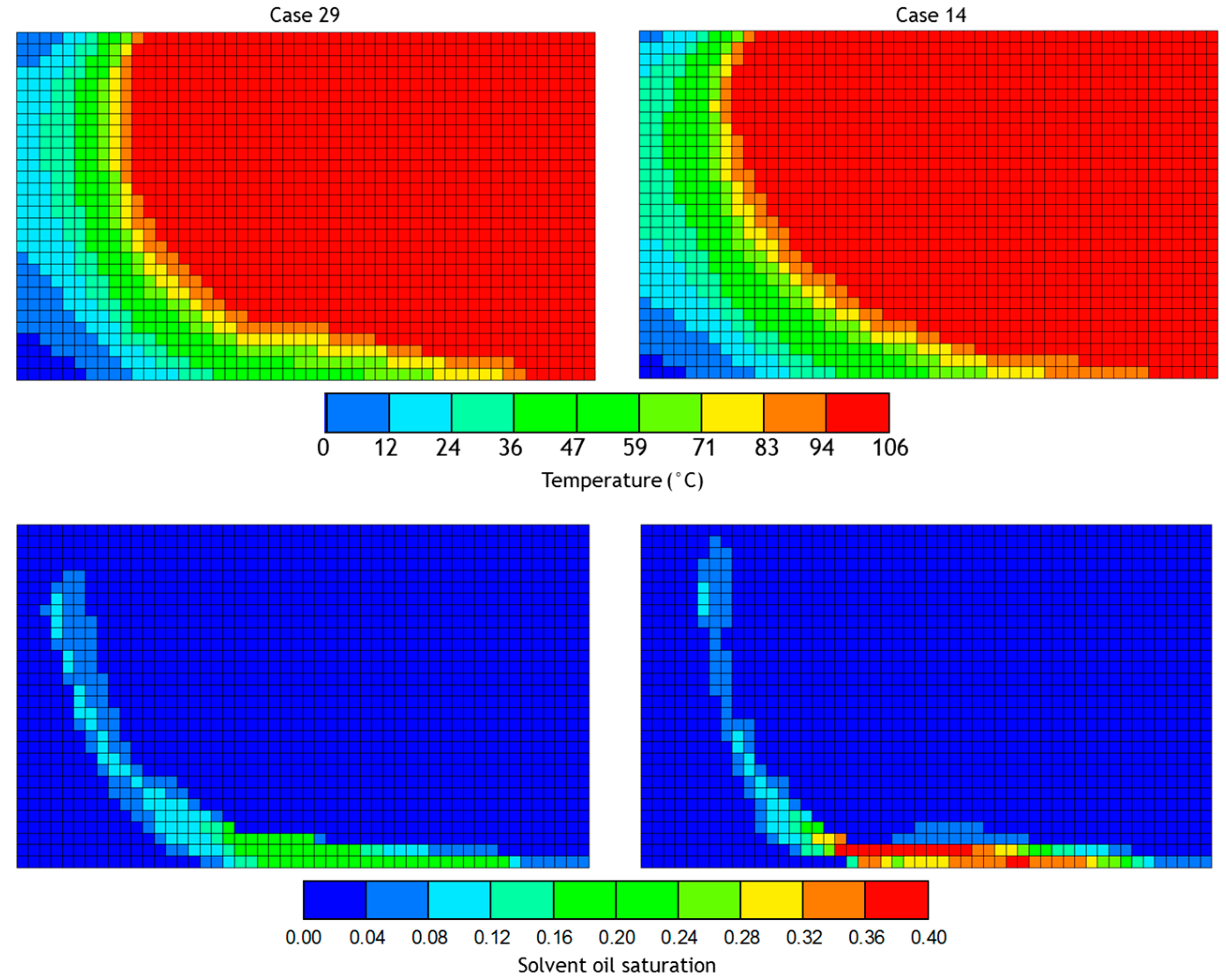
If two cases have a similar amount of oil production but one of them is leaving more solvent in the reservoir then, a possible explanation is that the final period of pure steam injection is not long enough to recover all the solvent that was injected in the previous cycles. Most of the cases shown in Figure 13, which recovered a similar amount of oil but with less retained solvent, only had solvent co-injection in the first two cycles. The final cycle in which the injection consisted of just steam allowed them to recover most of the solvent that was used. One example of this can be observed in the Cases 29 and 14. Both cases have 30 months of total solvent co-injection and, while the cumulative oil production of these cases is almost identical, Case 14 has an amount of solvent retained that is more than twice the amount of solvent that was retained in Case 29. The reason why in this case the solvent recovery was higher is related to the order in which the solvent was co-injected: Case 29 had more time at the end of the process to recover the solvent. Figure 14 shows the temperature distribution and solvent saturation in the oil the phase for both cases at the last time step. The shape of the steam chamber is practically identical between both cases which explains why the amount of oil that was drained is almost the same. However, the amount of solvent that is still at the reservoir at the end of the simulation varies significantly, which makes all the difference between both cases.

Figure 14.
Temperature and solvent saturation in oil phase for two cyclic ES-SAGD cases in which hexane at 10% mole was injected at different times. Although there is a subtle difference in the steam chamber size for both processes, it can be observed how there is more solvent in the oil phase in Case 14 at the end of the simulation.
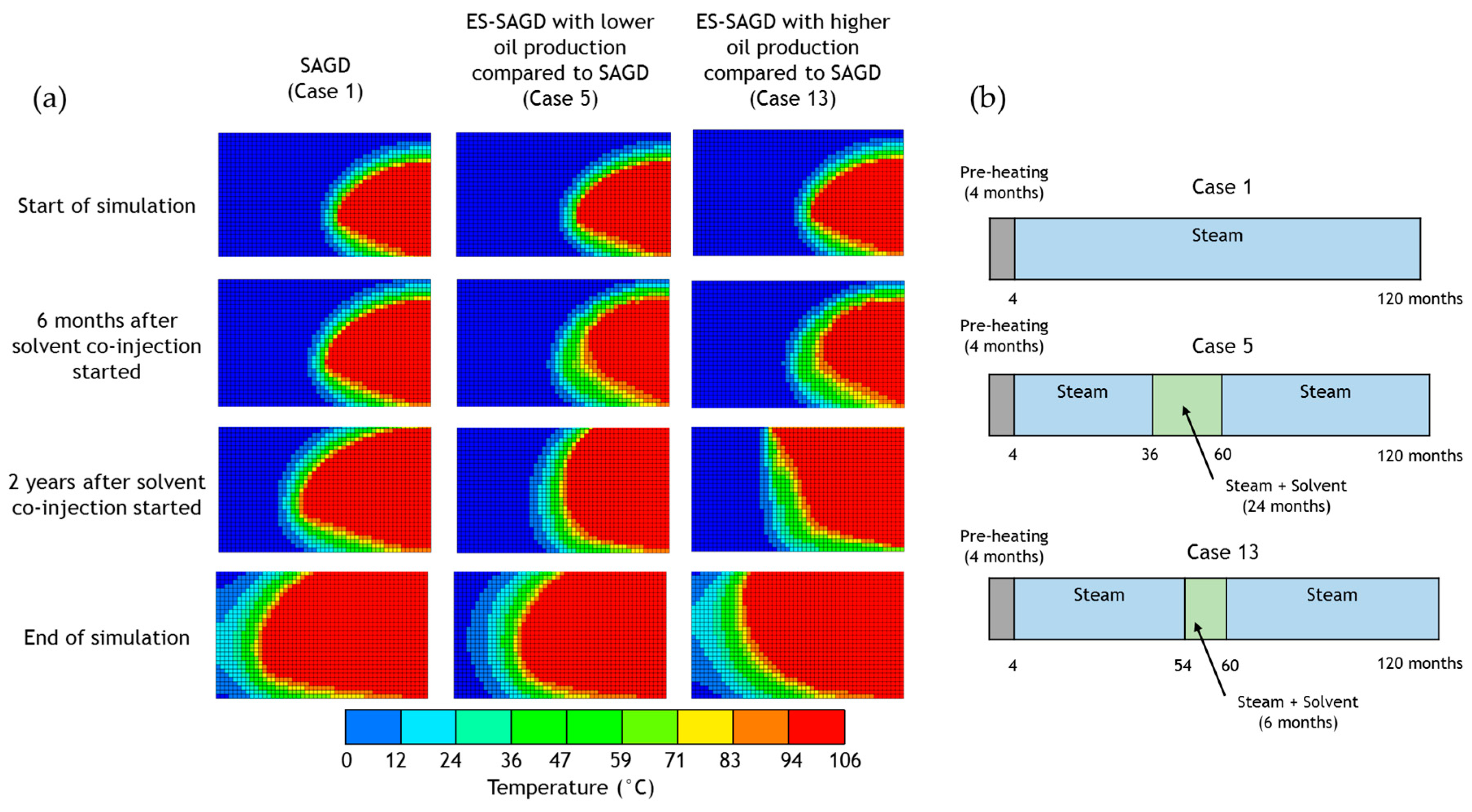
Appendix A and Figure 13 also show that, for some of the cases, the way in which the solvent is co-injected can even lead to a lower oil production than a pure steam injection case. One such case is investigated in Figure 15. Figure 15a shows the temperature distribution for a SAGD case without solvent co-injection (Case 1), a case in which the addition of the solvent led to a lower oil production (Case 5) and a case in which solvent co-injection increased the oil recovered (Case 13). In addition, Figure 15b contains a diagram that shows the moment at which the solvent was co-injected with the steam for each case.

Figure 15.
(a) Temperature distribution at four different moments during the simulation of three cases at which hexane at 10% mole was co-injected using cycles of different duration. (b) Timing and duration of the steam and solvent cycles for each case.
The only difference between Cases 5 and 13 is the duration of the solvent co-injection period. In both cases, there was only one co-injection period that started at the same time but that it had a duration of 24 months for Case 13 and six months for Case 5. At the moment in which the solvent co-injection started, the three cases in Figure 15 show similar temperature distributions. Six months later, there is a difference between the chamber shape for SAGD and the other two chambers. It is noted that in the solvent co-injection cases there is a thicker layer around the red area of the steam chamber which represents the solvent layer. The temperature distribution and chamber interface that are shown in these pictures relate to the moment at which solvent co-injection stopped for Case 5. Eighteen months later, when steam co-injection ends for Case 13, the chamber shape and interface positions for both cyclic ES-SAGD cases are considerably different. This is the moment at which the solvent co-injection stops for Case 13. It is important to note the difference of interfaces between both cyclic ES-SAGD cases at the moment when the solvent co-injection stops. For Case 5, the interface had not reached the top boundary of the model while for Case 13, the top section of the interface was at the model top boundary and it had a higher horizontal displacement than the rest of the interface. The last set of images show the temperature distribution at the end of the operation. The shape of the interface for Case 5 and SAGD are similar although for SAGD the steam chamber is bigger which explains why the oil production is higher. The interface position for Case 13 is different from the other cases particularly at the top section where it covers a bigger area leading to higher oil production than the SAGD case.
The results in the previous figures reveal that solvent co-injection could have a negative effect on final cumulative oil production due to the way in which the steam chamber grows and the shape of the interface. In ES-SAGD, the growth of the solvent layer is not uniform along the interface; this layer starts to thicken at the bottom of the chamber. This change in thickness alters the way in which the chamber expands making it grow considerably faster vertically rather than horizontally at the start of the process. After the chamber has reached the top of the model, it continues to move horizontally. On the contrary, in SAGD, although the chamber also grows vertically first and then horizontally, the difference between vertical and horizontal displacement of the steam chamber is subtler than in ES-SAGD. If a steam-solvent injection process is changed to a pure solvent injection process during the vertical expansion phase, then the depletion chamber will start to grow faster horizontally than vertically before having reached the top of the domain leaving some areas unaffected by the chamber.
3.4. Variations in the Mole Fraction and Duration of the Cycles
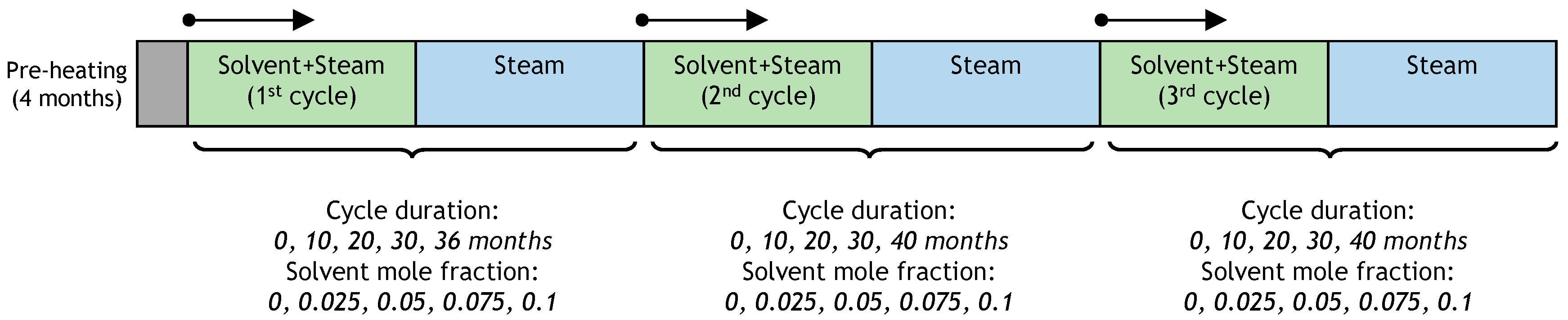
In these cases, the solvent mole fractions, durations of cycles, and start mode were changed. To do this, the operating period was divided into three main parts. Each part contained a steam-solvent cycle that could take a maximum value of 40 months and minimum value of zero months (which would convert this cycle to a pure steam cycle). In addition, the solvent mole fraction was changed from zero to 0.1 in each of the steam-solvent cycles. Figure 16 shows a graphical representation of the operating strategy. Due to the high number of possible combinations of all the parameters it was decided to test only a set of combinations and reach the best scenario through a workflow using the CMOST optimization package. In addition to this optimization algorithm, a MATLAB function that generated the wells’ schedule for each case was also used.
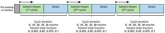
Figure 16.
Changes in the duration and solvent concentration for each of the steam-solvent cycles.
According to the results obtained in the previous section, if cyclic ES-SAGD is expected to reach the same cumulative oil productions of ES-SAGD while reducing the cEOR, it is necessary to avoid leaving a considerable amount of solvent in the reservoir. At the same time, it is important to inject just enough solvent to avoid the production of an oil phase that is composed mostly of solvent component. In the cases with changes in the duration of the cycles, it was noticed that longer cycles lead to higher cEOR values and do not necessarily imply higher oil productions. In these cases, the best performance was obtained by using a first steam-solvent cycle that was shorter than the rest of the cycles. This suggests that the addition of solvent at the start of the process may not be as beneficial as adding solvent at the end of the process if there is a period of pure steam injection after this cycle to recover the solvent.
Taking into account what was observed above, the initial point to start the optimizer was a case in which the first part consisted in a pure steam injection and the second and third parts involved solvent cycles that increased in duration and mole fraction. The optimizer was set to find the lowest cEOR but without reducing the highest cumulative oil production found in previous runs. The result of this process is shown in Figure 17. The first 36 months after the pre-heating period consists of steam injection followed by solvent co-injection of 0.075 mole fraction that is raised to 0.1 after 40 months. In the final stage, this mole fraction is kept for 30 months before switching to steam injection. The best case obtained in this final set of cases led to a cEOR of 10.1 GJ/m3 with oil production 15914 m3, which is slightly higher than cumulative production volumes reached in previous cases.

Figure 17.
Combination of cycle’s duration and mole fraction that led to the same amount of oil production with a lower cEOR.
Figure 18 shows a comparison between cumulative oil production obtained in the best case that was found through the optimization process and other cases. These cases are referred to different scenarios where the same solvent was injected continuously at different mole fractions during the same steam-solvent period that was used in the best case. The results show that the right combination of cycles’ duration and mole fractions can lead to improved results in terms of the cumulative oil production and, at the same time, increase the energy efficiency of the process that is measured through the cEOR.
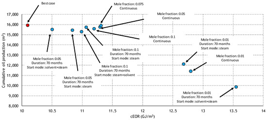
Figure 18.
Comparison between the best cyclic ES-SAGD cases and other cases where the solvent is added continuously to the steam or trough cycles of different duration. In all of these cases, hexane is used as solvent.
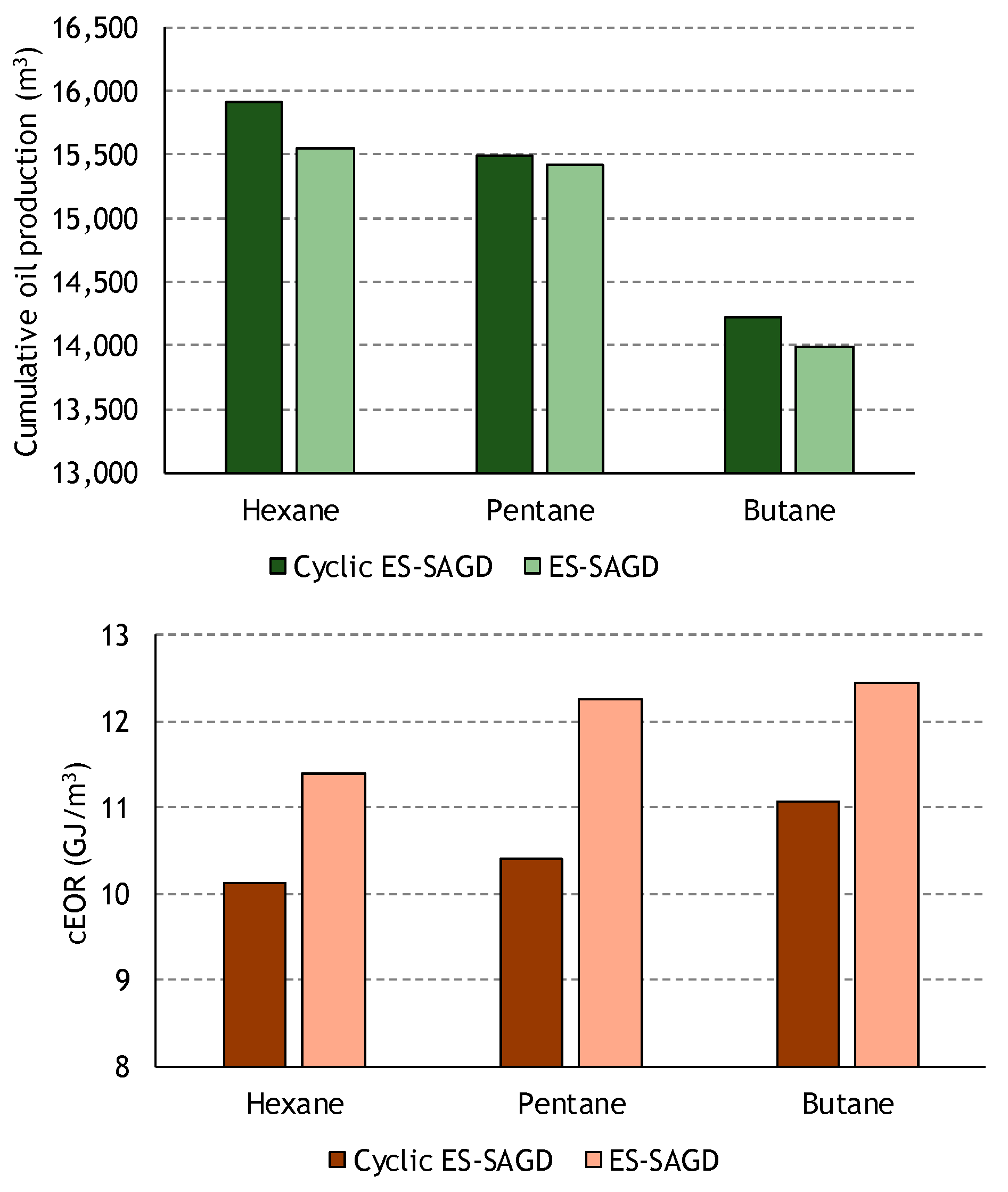
The above analysis that was performed using hexane was repeated for cases that included butane and pentane co-injection. Since the solvent-bitumen interaction leads to different combinations of cycles’ durations and solvent concentrations depending on the solvent that is used, it was necessary to determine the best case for the additional solvents. Figure 19 shows a comparison between cumulative oil production and cEOR for the best ES-SAGD cases and the cyclic ES-SAGD cases that were defined in this section. The cyclic ES-SAGD cases are showing better results in terms of oil production and cEOR. Although the differences in oil production are small, the comparison between cEOR values reveals differences that are always larger than 1 GJ/m3 compared to the ES-SAGD cases and even larger when compared to the SAGD case cEOR (13.4 GJ/m3). The differences between the results of the different solvents are related to the viscosity behavior of the solvent-bitumen mixture.

Figure 19.
Comparison in terms of cEOR and cumulative oil production for cyclic ES-SAGD and ES-SAGD cases using hexane, pentane, and butane.
The simulations that were presented in this section show that cyclic ES-SAGD can improve upon ES-SAGD if the duration of cycles and the solvent concentrations in each of them are chosen appropriately. Unfortunately, the impact that the duration of cycles and solvent concentration have in the performance of the reservoir cannot be generalized—each reservoir will have its own optimal duration of solvent co-injection and solvent mole fraction that will improve the way in which the steam chamber grows which, in turn, will define how much solvent is in contact with the oil and how much of this oil will finally move towards the production well.
It is important to mention that in a rigorous reservoir model with heterogeneous characteristics, the shape and growth of the steam chamber will be dictated not only by the fluid properties of both the oil and the injected the fluid but by the distribution of geological properties such as permeability and porosity. In addition to this, the presence of barriers or faults will also impact the movement of the fluids in the reservoir and, hence, the shape of the steam chamber. In these cases, a thorough geological description of the variation of properties in the reservoir, coupled with the numerical simulator is a better way of obtaining accurate predictions from the simulation process.
The heterogeneity in reservoir properties as well as in the grain size will also have an impact on the dispersion of the solvent as shown in a recent study by Liang et al. [35]. They concluded that solvent dispersion has a considerable effect as a dissipative process depending on the grain size of the reservoir. This will also modify the shape and growth of the steam chamber as well as the amount of oil that is affected by the solvent presence.
3.5. Preliminary Economic Analysis
In this section, cyclic ES-SAGD was compared with ES-SAGD and SAGD in terms of its net present value (NPV) at the end of 10 years of operation. This analysis contained approximate costs and prices for the solvent, oil and water. It is important to note that all the values that were used in this economic analysis are rough estimates, based on available data, and do not represent all the necessary input data for a complete economic analysis. One of the principal limitations of this analysis is that it does not consider any operational costs for any of the processes. The assumptions that were taken into consideration are the following:
- All processes are assumed to have the same initial investment; this component of the total cost was not taken into account for any of the cases.
- A constant average oil price is applied during the whole evaluation period.
- No additional cost for solvent co-injection besides the solvent cost.
- Amount of carbon dioxide emissions tax depends only on the amount of steam injected.
- Interest rate is 10%.
- It is assumed that 75% of the produced water is re-injected again as steam [36].
Table 3 shows the prices of oil, water, and solvent that were used in this analysis. The hexane and water prices were taken from Ghasemi and Whitson [37], which made a similar analysis for an ES-SAGD process, while the prices for butane and pentane are the one used by McWhinney [38].
Table 3.
Prices considered in the economic analysis.
The carbon tax that is considered is the one imposed by the Province of Alberta in 2016 that consists in CAD$30/tonne carbon dioxide. Considering the enthalpy of the injected steam and the stoichiometry of the combustion process of natural gas (methane), the amount of water injected was related with the amount of CO2 released. For this case, it was taken into account that the steam quality was 80% and the efficiency of the steam generation taken to be 75% [39]. If the relation between water injected and CO2 emitted is known then it is possible to estimate the taxes at each period and include them in the calculation. Figure 20 shows the relation between the cumulative SOR and the amount of CO2 released per volume of oil produced considering the steam enthalpy at 2500 kPa with 80% quality and a boiler efficiency of 75%.
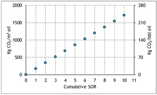
Figure 20.
Relation between the mass of carbon dioxide released per volume of oil produced and the cumulative steam-oil ratio.
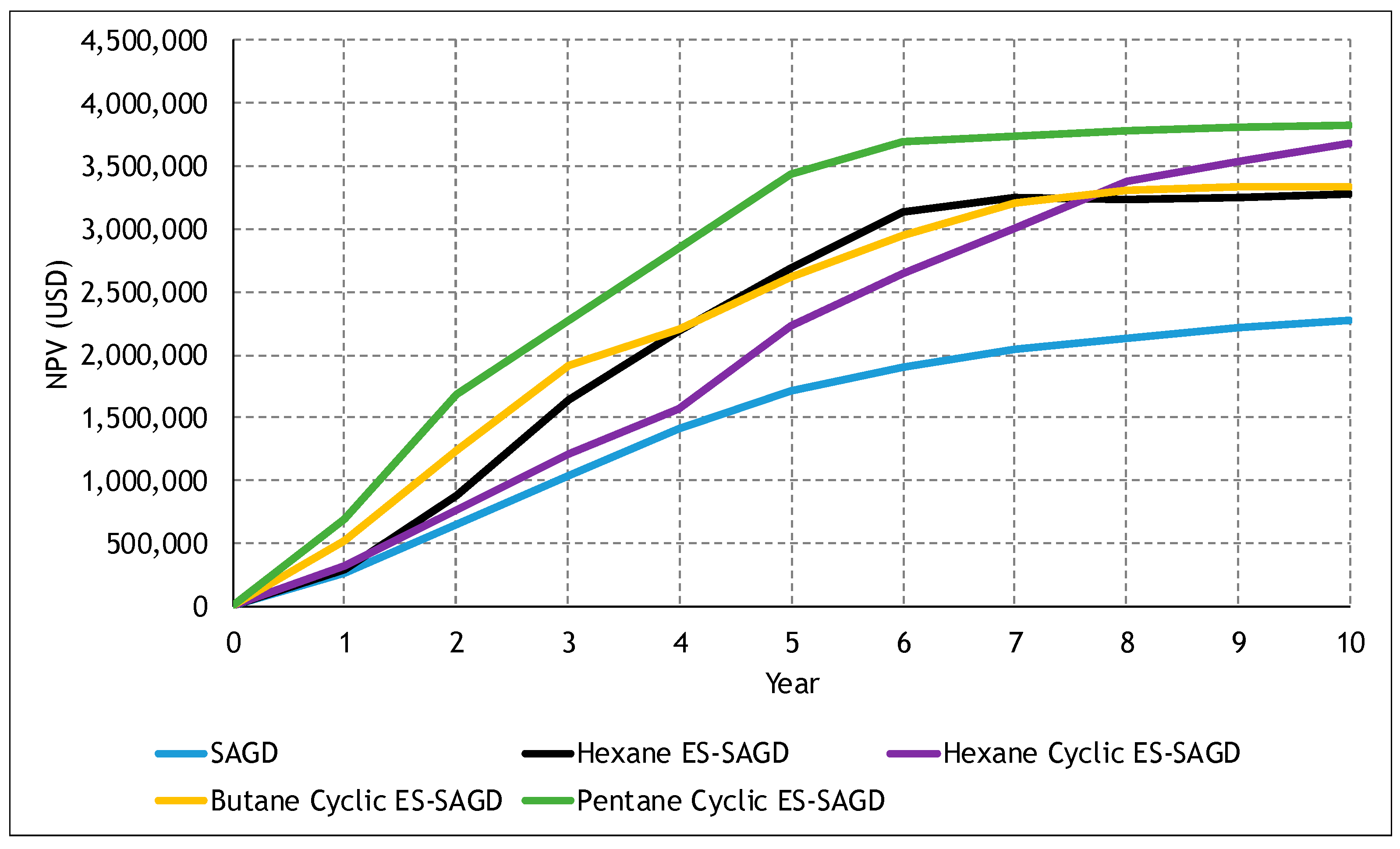
Figure 21 shows the NPV during the simulation period for the best hexane, pentane, and butane co-injection cases in terms of cumulative oil production and cEOR, and two additional scenarios: The continuous hexane co-injection at 10% mole and a SAGD case. The cases in which non-condensable gases where added to the steam are not being considered because in all these cases the final cumulative oil production was lower than the one obtained with SAGD. Figure 21 shows a similar NPV for all cases except the SAGD case where the NPV is considerably lower. Cyclic co-injection with pentane exhibits the best results in terms of the NPV at each of the years that were analyzed in the simulation period. This is due in part to the high cumulative oil production values that were achieved in this case, and also to the lower price of the pentane when compared to hexane. The best pentane co-injection case had a lower cumulative oil production and a higher cEOR than the best hexane co-injection case; however, because of the higher cash flows particularly at the beginning of the simulation, the NPVs of the pentane cyclic co-injection were always higher than the hexane case.
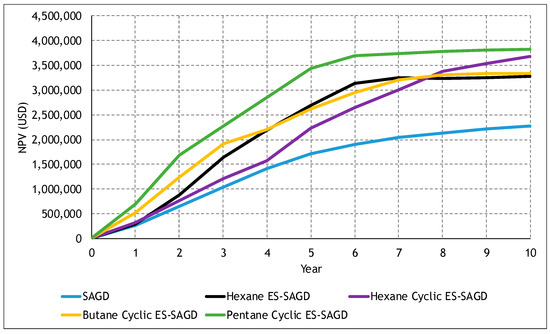
Figure 21.
NPV (Net present value) for multiple SAGD cases with solvent and cyclical solvent co-injection.
It is important to remember that the results that are shown in Figure 21 depend on the cumulative oil production for each case which in turn depends on the solvent-bitumen mixture viscosity data that was used in the simulation. As it was previously mentioned, this is a considerably important information that can affect the estimation of the final oil production and profitability of the process. The behavior of the bitumen-solvent mixture will directly impact the way in which the oil viscosity is reduced due to the dilution of the solvent. This will modify the amount of oil that is drained by the effect of gravity and that is eventually produced. In addition to this, the cost of the facilities and the operating expenses can also modify the results in terms of the NPV. These costs can change depending on the type of solvent that is used and the operating conditions. As it was mentioned at the beginning of this section, this is an important limitation of this study that should be addressed in a thorough economic analysis of SAGD or ES-SAGD processes.
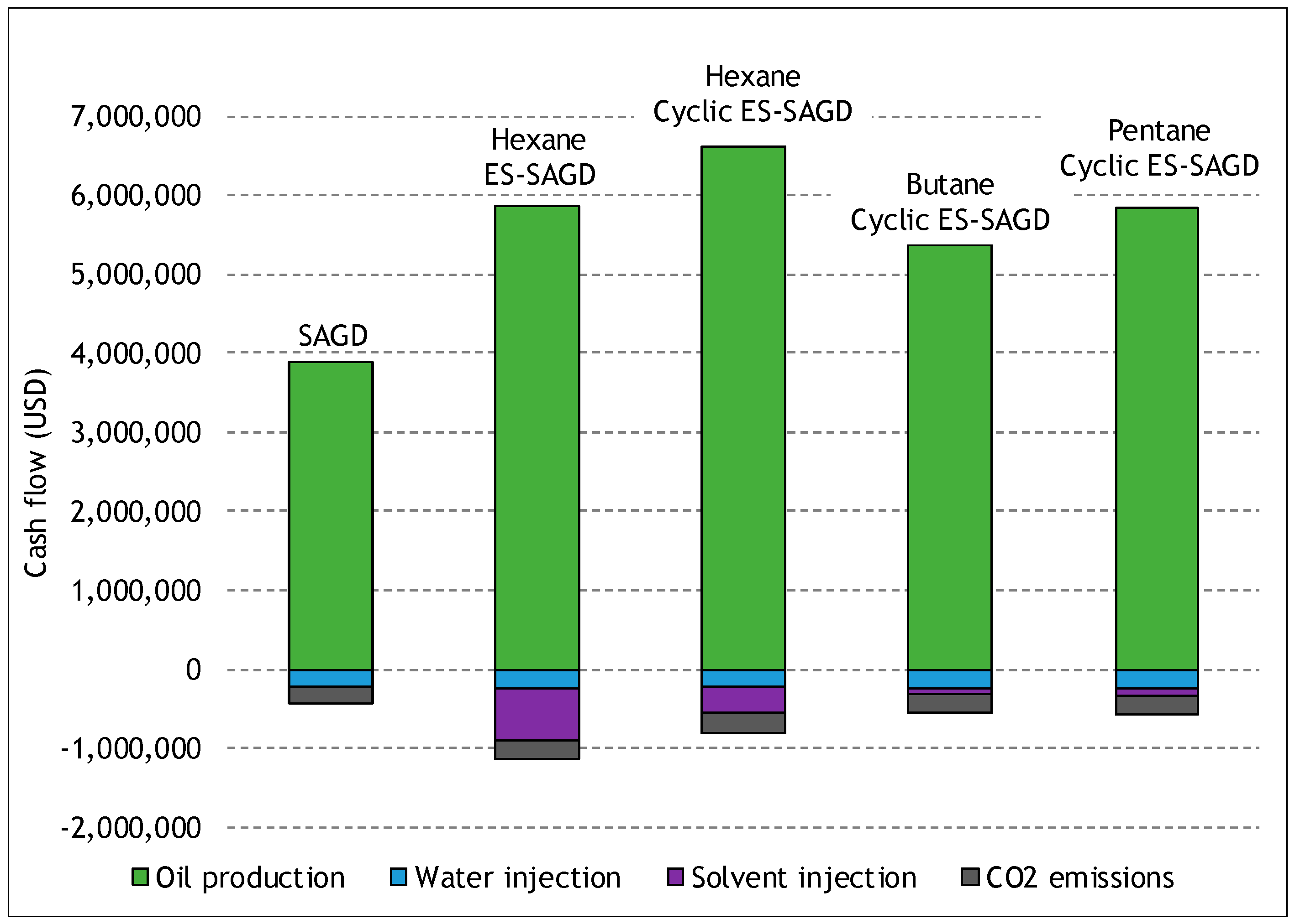
Figure 22 displays cumulative cash flows at the final year for each of the cases. The variations in the oil production income are directly related to the final oil cumulative production at each case. Regarding the expenses, it can be noticed how all cases have a similar negative cash flows related to the carbon dioxide emissions and water injection while the expenses related to the solvent injection are considerably different among all the cases.

Figure 22.
Cash flows after 10 years for each of the cases that were considered for the NPV analysis.
While there are no similar analyses of ES-SAGD for comparison, Giachetta et al. [40] performed an economical study of a SAGD process using actual production. Their study took into account operational costs and energy requirements from different elements of a SAGD operation. These costs, as well as the production data that comes from a SAGD process, were gathered from different literature references and, in some cases, assumed. One of their conclusions is that the influence of the capital cost and the oil price in the NPV is greater than the influence of the average natural gas cost, which is used to generate the injected steam. Although the study from Giachetta et al. [40] is not considering solvent co-injection with the steam, its results are important to understand the impact that the cost of the operation and facilities has on the profitability of an ES-SAGD process. In addition to this, the economic analysis is also affected by the volatility of oil prices which, should be carefully analyzed in a complete economic study of SAGD or ES-SAGD.
4. Conclusions
The most important aspect to consider from the results is that co-injecting the solvent in cycles instead of continuously could be beneficial for an ES-SAGD process not only from an energetic but also from an economic point of view. Although experimental studies and field tests have proven that the solvent retention in many ES-SAGD processes is low, the results are showing that with the right combination of cycles and solvent mole fractions, a cyclic ES-SAGD process could be able to achieve even less retention of solvent with the same amount of cumulative oil production. This would improve the efficiency and economics over that of the ES-SAGD process. The moment at which the solvent is injected with the steam and the period during which this injection takes place will affect the growth of the steam chamber as well as the velocity at which the chamber’s interface moves in the reservoir. This, in turn, will modify the reservoir area that interacts with the steam chamber and will consequently alter the final cumulative oil production and solvent retention. It is important to take into account that the duration and timing of the cycles and their solvent concentration needs to be determined for each reservoir and for each different type of solvent and oil. The performance of a cyclic ES-SAGD process is dependent not only in the characteristics of the steam-solvent cycles but also in the behavior of the solvent-bitumen mixture. Finally, it is necessary to point out that the results that were presented came from a simulation model that was a representation of half of the steam chamber that is formed in a confined homogeneous reservoir. The heterogeneity and size of each reservoir as well as the presence of multiple steam chambers can strongly affect the results and should be studied in future research.
Author Contributions
All three authors contributed significantly towards conceptualization, methodology, writing—original draft preparation and writing—review and editing. Funding acquisition and project administration were provided by M.C. and formal analysis was provided by D.M.J.
Funding
This research received no external funding.
Conflicts of Interest
The authors declare no conflict of interest.
Nomenclature
| Symbols | |
| AER | Alberta Energy Regulator |
| cEOR | Cumulative energy-oil ratio (GJ/m3) |
| cSOR | Cumulative steam-oil ratio |
| Heat capacity (J/(m3∙°C)) | |
| ES-SAGD | Expanding Solvent Steam Assisted Gravity Drainage |
| Permeability (md) | |
| P | Pressure (kPa) |
| Injection/production (m3) | |
| SAGD | Steam Assisted Gravity Drainage |
| Saturation | |
| Residual oil saturation to water | |
| Irreducible water saturation | |
| Residual oil saturation to gas | |
| Critical gas saturation | |
| Relative permeability of water at the residual oil saturation | |
| Relative permeability of oil at the irreducible water saturation | |
| Relative permeability of oil at the critical gas saturation | |
| Relative permeability of gas at the residual oil saturation | |
| Time (s) | |
| T | Temperature (° C) |
| Velocity (m/s) | |
| Molar fraction of component | |
| Axial axis in the reservoir (m) | |
| Greek letters | |
| Density (kg/m3) | |
| Viscosity (mPa.s) | |
| Molar density of component | |
| Porosity | |
| Thermal conductivity (J/(m∙day∙°C)) | |
Appendix A
Table A1.
Cumulative oil production and solvent retained for cyclic ES-SAGD cases with hexane at 10% mole and different cycle’s durations.
Table A1.
Cumulative oil production and solvent retained for cyclic ES-SAGD cases with hexane at 10% mole and different cycle’s durations.
| - | Cycle Duration (Months) | - | - | - | - | ||
|---|---|---|---|---|---|---|---|
| Case # | C1 | C2 | C3 | Prod Oil Cum (m3) | Solvent Injected (kg) | Solvent Produced (kg) | Solvent Retained (kg) |
| 1 | 0 | 0 | 0 | 10,295.1 | 10,295.1 | 0.0 | 0.0 |
| 2 | 0 | 0 | 6 | 10,981.9 | 10,981.9 | 864,979.2 | 749,778.3 |
| 3 | 0 | 0 | 12 | 11,891.6 | 11,891.6 | 2,275,017.8 | 2,097,119.4 |
| 4 | 0 | 0 | 24 | 14,065.3 | 14,065.3 | 6,442,483.5 | 6,217,169.5 |
| 5 | 0 | 6 | 0 | 9,571.3 | 9,571.3 | 1,331,663.4 | 1,310,617.4 |
| 6 | 0 | 6 | 6 | 10,317.0 | 10,317.0 | 2,231,307.0 | 2,148,552.3 |
| 7 | 0 | 6 | 12 | 10,954.2 | 10,954.2 | 3,543,453.0 | 3,461,502.0 |
| 8 | 0 | 6 | 24 | 13,048.6 | 13,048.6 | 7,490,470.0 | 7,323,091.0 |
| 9 | 0 | 12 | 0 | 9,672.0 | 9,672.0 | 3,579,740.5 | 3,564,531.5 |
| 10 | 0 | 12 | 6 | 10,589.2 | 10,589.2 | 4,459,617.0 | 4,384,056.5 |
| 11 | 0 | 12 | 12 | 11,287.4 | 11,287.4 | 5,757,756.0 | 5,646,824.5 |
| 12 | 0 | 12 | 24 | 13,434.8 | 13,434.8 | 9,808,053.0 | 9,620,728.0 |
| 13 | 0 | 24 | 0 | 11,183.1 | 11,183.1 | 7,364,007.0 | 7,324,700.0 |
| 14 | 0 | 24 | 6 | 12,209.3 | 12,209.3 | 8,324,493.0 | 8,175,437.5 |
| 15 | 0 | 24 | 12 | 13,521.7 | 13,521.7 | 9,898,629.0 | 9,746,301.0 |
| 16 | 0 | 24 | 24 | 15,210.0 | 15,210.0 | 14,327,243.0 | 14,060,176.0 |
| 17 | 6 | 0 | 0 | 10,318.9 | 10,318.9 | 1,323,151.1 | 1,316,655.5 |
| 18 | 6 | 0 | 6 | 11,052.8 | 11,052.8 | 2,186,149.5 | 2,059,767.3 |
| 19 | 6 | 0 | 12 | 11,990.1 | 11,990.1 | 3,512,744.5 | 3,328,661.5 |
| 20 | 6 | 0 | 24 | 14,192.6 | 14,192.6 | 7,682,517.0 | 7,443,213.0 |
| 21 | 6 | 6 | 0 | 9,963.0 | 9,963.0 | 2,568,191.3 | 2,557,917.3 |
| 22 | 6 | 6 | 6 | 10,706.0 | 10,706.0 | 3,512,527.0 | 3,408,078.0 |
| 23 | 6 | 6 | 12 | 11,545.2 | 11,545.2 | 4,826,919.5 | 4,693,732.0 |
| 24 | 6 | 6 | 24 | 13,759.9 | 13,759.9 | 8,827,237.0 | 8,643,938.0 |
| 25 | 6 | 12 | 0 | 10,255.1 | 10,255.1 | 4,753,401.0 | 4,709,194.0 |
| 26 | 6 | 12 | 6 | 11,081.3 | 11,081.3 | 5,704,733.0 | 5,579,794.5 |
| 27 | 6 | 12 | 12 | 12,270.3 | 12,270.3 | 7,145,290.0 | 6,985,219.5 |
| 28 | 6 | 12 | 24 | 14,407.5 | 14,407.5 | 11,403,264.0 | 11,197,006.0 |
| 29 | 6 | 24 | 0 | 12,246.5 | 12,246.5 | 8,745,387.0 | 8,678,411.0 |
| 30 | 6 | 24 | 6 | 13,354.8 | 13,354.8 | 9,786,386.0 | 9,613,213.0 |
| 31 | 6 | 24 | 12 | 14,466.0 | 14,466.0 | 11,266,536.0 | 11,033,722.0 |
| 32 | 6 | 24 | 24 | 15,379.6 | 15,379.6 | 15,375,053.0 | 15,093,860.0 |
| 33 | 12 | 0 | 0 | 10,316.6 | 10,316.6 | 3,183,613.5 | 3,167,999.8 |
| 34 | 12 | 0 | 6 | 11,092.5 | 11,092.5 | 4,031,415.5 | 3,894,124.0 |
| 35 | 12 | 0 | 12 | 12,122.0 | 12,122.0 | 5,318,220.0 | 5,128,918.5 |
| 36 | 12 | 0 | 24 | 14,316.4 | 14,316.4 | 9,468,955.0 | 9,218,765.0 |
| 37 | 12 | 6 | 0 | 10,142.2 | 10,142.2 | 4,307,624.5 | 4,270,664.0 |
| 38 | 12 | 6 | 6 | 11,243.3 | 11,243.3 | 5,189,320.5 | 5,054,023.5 |
| 39 | 12 | 6 | 12 | 12,002.4 | 12,002.4 | 6,437,088.5 | 6,257,068.0 |
| 40 | 12 | 6 | 24 | 14,511.0 | 14,511.0 | 10,810,966.0 | 10,574,430.0 |
| 41 | 12 | 12 | 0 | 11,147.6 | 11,147.6 | 6,315,293.0 | 6,250,003.0 |
| 42 | 12 | 12 | 6 | 11,975.1 | 11,975.1 | 7,270,113.0 | 7,112,757.0 |
| 43 | 12 | 12 | 12 | 13,520.7 | 13,520.7 | 8,908,871.0 | 8,704,568.0 |
| 44 | 12 | 12 | 24 | 15,054.0 | 15,054.0 | 13,216,059.0 | 12,957,738.0 |
| 45 | 12 | 24 | 0 | 13,316.6 | 13,316.6 | 10,519,744.0 | 10,408,047.0 |
| 46 | 12 | 24 | 6 | 14,591.7 | 14,591.7 | 11,612,288.0 | 11,377,263.0 |
| 47 | 12 | 24 | 12 | 15,229.9 | 15,229.9 | 13,131,943.0 | 12,903,704.0 |
| 48 | 12 | 24 | 24 | 15,537.9 | 15,537.9 | 16,620,156.0 | 16,370,431.0 |
| 49 | 24 | 0 | 0 | 10,735.7 | 10,735.7 | 7,623,278.0 | 7,597,202.0 |
| 50 | 24 | 0 | 6 | 11,596.0 | 11,596.0 | 8,471,010.0 | 8,314,041.5 |
| 51 | 24 | 0 | 12 | 12,870.3 | 12,870.3 | 9,743,723.0 | 9,538,830.0 |
| 52 | 24 | 0 | 24 | 14,833.6 | 14,833.6 | 14,040,197.0 | 13,755,489.0 |
| 53 | 24 | 6 | 0 | 10,820.9 | 10,820.9 | 8,654,386.0 | 8,587,784.0 |
| 54 | 24 | 6 | 6 | 12,001.2 | 12,001.2 | 9,576,025.0 | 9,410,692.0 |
| 55 | 24 | 6 | 12 | 13,353.1 | 13,353.1 | 11,051,944.0 | 10,837,979.0 |
| 56 | 24 | 6 | 24 | 15,119.4 | 15,119.4 | 15,336,156.0 | 15,035,886.0 |
| 57 | 24 | 12 | 0 | 11,982.1 | 11,982.1 | 10,457,010.0 | 10,366,752.0 |
| 58 | 24 | 12 | 6 | 12,941.9 | 12,941.9 | 11,409,638.0 | 11,200,851.0 |
| 59 | 24 | 12 | 12 | 14,308.4 | 14,308.4 | 13,009,759.0 | 12,756,603.0 |
| 60 | 24 | 12 | 24 | 15,232.3 | 15,232.3 | 17,005,370.0 | 16,747,578.0 |
| 61 | 24 | 24 | 0 | 14,266.9 | 14,266.9 | 14,654,803.0 | 14,480,880.0 |
| 62 | 24 | 24 | 6 | 14,932.0 | 14,932.0 | 15,741,781.0 | 15,466,795.0 |
| 63 | 24 | 24 | 12 | 15,279.7 | 15,279.7 | 16,986,908.0 | 16,721,624.0 |
| 64 | 24 | 24 | 24 | 15,554.8 | 15,554.8 | 20,028,112.0 | 19,704,138.0 |
| 49 | 24 | 0 | 0 | 10,295.1 | 10,735.7 | 7,623,278.0 | 7,597,202.0 |
References
- Statistics|World—Oil Product Consumptions. U.S. Energy Information Administration (EIA). International Energy Statistics. Available online: https://www.iea.org/statistics/ (accessed on 5 January 2019).
- BP Statistical Review of World Energy; BP: London, UK, 2018.
- Butler, R. Steam Assisted Gravity Drainage. In Thermal Recovery of Oil and Bitumen, 1st ed.; GravDrain: Calgary, AB, Canada, 1991; pp. 285–359. [Google Scholar]
- Moore, R.G.; Laureshen, C.J.; Ursenbach, M.G.; Mehta, S.A.; Belgrave, J.D.M. A Canadian Perspective on In Situ Combustion. J. Can. Petrol. Technol. 1999, 38. [Google Scholar] [CrossRef]
- Farouq Ali, S.M.; Bayestehparvin, B. Electrical Heating—Doing the same thing over and over again. In Proceedings of the SPE Canada Heavy Oil Technical Conference, Calgary, AB, Canada, 13–14 March 2018. [Google Scholar]
- Butler, R. The steam and Gas Push (SAGP). J. Can. Petrol. Technol. 1999, 38, 54–61. [Google Scholar] [CrossRef]
- Shen, C. Numerical Investigation of SAGD Process Using a Single Horizontal Well. In Proceedings of the SPE International Conference on Horizontal Well Technology, Calgary, AB, Canada, 1–4 November 1998. [Google Scholar]
- Stalder, J. Cross SAGD (XSAGD)—An Accelerated Bitumen Recovery Alternative. In Proceedings of the SPE International Thermal Operations and Heavy Oil Symposium, Calgary, AB, Canada, 1–3 November 2005. [Google Scholar]
- Nasr, T.; Beaulieu, G.; Golbeck, H.; Heck, G. Novel Expanding Solvent-SAGD Process “ES-SAGD”. J. Can. Petrol. Technol. 2003, 42, 13–16. [Google Scholar] [CrossRef]
- Risk Assessment of Solvent Injection Processes; Alberta Energy Regulator: Calgary, AB, Canada, 2018.
- Gates, I.; Chakrabarty, N. Design of the Steam and Solvent Injection Strategy in Expanding Solvent Steam-Assisted Gravity Drainage. J. Can. Petrol. Technol. 2008, 47, 12–20. [Google Scholar] [CrossRef]
- Zhao, L. Steam Alternating Solvent Process. In Proceedings of the SPE International Thermal Operations and Heavy Oil Symposium and Western Regional Meeting, Bakersfield, CA, USA, 16–18 March 2004; pp. 185–190. [Google Scholar]
- Butler, R.; Mokrys, I. A new process (VAPEX) for recovering heavy oils using hot water and hydrocarbon vapour. J. Can. Petrol. Technol. 1991, 30, 97–106. [Google Scholar] [CrossRef]
- CMG. Winprop User Manual; Computer Modelling Group: Calgary, AB, Canada, 2017. [Google Scholar]
- Zhang, Y.; Hu, J.; Zhang, Q. Simulation Study of CO2 Huff-n-Puff in Tight Oil Reservoirs Considering Molecular Diffusion and Adsorption. Energies 2019, 12, 2136. [Google Scholar] [CrossRef]
- Janiga, D.; Czarnota, R.; Stopa, J.; Wojnarowski, P. Huff and puff process optimization in micro scale by coupling laboratory experiment and numerical simulation. Fuel 2018, 224, 289–301. [Google Scholar] [CrossRef]
- Jorshari, K.; O’Hara, B. A New SAGD Well Pair Placement; a Field Case Review. In Proceedings of the Canadian Unconventional Resources Conference, Calgary, AB, Canada, 15–17 November 2011. [Google Scholar]
- Tamer, M.; Gates, I.D. Impact of Different SAGD Well Configurations (Dover SAGD Phase B Case Study). In Proceedings of the 10th Canadian International Petroleum Conference, Calgary, AB, Canada, 16–18 June 2009. [Google Scholar]
- CMG. STARS User Manual; Computer Modelling Group: Calgary, AB, Canada, 2017. [Google Scholar]
- Shin, H.; Polikar, M. Fast-SAGD application in the Alberta Oil Sands Area. J. Can. Petrol. Technol. 2006, 45, 46–53. [Google Scholar] [CrossRef]
- Rabiei, F., M. Mathematical Modeling of Steam-Solvent Gravity Drainage of Heavy Oil and Bitumen in Porous Media. Ph.D. Thesis, University of Calgary, Calgary, AB, Canada, 2013. [Google Scholar]
- Salama, D.; Kantzas, A. Monitoring of Diffusion of Heavy Oils with Hydrocarbon Solvents in the Presence of Sand. In Proceedings of the SPE International Operations and Heavy Oil Symposium, Calgary, AB, Canada, 1–3 November 2005. [Google Scholar]
- Gates, I. Oil phase viscosity behavior in Expanding-Solvent Steam-Assisted Gravity Drainage. J. Petrol. Sci. Eng. 2007, 59, 123–134. [Google Scholar] [CrossRef]
- Strauz, O.; Lown, E. Geology of the Alberta Bitumen and Heavy Oil Deposits. In The Chemistry of Alberta Oil Sands, Bitumens and Heavy Oils, 1st ed.; Alberta Energy Research Institute: Calgary, AB, Canada, 2003; pp. 21–26. [Google Scholar]
- Pedersen, K.; Fredenslund, A.; Christensen, P. Viscosity of Crude Oils. Chem. Eng. Sci. 1984, 39, 1011–1016. [Google Scholar] [CrossRef]
- Nourozieh, H.; Kariznovi, M.; Abedi, J. Viscosity measurement and modeling for mixtures of Athabasca bitumen/hexane. J. Petrol. Sci. Eng. 2005, 129, 159–167. [Google Scholar] [CrossRef]
- Nourozieh, H.; Kariznovi, M.; Abedi, J. Viscosity Measurement and Modeling for Mixtures of Athabasca Bitumen/n-Pentane at Temperatures up to 200 °C. SPE J. 2005, 170252, 226–238. [Google Scholar] [CrossRef]
- Nourozieh, H.; Kariznovi, M.; Abedi, J. Solubility of n-Butane in Athabasca Bitumen and Saturated Densities and Viscosities at Temperatures up to 200° C. SPE J. 2017, 180927, 94–102. [Google Scholar] [CrossRef]
- Nourozieh, H.; Kariznovi, M.; Abedi, J. Experimental and modeling studies of phase behavior for propane/Athabasca bitumen mixtures. Fluid Phase Equilib. 2015, 397, 37–43. [Google Scholar] [CrossRef]
- Nourozieh, H.; Kariznovi, M.; Abedi, J. Vapor-Liquid Equilibrium of Bitumen-Ethane Mixtures for three Athabasca Bitumen Samples. J. Chem. Eng. Data 2017, 62, 2198–2207. [Google Scholar]
- Nourozieh, H.; Kariznovi, M.; Abedi, J. Measurement and Modeling of Solubility and Saturated-Liquid Density and Viscosity for Methane/Athabasca-Bitumen Mixtures. SPE J. 2016, 174558, 180–189. [Google Scholar] [CrossRef]
- Haddadnia, A.; Zirrahi, M.; Hassanzadeh, H.; Abedi, J. Solubility and thermo-physical properties measurement of CO2 and N2—Athabasca bitumen samples. J. Petrol. Sci. Eng. 2017, 154, 277–283. [Google Scholar] [CrossRef]
- Bahadori, A.; Vuthaluru, H.B.; Tade, M.O.; Mokhatab, S. Predicting Water-Hydrocarbon Systems Mutual Solubility. Chem. Eng. Technol. 2008, 31, 1743–1747. [Google Scholar] [CrossRef]
- Zirrahi, M.; Hassanzadeh, H.; Abedi, J.; Moshfeghian, M. Prediction of solubility of CH4, C2H6, CO2, N2 and CO in bitumen. Can. J. Chem. Eng. 2014, 92, 563–572. [Google Scholar] [CrossRef]
- Liang, Y.; Wen, B.; Hesse, M.; DiCarlo, D. Effect of Dispersion on Solutal Convection in Porous Media. Geophys. Res. Lett. 2018, 45, 9690–9698. [Google Scholar] [CrossRef]
- Water Use Performance. Alberta Energy Regulator. Available online: https://www.aer.ca/protecting-what-matters/holding-industry-accountable/industry-performance/water-use-performance (accessed on 5 January 2019).
- Ghasemi, M.; Whitson, C. Numerical investigation and integrated optimization of Solvent-SAGD process. In Proceedings of the International Petroleum Technology Conference, Kuala Lumpur, Malaysia, 10–12 December 2014. [Google Scholar]
- McWhinney, R. Process Efficiencies of Unconventional Oil and Gas; Canadian Research Institute: Calgary, AB, Canada, 2015; p. 147. [Google Scholar]
- Gates, I.; Larter, S. Energy efficiency and emissions intensity of SAGD. Fuel 2014, 115, 706–713. [Google Scholar] [CrossRef]
- Giachetta, G.; Leporini, M.; Marchetti, B. Economic and environmental analysis of a Steam Assisted Gravity Drainage (SAGD) facility for oil recovery from Canadian oil sands. Appl. Energy 2015, 142, 1–9. [Google Scholar] [CrossRef]


© 2019 by the authors. Licensee MDPI, Basel, Switzerland. This article is an open access article distributed under the terms and conditions of the Creative Commons Attribution (CC BY) license (http://creativecommons.org/licenses/by/4.0/).