Mechanistic Characteristics of Double Dominant Frequencies of Acoustic Emission Signals in the Entire Fracture Process of Fine Sandstone

Abstract

To determine the intrinsic relationship between the acoustic emission (AE) phenomenon and the fracture pattern pertaining to the entire fracture process of rock, the present paper proposed a multi-dimensional spectral analysis of the AE signal released during the entire process. Some uniaxial compression AE tests were carried out on the fine sandstone specimens, and the axial compression stress–strain curves and AE signal released during the entire fracture process were obtained. In order to deal with tens of thousands of AE data efficiently, a subroutine was programmed in MATLAB. All AE waveforms of the tests were denoised by wavelet threshold firstly. The fast Fourier transform (FFT) and wavelet packet transform (WPT) were applied to the denoised waveforms to obtain the dominant frequency, amplitude, fractal, and frequency band energy ratio distribution. The results showed that the AE signal in the entire fracture process of fine sandstone had a double dominant frequency band of the low and high-frequency bands, which can be subdivided into low-frequency low-amplitude, high-frequency low-amplitude, high-frequency high-amplitude, and low-frequency high-amplitude signals, according to the magnitude. The low-frequency amplitude relevant fractal dimension and the high-frequency amplitude relevant fractal dimension each had turning points that corresponded to significant decreases in the middle and end stages of loading, respectively. The frequency band energy was mainly concentrated in the range of 0–187.5 kHz, and the energy ratios of some bands had different turning points, which appeared before the complete failure of the rock. It is suggested that the multi-dimensional spectral analysis may understand the failure mechanism of rock better.

1. Introduction

The fracture process of rock material is consistent with the evolutionary process of its internal microcracks. The initiation and propagation of microcracks cause stress relaxation, which is the sudden release of partially stored energy in the form of a stress wave. This release results in an acoustic emission (AE) phenomenon [1,2], which can quantitatively describe the internal lattice dislocation or microcrack propagation and the evolution of rock during its deformation under load; moreover, this phenomenon can, to some extent, reflect the energy release and damage level during the fracture process. AE is one of the effective tools to study the mechanism of rock fractures [3,4,5].

The current processing methods for an AE signal obtained in a laboratory can be mainly divided into two categories: One pertains to the use of the simplified waveform characteristic parameters, such as the ring-down count, event rate, energy rate, cumulative number of events, and accumulated energy, to represent the signal characteristics for processing and analysis [6,7,8]. Farahat and Ohtsu’s [9] research showed that the plastic damage of concrete under uniaxial compression is positively correlated with the activity of an AE signal. Bagde and Petros [10] found that under dynamic cyclic loading, the energy release of rock decreases with the increase of loading frequency. Moradian et al. [11] revealed that the number and energy of acoustic emission hits were related to the number of cracks and the magnitude of crack events, respectively. The other category of methods involves performing a fast Fourier transform (FFT) or wavelet packet transform (WPT) directly on the waveform to analyze the corresponding spectral characteristics. AE waveform signals possess rich information such as the rock stress state, change in the microstructure, and their combined characteristics, which have attracted wide research attention [12,13,14,15]. Ji et al. [16] studied the frequency characteristics of AE signals in different stages of uniaxial compression and the fracture of granite, and showed that the dominant frequencies of the AE signal occurred mainly in the plastic failure stage and major fracture stages. Morgan et al. [17] revealed the variation trends of the dominant frequency of the high- and low-frequency channels. Zhao et al. [18] revealed that the energy percentage of the characteristic band at the Kaiser effect point of sandstone is greater than that at the points adjacent to the Kaiser effect point. Lai et al. [19] analyzed the pattern of variation of the energy ratio at the low-frequency band of a rock-like material with the loading time. These research results helped improve our understanding of the characteristics of AE signals during the rock damage evolution process. It should be noted that most of the existing analyses were conducted choosing representative AE waveforms from an AE energy accumulation curve to analyze the rock fracture mechanism [15]. However, the number of AE waveforms released by a rock during deformation under load is of the order of tens of thousands, which corresponds to an enormous amount of generated data. As a result, the AE waveforms selected for analysis in the abovementioned studies are slightly under-representative. To address this problem and to further demonstrate the evolution pattern of the spectral characteristics of AE signals during the rock damage evolution process, it is necessary to comprehensively analyze the spectral characteristics of all AE waveforms generated in the entire process.

On this basis, in this study, a uniaxial compression AE test of fine sandstone was carried out. Each AE waveform released during the entire process of rock fracture was denoised and subjected to FFT and WPT to acquire the spectral characteristics and the distribution of the energy ratio of the AE signal band in different failure stages. The mechanism for the dominant frequencies of the AE signal and the distribution characteristics of the variation in band energy with stress were investigated. Meanwhile, the relevant fractal dimension of the AE signal amplitude was calculated and analyzed based on the fractal theory to determine the intrinsic relationship between the mechanical evolution process and the AE process.

2. Test and Data Processing

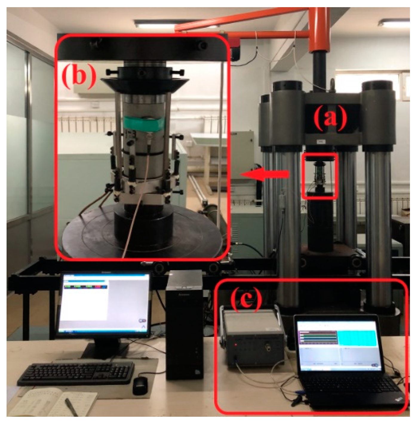
2.1. Outline of the Test

The test system included a SAS-2000 uniaxial testing machine and a SAEU2S AE monitoring system with a sampling frequency of 1000 kHz, sampling length (number of points) of 2048, preamplifier gain of 40 dB, and threshold value of 40 dB. The analog-to-digital converter (ADC) model of an AE monitoring system is PA I broadband, gain 40 dB (±1 dB) (available bits, resolution), maximum output V_pp >20 V, and maximum input V_pp >200 mV. In the test, a rock extensometer configured in the testing machine was used to collect the strain, and the axial equal displacement control mode is adopted. In the loading direction, a preload of 2 kN was applied. The sampling time of each system is synchronized after fully contacting the pressure end of the specimen with the testing machine. Then, the axial displacement control method with a loading rate of 0.05 mm/min was employed until the complete failure of the specimen. The test system is shown in Figure 1.

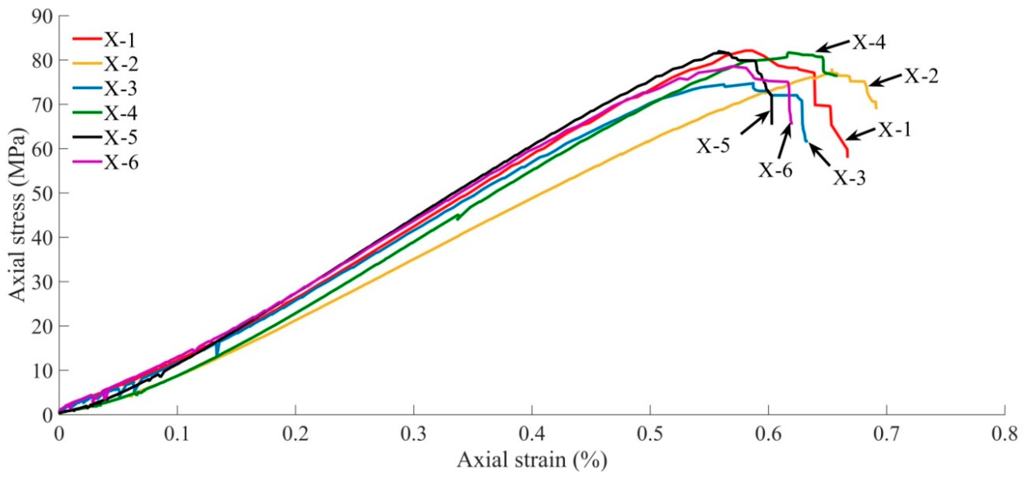
2.2. Basic Characteristic Mechanical Parameters of Specimens

The diameter of the specimen is 50 mm with a height of 100 mm. The two compression-bearing ends of the specimen were carefully ground to ensure that the unevenness of both ends was controlled within an error of 0.05 mm, and the end face was perpendicular to the axis within an error of less than 0.25°. The processed specimens were numbered sequentially as X-1 through X-6, and the detailed information is provided in

Table 1. Comparison basic physical and mechanical parameters of specimens.

Specimen Number	Diameter (mm)	Height (mm)	Loading Time (s)	Uniaxial Compressive Strength (MPa)	AE Waveform Quantity (pcs)
X-1	48.86	100.16	442.6	82.12	54,817
X-2	48.78	100.18	443.2	78.09	40,755
X-3	48.90	100.26	448.3	74.72	46,387
X-4	48.74	100.20	446.6	81.68	45,560
X-5	48.82	100.22	447.6	81.98	49,612
X-6	48.80	100.18	447.4	78.57	38,250

. Figure 2 shows the axial stress–strain curve of each specimen.

2.3. Data Processing

Table 1 presents all the AE waveforms released during the entire fracture process of the specimen. All AE waveforms were denoised by wavelet threshold (choosing db3 wavelet of Daubechies wavelet family as wavelet base, matching the Heursure threshold rule and soft threshold method) [20]. In order to improve the efficiency of data processing, a subroutine was programmed in MATLAB to first perform wavelet threshold denoising, and later FFT and the WPT were applied to the denoised waveforms to obtain the dominant frequency, amplitude, and frequency band energy ratio distribution, which are combined with the times and axial stress states recorded in the uniaxial compression test to obtain the complete test data for all specimens.

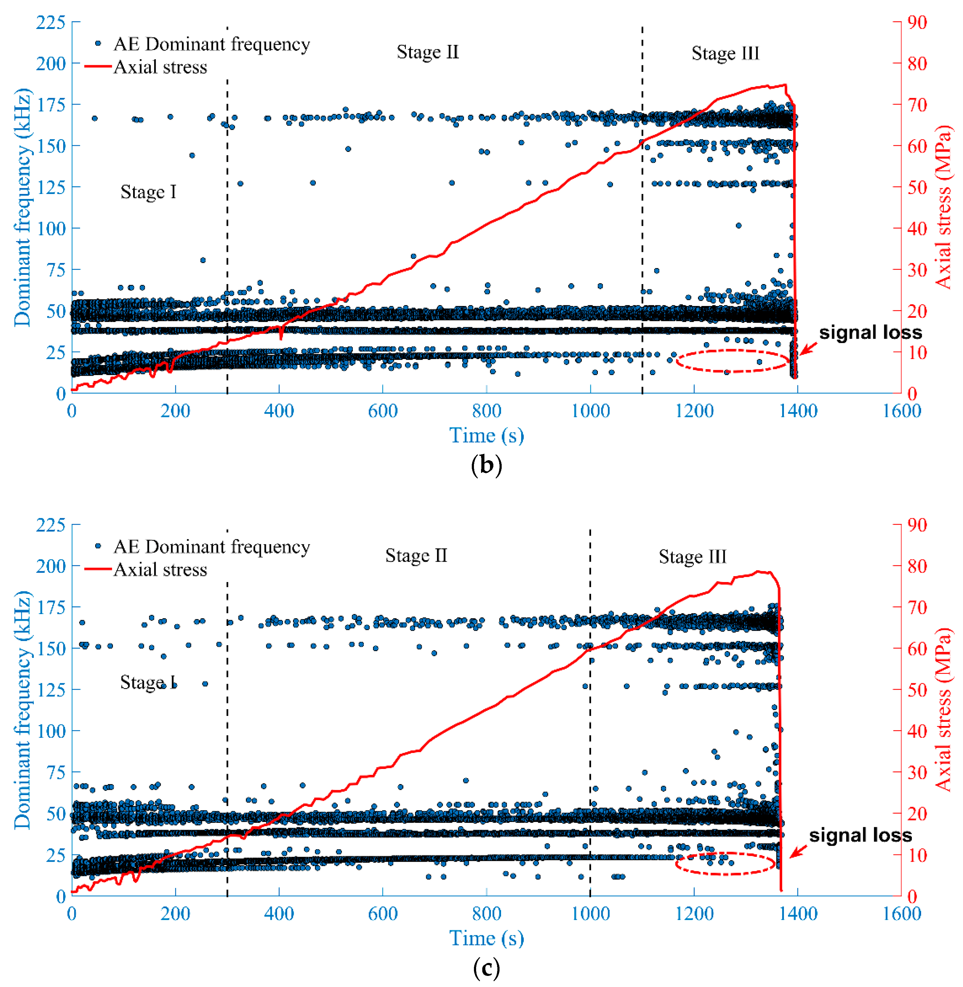
3. Analysis of the Dominant Frequency Characteristics of AE Signals

In this paper, due to space limitations, only the test results of X-1, X-3, and X-6 are considered as examples for detailed analysis. As shown in Figure 3, the loading process is divided into the following three stages: compaction to elastic deformation (stage I), microcrack stable development (stage II), and crack propagation to failure (stage III). During stage I, the pre-existent pore or microfissures in the specimen are gradually closed, and the rock is compacted to form early non-linear elastic deformation; during stage II, the process of compaction closure of the pre-existent pore or microfissures in the specimen ends, and the newly incubated microfissures develop steadily; during stage III, the development of microfissures changes qualitatively, and the fracture develops continuously until the end of the specimen, reaching total destruction. The main purpose of introducing three stages of the loading process is to demonstrate the dominant frequency evolution characteristics of AE in different deformation stages in detail, so as to strengthen the understanding of the rock fracture mechanism. The time–stress curve coupled with an AE signal can better reflect the failure evolution law of rock than the strain–stress curve [21]. Figure 3 shows the relationship between the dominant frequency and axial stress of each specimen in the entire test process with time.

It can be seen from Figure 3 that under a uniaxial compression condition, the fine sandstone exhibits clear distribution characteristics of double high and low dominant AE frequencies, both of which are below 200 kHz. The double dominant frequencies characteristics also exist in the AE test of marble [22]. For each specimen, according to the 0–10, 10–20, 20–30, …, 190–200 kHz frequency ranges, the dominant frequency of AE is evenly divided into 20 dominant frequency bands labeled from 1 to 20. The statistical results of the number of waveforms in different dominant frequency bands are shown in Figure 4 (the logarithmic coordinate axis is used in the longitudinal axis).

Figure 3 and Figure 4 indicate that the dominant frequency bands of fine sandstone were mainly distributed into high-frequency (120–180 kHz) and the low-frequency (10–70 kHz) bands, and the number of bands in the former is significantly less than that in the latter. He et al. [15] noted that different frequency components correspond to different fracture modes. Therefore, the AE signal in the low-frequency band of 30–70 kHz, which is always present in the entire test process, can be regarded as the inherent signal in the rock damage evolution process. In addition, Cai et al. [23] noted that the high-frequency AE signal corresponds to the initiation of microcracks, while the low frequency is associated with the formation of large cracks. It has been confirmed that AE frequency domain characteristics can reflect the crack size and type of rock fracture [5,24]. Based on referring to the existing research, in the present study, to describe the entire rock fracture process, the AE signal with a dominant frequency in the range of 120–180 kHz is regarded as the high-frequency signal corresponding to microcrack initiation, and that with a dominant frequency in the range of 10–30 kHz is regarded as the low-frequency signal corresponding to the large fracture formation.

In stage I, the primary pores and microcracks in the specimen were compacted and closed under load to lead to a certain degree of coalescence, thereby resulting in a large number of low-frequency signals. At this moment, new microcracks had not yet started to initiate, and thus, only a small number of high-frequency signals existed. After entering stage II, the compaction and closure process of the primary pores and microcracks gradually ended. The low-frequency signals gradually stabilized in the range of 20–22 kHz, with a significantly reduced number. Meanwhile, new microcracks started to be initiated in the specimen, and high-frequency signals appeared. As the load increased, the signals were clustered into distinct frequency bands, and the range of frequency bands became wider. As the load continued to increase, the specimen entered stage III, and the microcracks that had already been initiated inside the specimen began to change drastically. Therefore, the high-frequency signals, which were previously in the range of 165–170 kHz, had two new high frequency bands of 144–152 kHz and 125–129 kHz. It is worth noting that the low-frequency signals exhibited “signal loss” characteristics before the specimens were about to fail (see red dotted line in Figure 3). The reason is that a large number of new microcracks occur in the rock under high stress. These new cracks propagate, extend and form macrocracks with the cracks formed before. The propagation of AE signals is blocked by the macrocrack penetration process, which results in the “loss” of some signals. Shen et al. [25] believed that this phenomenon occurred because before the rock fractures, a large number of cracks are clustered inside; because of this clustering, the transient elastic waves of AE are severely attenuated, and some of these waves are even blocked by the cracks. This is consistent with the phenomena observed in the tests.

4. Analysis of AE Signal Amplitude and Fractal Characteristics

4.1. Characteristics of AE Signal Amplitude

The basic parameters of AE waveforms are generally represented by frequency and amplitude, and their dominant frequencies and corresponding amplitudes are important characteristic parameters that can reflect the scale and type of cracks during rock damage and fracture processes [24,26]. Figure 5 shows the three-dimensional (3D) time-frequency plot of the dominant frequency–amplitude–time for each specimen AE. The amplitudes and the occurrence times corresponding to the high and low dominant frequencies of the fine sandstone are intuitively observed.

Figure 5 shows that in the middle stage of loading in the test, the AE signals have small amplitudes, mostly below 10 mV (normalized amplitude < 0.1). In order to conveniently observe the amplitude distribution of the AE signal frequency corresponding to each specimen, normalization treatment is first carried out to transform the AE voltage amplitude into a dimensionless expression between [0, 1], which becomes a unified scalar, and subsequently, the main frequency versus amplitude diagram for all data points, in the order of low to high dominant frequencies, was plotted, as shown in Figure 6. It can be seen that both high-amplitude signals (normalized amplitude ≥ 0.1) and low-amplitude signals (normalized amplitude < 0.1) exist in the 10–70 kHz (low-frequency band) and 120–180 kHz (high-frequency band) double dominant frequencies of fine sandstone.

Therefore, in reference to Figure 5 and Figure 6, the AE signals in the frequency domain can be subdivided into four types of signals, i.e., low-frequency low-amplitude, low-frequency high-amplitude, high-frequency low-amplitude, and high-frequency high-amplitude signals. The analysis demonstrated that these four types of signals characterize the different sizes and types of cracks. In stage I, a large number of low-frequency high-amplitude signals and few high-frequency low-amplitude signals were generated. After the specimen entered stage II, the low-frequency high-amplitude signals decreased, and the signals consisted mainly of low-frequency low-amplitude and high-frequency low-amplitude signals. As stage III was reached, the low-frequency high-amplitude signals increased considerably. The amplitudes were extremely high, and the maximum values of the amplitudes since the beginning of loading occurred prior to rock fracture; in the meantime, a large number of high-frequency high-amplitude signals also appeared. A large number of low-frequency low-amplitude signals continued to appear during the entire specimen fracture process, indicating that this type of signal was caused by the movement and fracture of the internal lattice of the specimen. The high-frequency low-amplitude signals did not start to appear until stage II was reached; the number of these signals increased as the stress increased, and these signals corresponded to newly initiated microcracks. The high-frequency high-amplitude signals suddenly appeared before specimen fracture and corresponded to the closing of the already initiated microcracks to form small- and medium-scale cracks. The low-frequency high-amplitude signals appeared only in stages I and III; when the specimen fractured, the amplitude of the low-frequency signals was extremely high, higher than that of the signals in stage I, indicating that the low-frequency high-amplitude signals corresponded to the compaction of pores, the propagation and coalescence of small-scale cracks, and the formation of large-scale macrocracks.

4.2. Fractal Characteristics of AE Signal Amplitude

Fractal dimension is the most important concept in fractal theory and application. It is the most important index to measure the complexity of objects. For rock fracture, fractal dimension can reflect the intrinsic systematic evolution characteristics of rock. The increase and decrease of the fractal dimension indicate the decrease and increase of the orderly degree of crack development in rock failure [27]. The propagation and evolution process of internal microcracks during rock damage and fracture process has fractal characteristics, and the corresponding frequency-domain parameters of the AE waveforms can be viewed as a univariate time series set [28]. The GP algorithm can be used to calculate the relevant fractal dimension [18,27,29], which is one of the most commonly used fractal dimensions. The increase and decrease in the relevant fractal dimension indicate the decrease and increase, respectively, in the degree of order of the internal failure mode of a rock [21]. Using the peak strength as a baseline and assuming the stress ratio (percentage ratio of the axial stress to the peak intensity) to be 100%, the stress ratio of each specimen was divided into 10 stress ratio intervals (0–10%, 10–20%, and so on, up to 90–100%). However, even after the peak intensity was reached, the specimen could still bear the load for a certain period of time before complete failure occurred; this period of time was treated as a separate interval, resulting in a total interval of 11 intervals. The relevant fractal dimensions D1 and D2 of the amplitude of the AE signal in the 10–70 kHz (low-frequency) and 120–180 kHz (high-frequency) bands in different intervals were calculated for each specimen. Since there were fewer signals in the high-frequency band in the initial loading stage (stress ratio < 20%), only the signals in the high-frequency band after stress ratio ≥ 20% were considered for the calculation. The variation of relevant fractal dimension D with the stress ratio during the entire loading process in the test is shown in Figure 7.

Figure 7 indicates that D1 is generally lower than D2. In the early loading stage of the test, because the number and size of primary pores and microcracks inside the specimens varied, the compaction and closure process of the specimen often exhibited an evolution pattern from disorder to order. In a small range, D1 either first increased continuously and later decreased (X-1, X-3), or it first increased and later decreased in a fluctuating manner (X-6), corresponding to a process in which the primary pores and microcracks in the specimen were compacted and closed under loading, thereby generating a certain amount of coalescence. When the stress ratio was less than 50%, the pattern of D2 variation was not uniform. Some specimens (X-1 and X-3) exhibited a trend of first decreasing and later increasing, whereas one specimen (X-6) exhibited a trend of continuously increasing. Nevertheless, there was a growth process in both cases, indicating that the microcrack initiation process in the early loading stage of the test was propagated in a disordered manner with large randomness.

With the increase in the load, when the stress ratio reached approximately 50%, D1 started to rise continuously and gradually attained its peak value; this is because during stage II, the internal lattice of the specimen moved and fractured, and thus most of the released low-frequency signals had low and even amplitudes, which exhibited considerable dispersion and disorder. The stress ratio corresponding to the peak D1 was different for different specimens, indicating that the heterogeneity and anisotropy of the rock sometimes lead to large differences among different specimens [30]. Meanwhile, when the stress ratio was 50%, D2 exhibited a turning point as it started to continuously decrease from the peak, indicating that the microcrack initiation and development process of the specimen gradually stabilized and progressed in an orderly manner under moderate to high stresses in the middle and late loading stages.

As the load continued to increase, prior to specimen fracture, D1 exhibited a significant turning point with the occurrence of a sudden rapid drop; this is because in stage III, the signal amplitude of the low-frequency band began to exhibit a relatively high value, indicating the formation of large macrocracks. The signal amplitude of the high-frequency band also showed a relatively high value, and the development, propagation, and coalescence of microcracks led to the propagation and expansion of small- and medium-scale cracks approaching the macroscopic fracture surface, thereby causing D2 to decrease continuously.

5. Analysis of the Energy Ratio of Each AE Signal

5.1. Full Time-Domain Analysis

All AE waveforms of each specimen under the entire compression and fracture process were obtained and plotted according to the order of generation, as shown in Figure 8. The percentages of the number of AE waveforms of each specimen in different stress ratio intervals are provided in

Table 2. Statistics of AE waveform proportion in each loading stress ratio interval of specimens.

X-1			X-3			X-6
Stress Ratio (%)	Corresponding Time Period (s)	Waveform Proportion (%)	Stress Ratio (%)	Corresponding Time Period (s)	Waveform Proportion (%)	Stress Ration (%)	Corresponding Time Period (s)	Waveform Proportion (%)
[0, 10]	1~186	21.79	[0, 10]	1~177	19.86	[0, 10]	1~164	22.00
[10, 20]	187~394	15.53	[10, 20]	178~376	14.58	[10, 20]	165~350	12.15
[20, 30]	395~534	6.64	[20, 30]	377~513	6.74	[20, 30]	351~491	5.91
[30, 40]	535~667	5.03	[30, 40]	514~655	4.99	[30, 40]	492~630	4.41
[40, 50]	668~787	3.59	[40, 50]	656~754	3.14	[40, 50]	631~721	2.61
[50, 60]	788~906	2.78	[50, 60]	755~874	3.07	[50, 60]	722~830	2.49
[60, 70]	907~1030	2.79	[60, 70]	875~983	2.29	[60, 70]	831~953	2.51
[70, 80]	1031~1142	2.88	[70, 80]	984~1095	2.60	[70, 80]	954~1062	2.75
[80, 90]	1143~1260	5.28	[80, 90]	1096~1204	4.71	[80, 90]	1063~1158	4.28
[90, 100]	1261~1398	13.70	[90, 100]	1205~1377	29.24	[90, 100]	1159~1322	19.21
[100, Complete failure]	1399~1449	20.00	[100, Complete failure]	1378~1395	8.77	[100, Complete failure]	1323~1369	21.69

.

From Figure 8 and Table 2, it can be seen that the number of signals released by fine sandstone in the initial stage (stress ratio [0, 20]) and the end stage of the test (stress ratio [90, complete failure]) under uniaxial compression is much larger than that in the remaining intervals, i.e., the number of waveforms first decreased and later increased as the load increased. Additionally, most of the waveforms in the intervals of [0, 10] and [100, complete failure] had large amplitudes, especially those in the interval of [100, complete failure], in which a large number of continuous high-amplitude waveforms were released. It is worth noting that the maximum amplitude of the waveforms that were released during the entire process of each specimen often occurred when the specimen completely failed; further verifying that the high-amplitude signals corresponded to the macroscopic fracture of the specimen.

5.2. Wavelet Packet Band Decomposition

Wavelet packet analysis can decompose not only the low-frequency information of the signal but also the high-frequency information of the signal in real time, thereby improving the time-frequency resolution [31]. Wavelet packet decomposition was performed using the db3 wavelet as the wavelet base. According to the sampling law [32], the sampling frequency of the system was 1000 kHz, and the Nyquist frequency was 500 kHz. The signal was decomposed up to the fifth layer, and the frequency bandwidth corresponding to each node in the fifth layer was 15.625 kHz, totaling 32 frequency bands. After wavelet package decomposition, the frequency bands were rearranged to ensure the monotonic increase property of the frequencies.

5.3. Method to Calculate Wavelength Packet Reconstruction Signal Band Energy

When the AE signal was decomposed to the fifth layer, 32 component signals were generated. One of the analyzed signals was denoted as S_5,j(t), and its corresponding energy is E_5,j Thus [33]:

$$E_{5,j}=\int {\left|S_{5,j}\left(t\right)\right|}^{2}dt={\displaystyle \sum }_{k=1}^m{\left|x_{j,k}\right|}^2$$

(1)

where j = 0, 1, 2, …, 2⁵ − 1; m is the number of discrete sampling points of the signal; and x_j,k represents the magnitude of the discrete points in the signal S_5,j(t).

E₀ is the total energy of the analyzed signal, and can be written as:

$$E_0={\displaystyle \sum }_{j=0}^{2^5-1}{E}_{5,j}$$

(2)

P_j is the energy percentage of each sub-band of the analyzed signal, and can be written as:

$$P_j=\frac{E_{5,j}}{E_0}\times 100\%$$

(3)

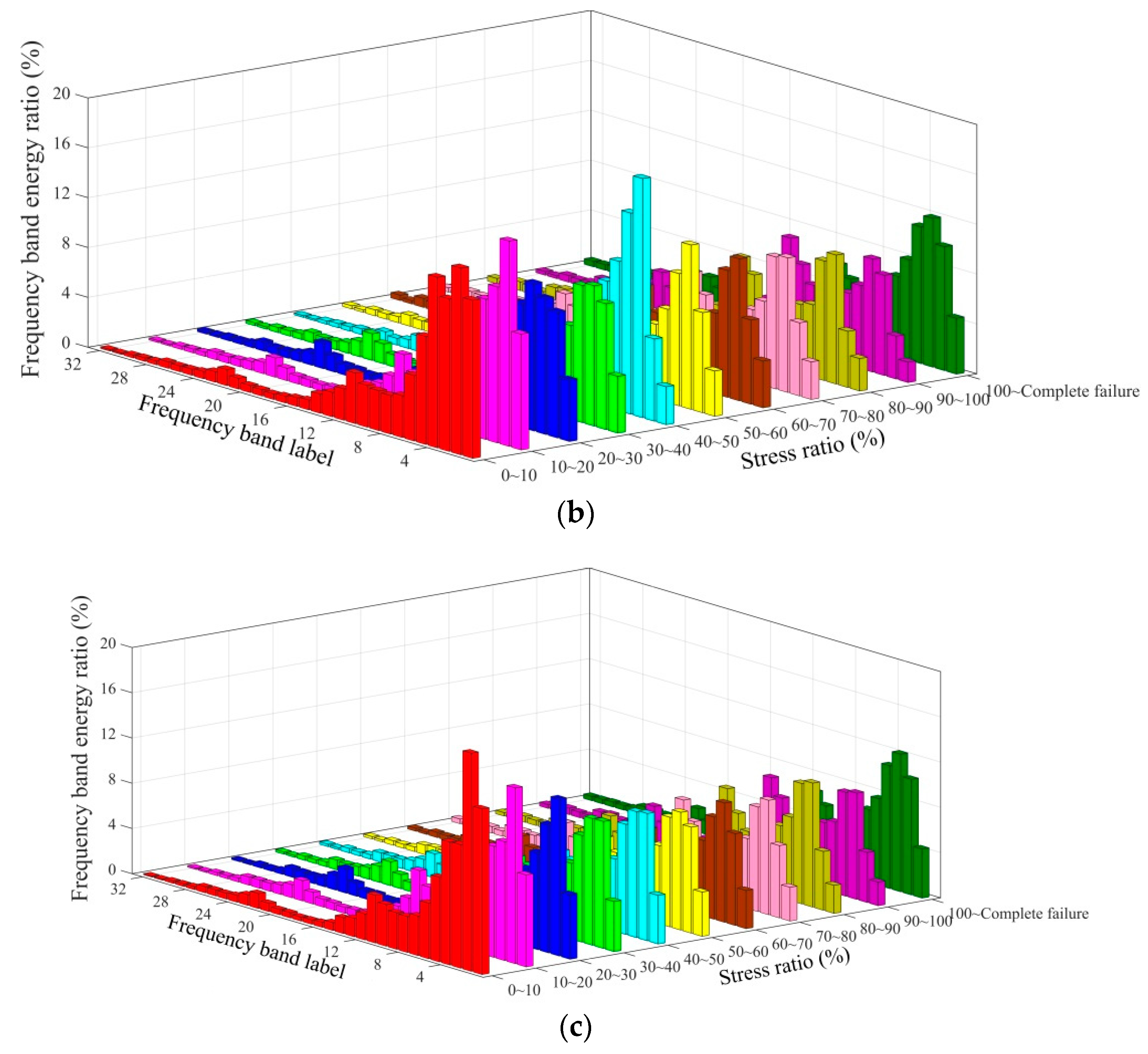
5.4. Energy Variation Pattern for AE Signal Bands

Based on Equations (1)–(3), the energy distribution of the frequency bands in different failure stages of the entire test process can be obtained. Figure 9 shows the 3D histogram of the band energy distribution for AE signals in each loading stress ratio interval during the entire test, and the frequency band labels are arranged in ascending order of the frequencies.

Figure 9 shows that the energy of the frequency band in the AE signal was concentrated mainly in bands 1 to 12, which had a sum of average energy ratios equal to 79%. However, within different stress ratio intervals, the energy ratio of each band did not exceed 20%. At the same time, it can be seen that as the load increased, the variation of the energy ratios of bands 1–3 and 10–12 were significant, especially those for bands 1, 2, 10, and 11. Figure 10 and Figure 11 show the relationship between the stress ratio and the average energy ratio of bands 1 and 2 in the low-frequency band and bands 10 and 11 in the high-frequency band, respectively.

From Figure 10 and Figure 11, a difference in the energy ratios of bands 1, 2, 10, and 11 of different specimens can be noted; however, their overall distribution patterns and changing trends were consistent. In the low-frequency bands, the energy ratios of bands 1 and 2 first decreased gradually with the increasing load, exhibiting the minimum value at a stress ratio of 90–100%, and later increased; further, the energy ratio of band 1 was always higher than that of band 2 in different failure stages. In the high-frequency bands, the energy ratios of bands 10 and 11 first increased gradually as the load increased, reaching the maximum value at a stress ratio of 90–100%, and later decreased; further, the energy ratio of band 10 was lower than that of band 11 in different failure stages. Therefore, after a specimen was subjected to compression, the compaction and closure of pores and microcracks inside the rock led to the concentration of band energy mainly in the low-frequency bands, with the energy ratios of bands 1 and 2 being high. As the load increased, the initiated microcracks developed steadily inside the rock, causing the energy ratios of bands 10 and band 11 in the high-frequency bands to increase continuously while causing the energy ratios of bands 1 and 2 in the low-frequency bands to decrease gradually. After the peak intensity was reached, the energy ratios of bands 1 and 2 increased, while those of bands 10 and 11 decreased, and all of these parameters demonstrated turning points because the microcracks clustering inside the rock became macroscopic large cracks, indicating the imminent complete failure of the rock. Therefore, it is further proven that the high-frequency band of the AE signal corresponds to the initiation of microcracks, and the low-frequency band corresponds to the formation of large cracks.

6. Conclusions

Based on the above analysis, the following conclusions can be drawn:

(1)

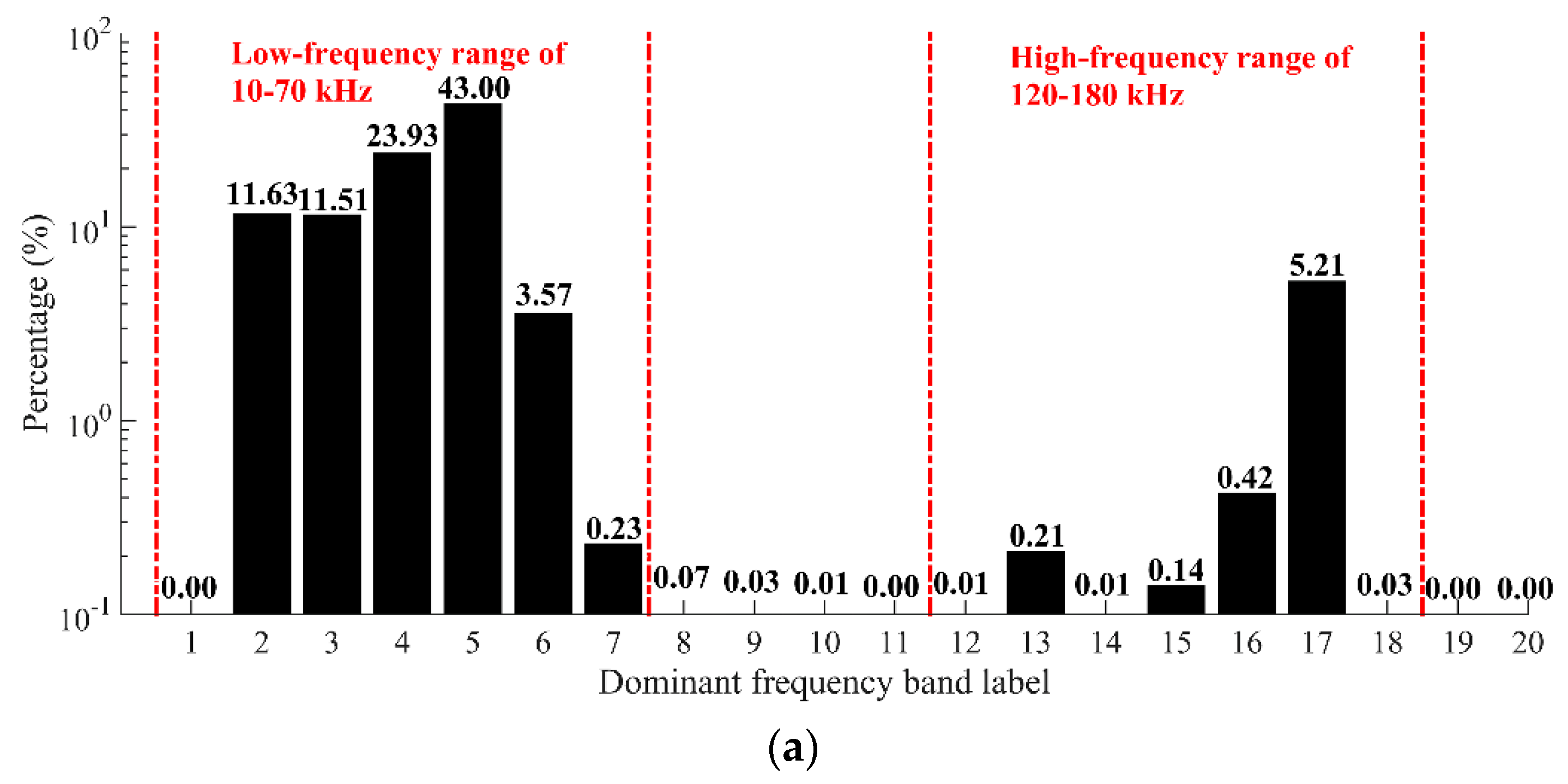
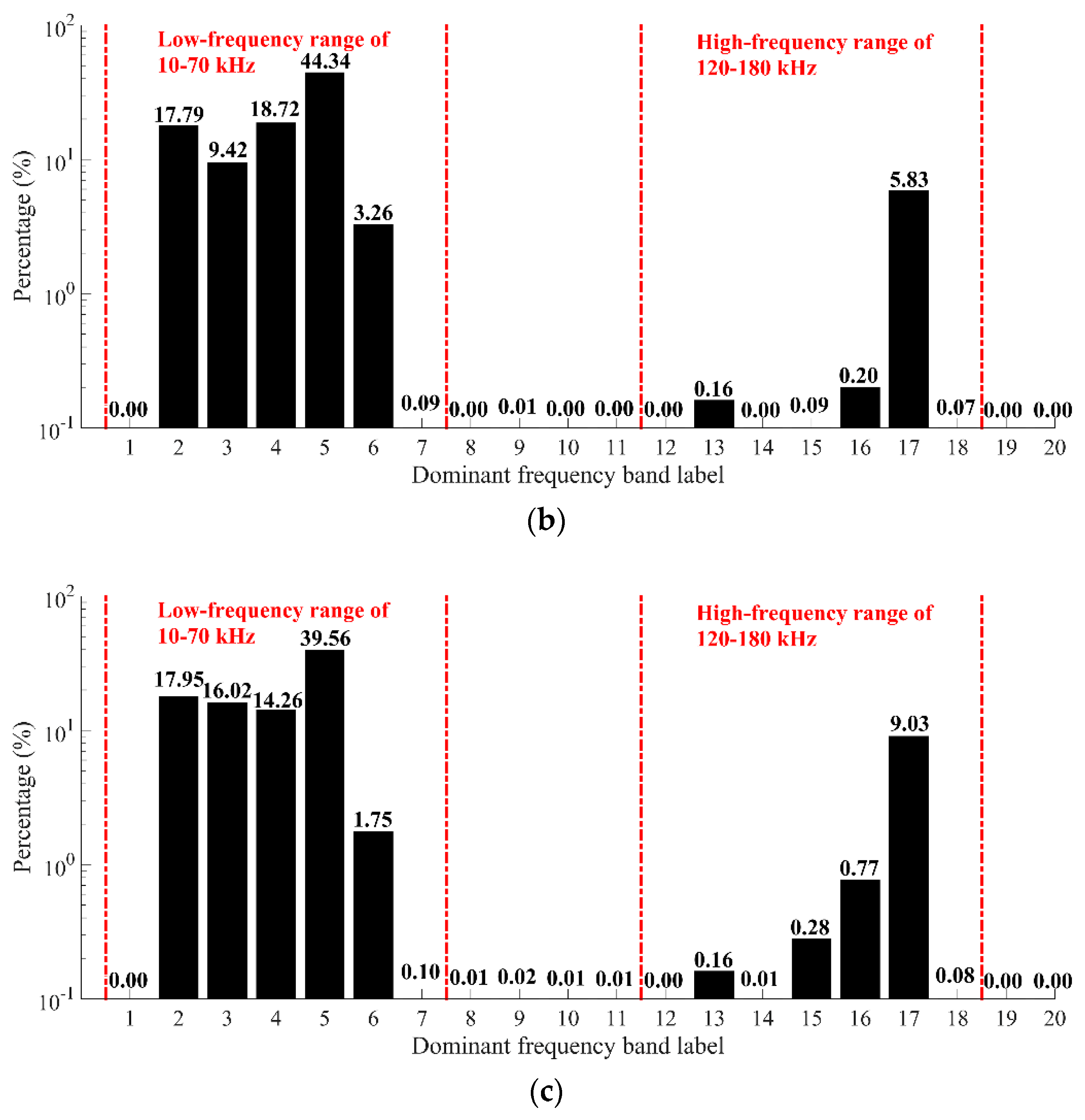
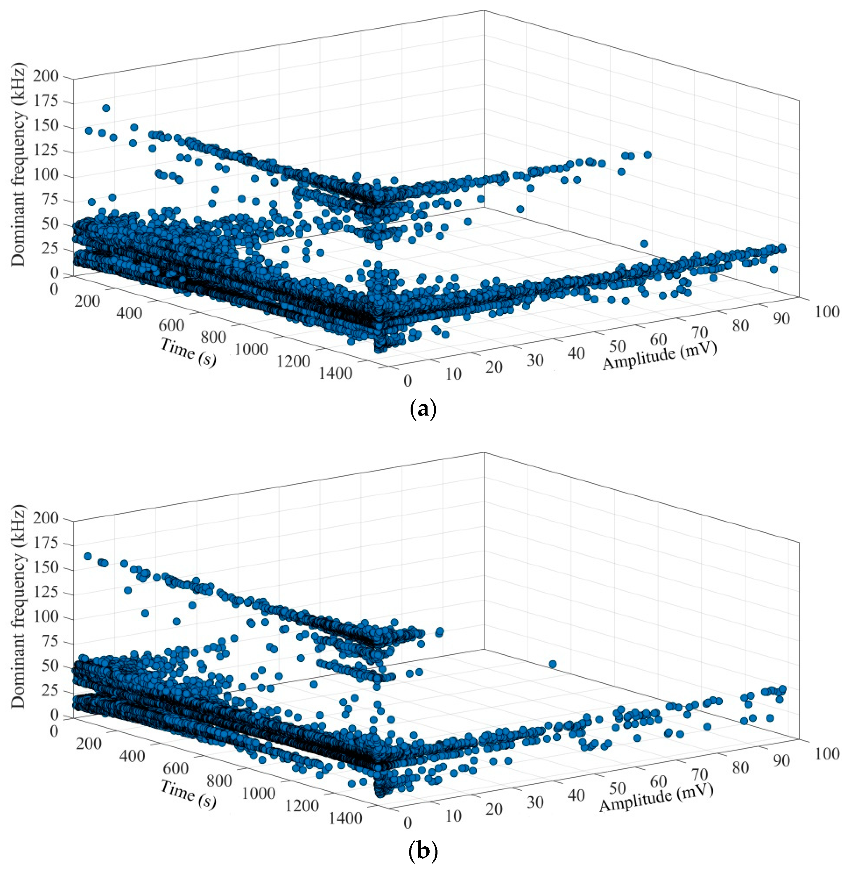
The AE signal during the entire fracture process of fine sandstone exhibited double dominant frequency bands. The low-frequency bands were concentrated at 10–70 kHz, the high-frequency bands were concentrated at 120–180 kHz, and the number of AE signals in the low-frequency bands was significantly higher than that in the high-frequency bands.

(2)

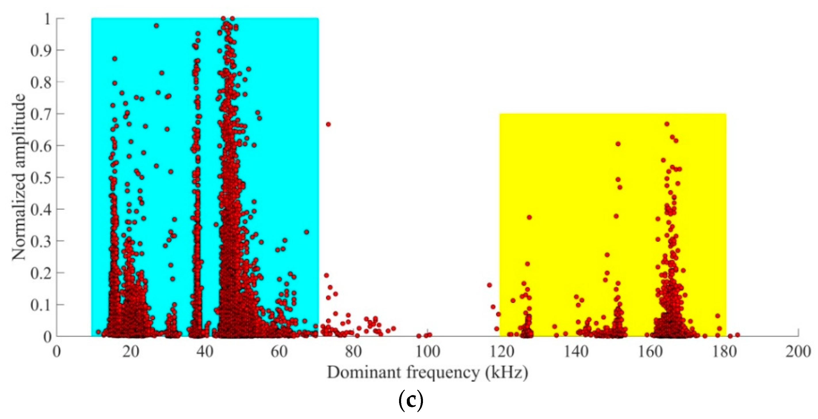
Combining the AE signal amplitude, the AE signals can be further subdivided into four types: low-frequency low-amplitude, low-frequency high-amplitude, high-frequency low-amplitude, and high-frequency high-amplitude signals. Different types of AE signals correspond to different types of fractures in rock.

(3)

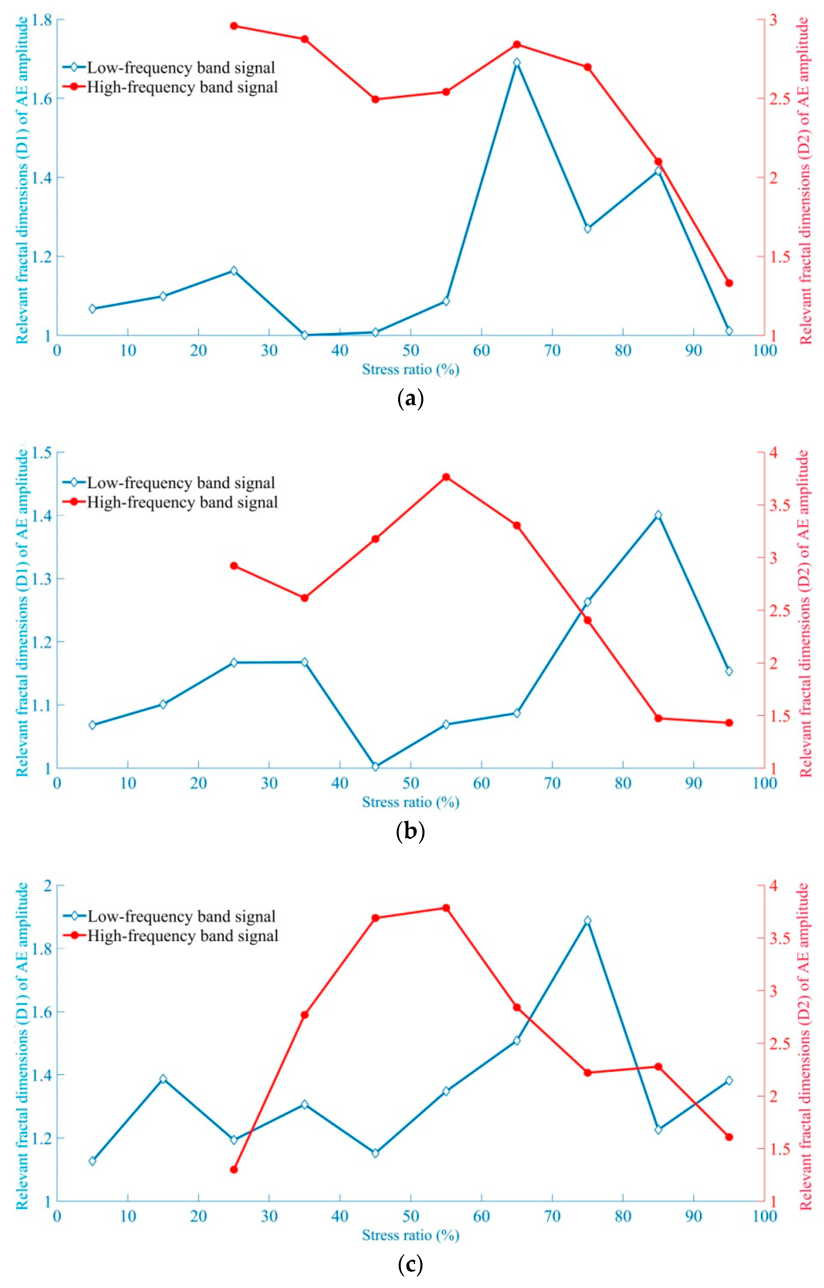
For AE signal amplitude, the relevant fractal dimension D1 of the low-frequency band was generally lower than the relevant fractal dimension D2 of the high frequency band. Both D1 and D2 had a significant turning point involving a decrease in magnitude. Before the stress ratio reached 50%, D1 fluctuated considerably; however, the trend can still be seen as one involving, first, an increase in the fractal dimension, and then a subsequent decrease. D2 increased in the early stage, and after the stress ratio reached 50%, D2 continued to decrease.

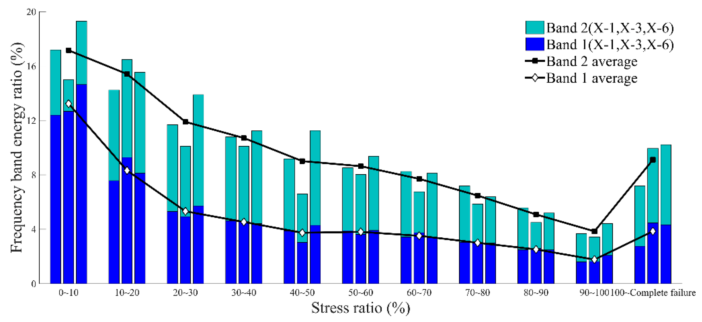
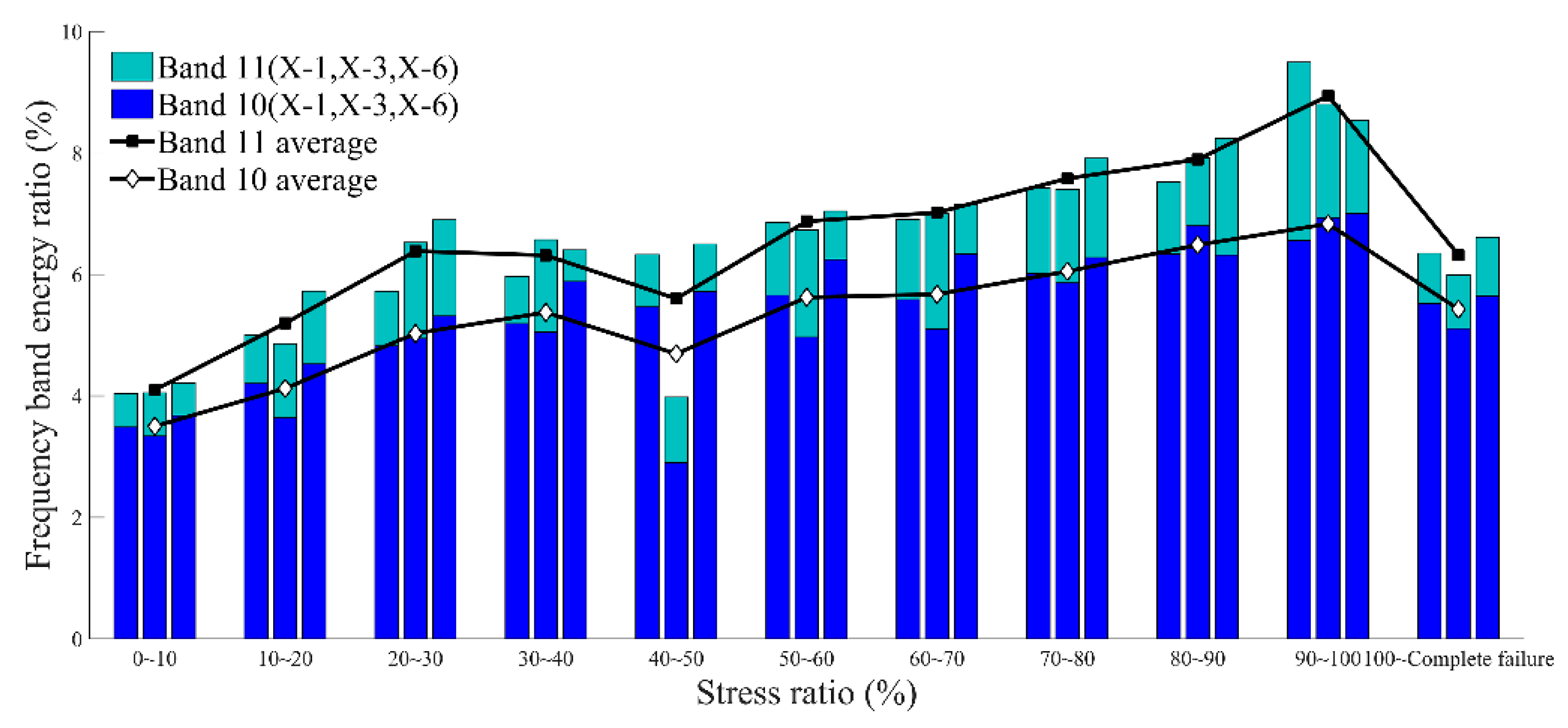
(4)

The band energy of the AE signal in the fine sandstone was concentrated mainly in the range of 0–187.5 kHz (bands 1–12) in different failure stages, and the sum of average energy ratios was up to 79%. However, even in different stress ratio intervals, the energy ratio of each band did not exceed 20%. The energy ratios of bands 1 and 2 in the low-frequency band as well as those of bands 10 and 11 in the high-frequency band varied significantly with the stress ratio. Bands 1 and 2 exhibited the trend of first decreasing and later increasing, exhibiting the minimum value at a stress ratio of 90–100%; bands 10 and 11 exhibited the trend of first increasing and later decreasing, exhibiting the maximum value at a stress ratio of 90–100%.

References

1. Scruby, B.C. An introduction to acoustic emission. J. Phys. E. 1987, 20, 946–953. [Google Scholar] [CrossRef]
2. Ji, H.G. Research and Application on Acoustic Emission Performance of Concrete Material; China Coal Industry Publishing House: Beijing, China, 2004; pp. 1–2. [Google Scholar]
3. Lavrov, A. The Kaiser effect in rocks: Principles and stress estimation techniques. Int. J. Rock Mech. Min. 2003, 40, 151–171. [Google Scholar] [CrossRef]
4. Liu, J.P.; Li, Y.H.; Xu, S.D.; Xu, S.; Jin, C.Y.; Liu, Z.S. Moment tensor analysis of acoustic emission for cracking mechanisms in rock with a pre-cut circular hole under uniaxial compression. Eng. Fract. Mech. 2015, 135, 206–218. [Google Scholar] [CrossRef]
5. Li, L.R.; Deng, J.H.; Zheng, L.; Liu, J.F. Dominant frequency characteristics of acoustic emissions in white marble during direct tensile tests. Rock Mech. Rock Eng. 2017, 50, 1337–1346. [Google Scholar] [CrossRef]
6. Sondergeld, C.H.; Estey, L.H. Acoustic emission study of microfracturing during the cyclic loading of Westerly granite. J. Geophys. Res. 1981, 86, 2915–2924. [Google Scholar] [CrossRef]
7. Cai, M.; Morioka, H.; Kaiser, P.K.; Tasaka, Y.; Kurose, H.; Minami, M.; Maejima, T. Back-analysis of rock mass strength parameters using AE monitoring data. Int. J. Rock Mech. Min. 2007, 44, 538–549. [Google Scholar] [CrossRef]
8. Du, F.; Wang, K.; Wang, G.D.; Jiang, Y.F.; Xin, C.P.; Zhang, X. Investigation on acoustic emission characteristics during deformation and failure of gas-bearing coal-rock combined bodies. J. Loss Prev. Process Ind. 2018, 55, 253–266. [Google Scholar] [CrossRef]
9. Farahat, A.M.; Ohtsu, M. Evaluation of plastic damage in concrete by acoustic emission. J. Mater. Civ. Eng. 1995, 7, 148–153. [Google Scholar] [CrossRef]
10. Bagde, M.N.; Petros, V. Fatigue and dynamic energy behaviour of rock subjected to cyclical loading. Int. J. Rock Mech. Min. 2009, 46, 200–209. [Google Scholar] [CrossRef]
11. Moradian, Z.; Einstein, H.H.; Ballivy, G. Detection of cracking levels in brittle rocks by parametric analysis of the acoustic emission signals. Rock Mech. Rock Eng. 2016, 49, 785–800. [Google Scholar] [CrossRef]
12. Shiotani, T.; Ohtsu, M.; Ikeda, K. Detection and evaluation of AE waves due to rock deformation. Constr. Build. Mater. 2001, 15, 235–246. [Google Scholar] [CrossRef]
13. Stefano, D.S.; Adrienn, K.T. Laboratory and field studies on the use of acoustic emission for masonry bridges. NDT E Int. 2013, 55, 64–74. [Google Scholar]
14. Aker, E.; Kuhn, D.; Vavrycuk, V.; Soldal, M.; Oye, V. Experimental investigation of acoustic emissions and their moment tensors in rock during failure. Int. J. Rock Mech. Min. 2014, 70, 286–295. [Google Scholar] [CrossRef]
15. He, M.C.; Zhao, F.; Zhang, Y.; Du, S.; Guan, L. Feature evolution of dominant frequency components in acoustic emissions of instantaneous strain-type granitic rockburst simulation tests. Rock Soil Mech. 2015, 36, 1–8. [Google Scholar]
16. Ji, H.G.; Wang, H.W.; Cao, S.Z.; Hou, Z.F.; Jin, Y. Experimental research on frequency characteristics of acoustic emission signals under uniaxial compression of granite. Chin. J. Rock Mech. Eng. 2012, 31, 2900–2905. [Google Scholar]
17. Morgan, S.P.; Johnson, C.A.; Einstein, H.H. Cracking processes in Barre granite: Fracture process zones and crack coalescence. Int. J. Fract. 2013, 180, 177–204. [Google Scholar] [CrossRef]
18. Zhao, K.; Wang, G.F.; Wang, X.J.; Jin, J.F.; Deng, F. Research on energy distributions and fractal characteristics of Kaiser signal of acoustic emission in rock. Rock Soil Mech. 2008, 29, 3082–3088. [Google Scholar]
19. Lai, Y.S.; Xiong, Y.; Cheng, L.F. Frequency band energy characteristics of acoustic emission signals in damage process of concrete under uniaxial compression. J. Vib. Shock 2014, 11, 177–182. [Google Scholar]
20. Chen, S.W.; Yang, C.H.; Wang, G.B.; Liu, W. Similarity assessment of acoustic emission signals and its application in source localization. Ultrasonics 2017, 75, 36–45. [Google Scholar] [CrossRef]
21. Cong, Y.; Feng, X.T.; Zheng, Y.R.; Wang, Z.Q.; Zhang, L.M. Experimental study on acoustic emission failure precursors of marble under different stress paths. Chin. J. Geotech. Eng. 2016, 38, 1193–1201. [Google Scholar]
22. Deng, J.H.; Li, L.R.; Chen, F.; Liu, J.F.; Yu, J. Twin-peak Frequencies of Acoustic Emission Due to the Fracture of Marble and Their Possible Mechanism. Adv. Eng. Sci. 2018, 50, 12–17. [Google Scholar]
23. Cai, M.; Kaiser, P.K.; Morioka, H.; Minami, M.; Maejima, T.; Tasaka, Y.; Kurose, H. FLAC/PFC coupled numerical simulation of AE in large-scale underground excavations. Int. J. Rock Mech. Min. 2007, 44, 550–564. [Google Scholar] [CrossRef]
24. Zhu, Z.F.; Chen, G.Q.; Xiao, H.Y.; Liu, H.; Zhao, C. Study on crack propagation of rock bridge based on multi parameters analysis of acoustic emission. Chin. J. Rock Mech. Eng. 2018, 37, 909–918. [Google Scholar]
25. Shen, B.T.; Stephansson, O.; Rinne, M. Modelling of Rock Fracturing Processes; CSIRO Earth Science and Resource Engineering: Brisbane, QLD, Australia, 2014; pp. 5–18. [Google Scholar]
26. Zeng, P.; Liu, Y.J.; Ji, H.G.; Li, C.J. Coupling criteria and precursor identification characteristics of multi-band acoustic emission of gritstone fracture under uniaxial compression. Chin. J. Geotech. Eng. 2017, 39, 509–517. [Google Scholar]
27. Chen, M.; Yang, S.Q.; Pathegama, G.R.; Yang, W.D.; Yin, P.F.; Zhang, Y.C.; Zhang, Q.Y. Fracture processes of rock-Like specimens containing nonpersistent fissures under uniaxial compression. Energies 2019, 12, 79. [Google Scholar] [CrossRef]
28. Zhang, Z.B.; Wang, E.Y.; Li, N. Fractal characteristics of acoustic emission events based on single-link cluster method during uniaxial loading of rock. Chaos Solitons Fract. 2017, 104, 298–306. [Google Scholar] [CrossRef]
29. Grassberger, P.; Procaccia, I. Characterization of strange attractors. Phys. Rev. Lett. 1983, 50, 346–349. [Google Scholar] [CrossRef]
30. Wu, X.Z.; Liu, X.X.; Liang, Z.Z.; Liu, X.; Yu, M. Experimental study of fractal dimension of acoustic emission serials different of different rocks under uniaxial compression. Rock Soil Mech. 2012, 33, 3561–3569. [Google Scholar]
31. Ling, T.H.; Liao, Y.C.; Zhang, S. Application of wavelet packet method in frequency band energy distribution of rock acoustic emission signals under impact loading. J. Vib. Shock 2010, 10, 127–130. [Google Scholar]
32. Chaparro, L. Signals and Systems Using MATLAB, 2nd ed.; Academic Press: Pittsburgh, PA, USA, 2015; pp. 333–396. [Google Scholar]
33. Stormy, A. MATLAB: A Practical Introduction to Programming and Problem Solving, 4th ed.; Butterworth-Heinemann Elsevier Ltd.: Oxford, UK, 2017; pp. 443–501. [Google Scholar]
Figure 1. The test system. (a) Uniaxial testing machine; (b) Extensometer; (c) Acoustic emission (AE) monitoring system.
Energies 12 03959 g001
Figure 2. Axial stress–strain curves of specimens.
Energies 12 03959 g002
Figure 3. Relationship curves of time with AE dominant frequency and axial stress in the entire test process. (a) X-1 specimen; (b) X-3 specimen; and (c) X-6 specimen.
Energies 12 03959 g003aEnergies 12 03959 g003b
Figure 4. Dominant frequency characteristics of specimens. (a) X-1 specimen; (b) X-3 specimen; (c) X-6 specimen.
Energies 12 03959 g004aEnergies 12 03959 g004b
Figure 5. The 3D time-frequency plot of the dominant frequency–amplitude–time of specimens. (a) X-1 specimen; (b) X-3 specimen; (c) X-6 specimen.
Energies 12 03959 g005aEnergies 12 03959 g005b
Figure 6. Normalized main frequency amplitude and count rate of specimens. (a) X-1 specimen; (b) X-3 specimen; and (c) X-6 specimen.
Energies 12 03959 g006aEnergies 12 03959 g006b
Figure 7. Variation of relevant fractal dimensions of AE amplitude with stress ratio in low- and high-frequency bands. (a) X-1 specimen; (b) X-3 specimen; (c) X-6 specimen.
Energies 12 03959 g007
Figure 8. AE waveforms of specimens during the entire test. (a) X-1 specimen; (b) X-3 specimen; and (c) X-6 specimen.
Energies 12 03959 g008aEnergies 12 03959 g008b
Figure 9. The 3D histogram of the band energy distribution for AE signals in each loading stress ratio interval during the entire test. (a) X-1 specimen; (b) X-3 specimen; (c) X-6 specimen.
Energies 12 03959 g009aEnergies 12 03959 g009b
Figure 10. The relationship between the stress ratio and the average energy ratio in the low-frequency band (bands 1 and 2).
Energies 12 03959 g010
Figure 11. The relationship between the stress ratio and the average energy ratio in the high-frequency band (bands 10 and 11).
Energies 12 03959 g011