1. Introduction
Over the last few decades, the environmental issues have increased at an alarming rate leading to governmental actions and policies towards the protection of the environment. The German Federal Government has set demanding goals related to the reduction of greenhouse gas (GHG) emissions with the German Climate Action Plan 2050 (Klimaschutzplan 2050) which is an implementation of the Paris Agreement. Aiming at decreasing GHG emissions by 2050 to 20% compared to the level of 1990, substantial measures must be taken in every emission producing sector to achieve this objective [
1]. Examples of sectors with GHG emissions are energy industries, manufacturing industries and construction, transport and households.
Focusing on transport, conventional cars are responsible for around 11% of the total CO
2 emissions in Germany. Besides its contribution to global warming, road transportation is responsible for 30% of NO
X and 12% of particulate matter emissions, which have shown to have a significant impact on human life expectancy [
2]. Electric vehicles (EVs) are an emerging clean technology, with battery EVs generating zero direct CO
2 emissions in the atmosphere. So far, EVs have been in the center of most strategies to mitigate GHG emissions and reach the set climate targets. Since EVs create no tailpipe emissions, these hazardous pollutants can be reduced, especially in urban areas. Supported by incentive programs, the number of EVs has risen to three million units in 2017, an increase of 50% in comparison to 2016 [
3]. According to the Global EV Outlook [
3], the number of EVs worldwide could exceed 130 million by 2030 under the assumption that government policies continue supporting the expansion of electromobility.
However, the expected growing number of EVs does not only offer advantages. EVs have high loads especially with their increasing battery capacities and charging rates. Since drivers tend to change in times when electrical grids are already highly loaded, for example after going back home from work, EVs can cause considerable congestion in electrical networks [
4,
5], especially in residential areas. EV charging load when uncontrolled may be added to pre-existing peak load overloading grid components such us transformers or causing poor power quality [
6]. The EV high penetration in the next years can have even worse consequences for the electric grid, posing significant challenges for distribution system operators.
One way to mitigate these consequences is charging scheduling strategies or grid services (voltage regulation, frequency regulation, reserves, etc.) from parked idle EVs [
7,
8]. Both charging strategies and grid services support high introduction of EVs, decrease electrical grid impact, and allow higher penetration of renewable generation. Different charging scheduling schemes can be devised based on different objectives either related to costs or to renewable energy consumption or other.
This paper contributes to the state of the art by providing a comprehensive impact study of uncoordinated, as well as coordinated, EV charging on a European semi-urban low voltage grid considering the effects on voltage stability, load flow, and phase unbalances. We model the low voltage grid as a three-phase system and use a validated stochastic availability model for EVs based on statistical data to simulate the impact of EV charging. Subsequently, we show the impact of uncoordinated charging and develop optimal charging strategies based on different objectives, including strategies to achieve low energy cost and to reduce GHG emissions. Finally, we analyze different output parameters of our low voltage grid model in detail.
This work is structured as follows. In
Section 2, related work is reviewed. The methodological approach of this work is presented in
Section 3, which includes the automated generation of the simulation model. In
Section 4, the results are discussed.
Section 5 gives a conclusion and an outlook on future work.
2. Related Work
This section describes previous studies that focus on modeling of low voltage grids, as well as charging strategies, for the optimized integration of EVs into the grid.
2.1. Modeling of Low Voltage Grids
An essential part of an EV impact study on the electrical grid is the distribution grid modeling. The grid models used and the depth of the grid simulations vary greatly throughout literature. Many previous studies, such as [
5,
9,
10], model the grid as a perfectly balanced three phase system. These approaches often omit the voltage unbalances which occur between the power lines in real-world systems resulting in lack of representativeness. Additionally, the most commonly used grid models (e.g., [
11]) are test feeders provided by the Institute of Electrical and Electronics Engineers (IEEE) [
12], which were originally designed to stress load flow algorithms [
12,
13]. These models are less suitable for EV impact studies as the overall design and data available were published for specific issues [
14].
On the other hand, there are some publications which use model-based real grids [
15,
16,
17]. These grids can be used to study the impact of low carbon technologies on a specific area or neighborhood, however this approach limits the representative character of the case studies. The size of the network should be considered in order to have reliable results because small-scale networks miss heterogeneity [
14]. Hence, in this study, we focus on a semi-urban low voltage grid which serves as a representative grid in Europe.
2.2. Charging Strategies
A substantial number of contributions address the optimized charging of EVs with different objectives, e.g., cost-minimizing. Linear Programming is commonly found to tackle optimization problems. For instance, in the Edison Project [
18], linear programming is utilized to charge EVs as cost-efficient as possible. In [
18], Aabrandt et al. discussed the mathematical models for EV aggregators in detail. In Jin et al. [
19], a linear program was formulated to maximize profits of aggregators. Lui et al. [
20] present a chance-constrained mixed-integer programming solution for aggregator based scheduling of EVs. Grid constraints are included with the help of flexible energy pricing. The overall objective is the minimization of the cost of energy. In Jin et al. [
21], the authors applied mixed-integer linear programming to schedule EV charging from an electricity market perspective with consideration for energy trading in real-time and in the day-ahead market. The objective in [
21] is revenue maximization of the aggregators. Distributed offline and online algorithms are proposed in Mukherjee and Gupta [
22] to schedule EVs in a multi aggregator market. The authors formulate a bi-objective optimization problem to maximize both the profit of the aggregators, as well as the total number of EVs charged. Besides linear optimization, Hutterer et al. [
23] employ evolutionary computation in a multi-agent distributed algorithm. The evolutionary computation enables the EVs energy demand, as well as the criterion of secure power grid operation, to be satisfied, under consideration of uncertainties. A similar optimization approach is taken by Lee et al. [
24]. The work aims at minimizing the load at a charging station with genetic optimization and was able to reduce the peak load of a charging task by up to 4.9%. In Yang et al. [
25] quadratic programming is used in a centralized framework to schedule EVs so that they are charged with electricity provided by wind power.
To sum up, there is a lot of literature available for the modeling of low voltage grids and optimized charging strategies. Nevertheless, we identified some research gaps, as a lot of papers, like ([
19,
22,
24]), omit the grid as a limiting factor when it comes to the charging of EVs. Our paper has the following main goals:
Model a realistic and representative semi-urban low voltage grid in a simulation environment.
Evaluate the impact of uncoordinated charging on low voltage networks realistically and as representatively as possible using criteria such as voltage drop, voltage unbalance, and thermal rating of cables used in the grid.
Use the representative grid model to test and asses different optimized strategies, based on different objectives, such as cost reduction or grid-friendliness.
3. Methodology
To evaluate the grid impact of uncoordinated charging (UC) and different optimized charging strategies, called coordinated charging (CC), we model a representative low voltage grid. In this context, we define UC as the process where EV users arrive home, plug in their vehicle, the charging process starts immediately, and the vehicle charges until it is full or used again. EV buyers and users are predominately middle-aged people in a technical profession, with high socioeconomic status, who are living in a suburban or rural multi-person household with high-income [
26]. Therefore, we have chosen grid #13, a semi-urban European low voltage grid published by the Distribution System Operator Observatory (DSOO) [
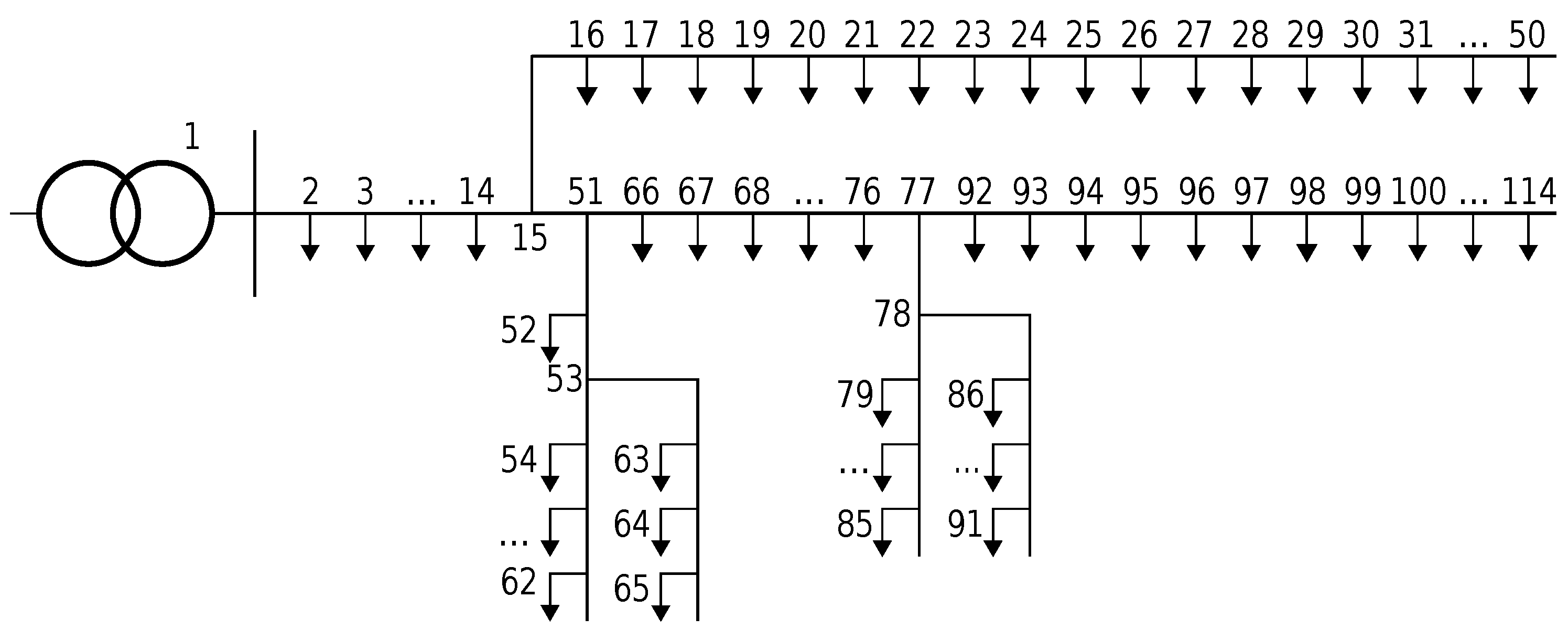
12].
Figure 1 depicts the single line diagram of the network, which consists of one transformer, 115 buses and 108 consumers at the 230
level. As we aimed at studying different scenarios, regarding the penetration rates of EVs and photovoltaics (PVs) installations, the development of the grid model was automated in MATLAB Simulink.
3.1. Modeling Framework
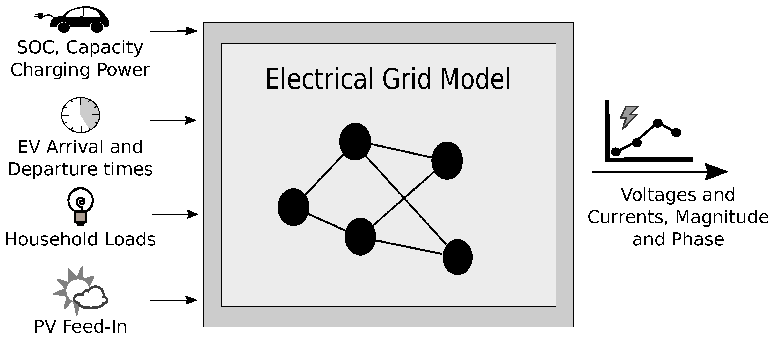
Figure 2 shows our conceptual approach with input and output data of our grid model. The EV data like the capacity of the battery or the maximum charging rate is based on the manufactures specifics. The investigated fleet is based proportionally on the EV sales in Germany since 2010 [
27]. The state of charge (SOC) of the EVs is calculated according to the energy consumption rate (ECR) measured by the German Automotive Club [
28] which includes also heating, ventilation and air conditioning (HVAC). The availability of EVs is based on arrival and departure times. In general, every EV can have more than one departure and arrival time per day based on statistical data. The detailed modeling approach of arrival and departure times can be found in Schlund et al. [
29]. Since data of EV usage, in general, is sparse, usage profiles are based on a survey of conventional traffic conducted by the German federal ministry of transportation. The availability mode of EVs is validated together with domain experts. Furthermore, the coincidence factors for different charging power levels of our model are in perfect agreement with figures found in literature [
30].
To model household loads, we work with synthesized load profiles generated with the load profile generator [
31]. As we are modeling a semi-urban low voltage grid, we assume all consumers to be either single-family homes or a mixture between single-family homes and duplex homes based on the evaluated scenario. We define two load cases; the heavy load case consists of 78 single-family homes and 30 duplex homes placed randomly into the grid, while the light load case is composed of 108 single-family homes. We incorporate PV systems in our model because other studies found a high affinity for renewable energy among EV users [
32]. The PV feed-in data is generated using the Photovoltaic Geographical Infractions System [
33], with Erlangen (Germany) as the selected location. Electricity prices and electricity generation are taken from the SMARD database [
34]. All data has a resolution of 15 min. For our simulation, we choose one summer and one winter week to study the seasonal difference regarding the impact of EV charging on the electric grid model.
3.2. Electrical Grid Model
The semi-urban low voltage grid is modeled as a three-phase system in the Simpscape Electrical environment of MATLAB. The model runs as a quasi-steady model; therefore, transient states are omitted, while it is still operating in a time-domain environment. The automated creation of our network is based on a script provided by Mathworks [
35]. The model is built with ideally grounded bus bars, as recommend by Olivier et al. [
36]. We omit the capacitance between lines and between line and earth because distribution networks are relatively small and therefore, the overall capacitance can be neglected (c.f. [
37,
38]). At every bus bar and in every line of the network we measure magnitude and phase of voltage and current. The simulation method allows us to capture phenomena at a selected frequency; we conduct our studies at the nominal frequency for Europe, 50 Hz. The automated development of our model is able to distribute a selected quantity of PV installations, as well as EVs, throughout the electrical network. Furthermore, the phase connection of load and the distribution of loads throughout the network can be varied.
3.3. Charging Strategies
We assume that the charging of the EV in the residential setting is only limited by the maximum charging rate of the vehicle. The time frame in which a vehicle is able to charge is set by its arrival time and the next departure time. We study a number of different charging strategies, as there are different participants in the electrical charging process with different interests:
End consumers, who want to charge as much self-produced electricity as possible. Additionally, they possibly want to minimize the GHG emissions of the energy mix which is used for charging EVs.
Distribution system operators, who have to ensure safe operating conditions and want to minimize network losses.
Aggregators, who want to maximize their profits by obtaining energy as cheaply as possible.
We assume perfect foresight for all our charging strategies, meaning within our optimization horizon of one week all the arrival and departure times of our vehicles are known beforehand. Therefore, we also know the state of charge of the vehicles when they arrive at home. The parameters and functions used in the optimizations are as follows.
Sets and indexes:
| : | Number of vehicles |
| : | Number of discrete time steps |
| : | Number of PV installations |
| N | : | Set of vehicles |
| T | : | Set of time steps |
| : | Set of PV installations |
| : | Time step length (e.g., h) |
| n | : | Vehicle index |
| t | : | Time step index |
| o | : | PV installation index |
| : | Number of departures/arrivals of vehicle |
| : | Set of arrival times of vehicle : |
| : | Set of departure times of vehicle : |
Optimization variable:
| : | Charging power of n-th vehicle at time step |
Parameters and functions:
| | | |
| : | Electricity price at time step |
| : | Baseload function of aggregated household baseloads at time step |
| : | PV feed-in of PV-installation at time step |
| : | Battery capacity of vehicle |
| : | GHG emissions at time step |
| : | Charging power rate of vehicle |
| : | Transformer apparent power limit/cap |
| : | j-th arrival time of vehicle |
| : | j-th departure time of vehicle |
| : | State-of-Charge at arrival time |
| : | Mean of the sum of the baseload and all charging powers over all time steps |
3.3.1. Cost Optimized Strategy
This strategy revolves around the aggregator’s interest to maximize profits. Therefore, charging scheduling aims to minimize the energy cost for charging, as well as satisfying EV users requirements. Depending on the regulatory framework, electrical grid constraints have to be considered.
Equation (1) is the linear price objective function in which the sum of all charging demands of all vehicles at a time step is multiplied by the energy cost at the time step and the length of the time step. Subsequently, the result is summed up over all time steps. Equation (1b) ensures that every vehicle is charged fully between the time period of arrival and departure. For every vehicle, the charged energy equals the difference between 1 and the state of charge at arrival multiplied by the capacity of the vehicles’ battery. Equation (1c) forces the optimization variables to be zero if the vehicle is not at home. Due to grid constraints, we introduce a transformer limit which limits the sum of the baseload and the aggregated EV charging demand of all vehicles in a given time step (c.f. Equation (1d)). Equation (1e) assures, that the variable charging power does not exceed the maximum charging rate. Lastly, Equation (1f) ensures that the charging demand can be not-negative meaning the vehicles are not allowed feed back into the grid. Please note, this optimization strategy could also be applied to the end consumer if a tariff with spot price dependent energy prices is provided by an energy supply company.
3.3.2. Valley Filling (VF) Optimized Strategy
The objective of this strategy is to avoid congestion at peak times and shift load between 10 p.m. and 6 a.m. (load shifting method), achieving steady and low utilization of electrical equipment. With its focus on electrical grid constraints and low network losses, this scheduling process relies on network data, load information, and EV user data. The minimization of network losses is of great economic importance to the DSO because, with lower network losses, the margin of profit is increasing. Since this strategy does not consider any other objectives, the accumulated charging cost can be higher. VF can be achieved by minimizing the variance of the aggregated load at the transformer.
Equation (2a) is the summed up variance over the optimization time horizon. Further constraints (Equation (2b–2e)) of this strategy are already explained above. Please note, as a minimization of variance tries to keep the overall values as close as possible to the mean and therefore penalizing high aggregated load at the transformer, there is no need for an apparent transformer limit.
3.3.3. GHG Emission Optimized Strategy
This approach aims to be as climate-friendly as possible by minimizing the carbon footprint of the EV charging demand. Therefore, we apply the same constraints as for the electricity priced optimization strategy. In the objective function, the electricity price function is substituted by the GHG emission function.
Equation (3a) is the linear objective function in which the sum of all charging demands at a time step is multiplied by the current specific GHG emissions of the energy generation mix and the length of the time step. Subsequently, the result is summed up over all time steps. Further constraints (Equation (3)a–f) of this strategy are already explained above. The specific GHG emissions of the energy generation mix in time step
is calculated as follows:
describes the specific GHG emissions in gCO
2eq/kWh produced by energy source
. The values are taken from [
39].
is the current share of energy source
z in total energy generation at time step
t. For the total energy generation we take electricity production data for one week in the winter and one week in the summer into account.
Z is the set of different energy sources (e.g., solar energy, wind energy, lignite, gas).
3.4. Scenario Definition
The generated grid model allows the analysis of a variety of scenarios. For the scenarios, both the proportion of EVs and the feed-in by PV were determined. Three different scenarios were defined in order to evaluate the coordinated charging strategies explained above. The scenarios are shown in
Table 1. The percentages indicate how many households have an EV and PV installation, respectively. Both technologies were randomly distributed.
The values for scenarios 2030 and 2050 are based on an energy market study for Germany by Hecking et al. [
40]. The baseline is based on the current number of PV installations and EVs in Bavaria ([
41,
42]). For the PV installations, we assume an average size of 3.3 kWp. Further scenarios include the distribution of EVs as far as possible from the transformer and the massing of 70% of all mono phase connection on a single phase.
3.5. Analysis Criteria
In order to quantify the impact of EV charging and the effectiveness of our CC strategies, we select the following criteria. Please note, that the transformer apparent power rating was omitted from the analysis criteria, due to the fact that with normal cyclical loading of transformers, loads up to 1.3 times the rated power are acceptable for oil-filled distribution transformers [
43]. As the rated power limit is only violated for short periods, the cyclical character is present.
3.5.1. Voltage Drop
According to DIN EN 50160, the voltage for the end consumer is allowed to deviate ± 10% from nominal voltage. We assume that the grid has a tap changing transformer and the full voltage bandwidth can be used in the low voltage part of the network. A violation is tracked if the absolute voltage deviates more than from nominal voltage.
3.5.2. Thermal Rating of Cables
The generic cable used in our modeled DSOO semi-urban low voltage grid #13 has a thermal rating of up to 420 Amperes per phase [
44]. Therefore, we assume a violation if phase currents were higher than 100% of the thermal rating.
3.5.3. Voltage Unbalance
Voltage unbalance is the deviation from balanced conditions of voltage magnitudes and phase angles. It is a criterion for the unbalance of a system. The voltage unbalance factor (VUF) in percent can be expressed by:
where
is the negative sequence voltage component and
is the positive voltage sequence.
and
are given by
where
and
and
,
and
the line voltages [
45]. In Germany, a maximum voltage unbalance of 2% is acceptable [
46].
3.5.4. PV Self-Consumption
As mentioned above, EV owners tend to have an affinity for renewables and a high interest in using their residential PV installations in order to charge their EVs. We define PV self-consumption in relation to EV charging for the whole grid as a closed system. The self-consumption rate (SC) is given by:
where
is the energy needed to charge all vehicles during a period (one day, one week), and
is the energy provided by the PV installations during the same time frame. Please note that, as the formula indicates, this ratio depends highly on the charging needs and the number of the EVs, as well as the number and installed peak power of the PV installations.
3.5.5. Electrical Grid Losses
Grid losses are of high interest for distribution system operators, as lower losses mean higher profit margins. We calculate the average network losses (ADL) using the following formula:
where,
is the measured real power in kW at the transformer at time step
,
is the measured real power in kW of household
at time step
(measured at the grid connection points),
the charging rate at the grid connection points of vehicle
at time step
,
the reactive power in kVAr at the transformer at time step
, and
the reactive power in kVAr at the grid connection points at time step
.
describes the total number of measured values over one week in an interval of minutes (10,080 time steps in total). Please note, that the formula is only applicable for this specific case, as we assumed that the EV charging demand is only real power.
4. Results
In this section we discuss the simulation results. We divide the results into the analysis of the effects of uncoordinated charging and coordinated charging.
4.1. Uncoordinated Charging
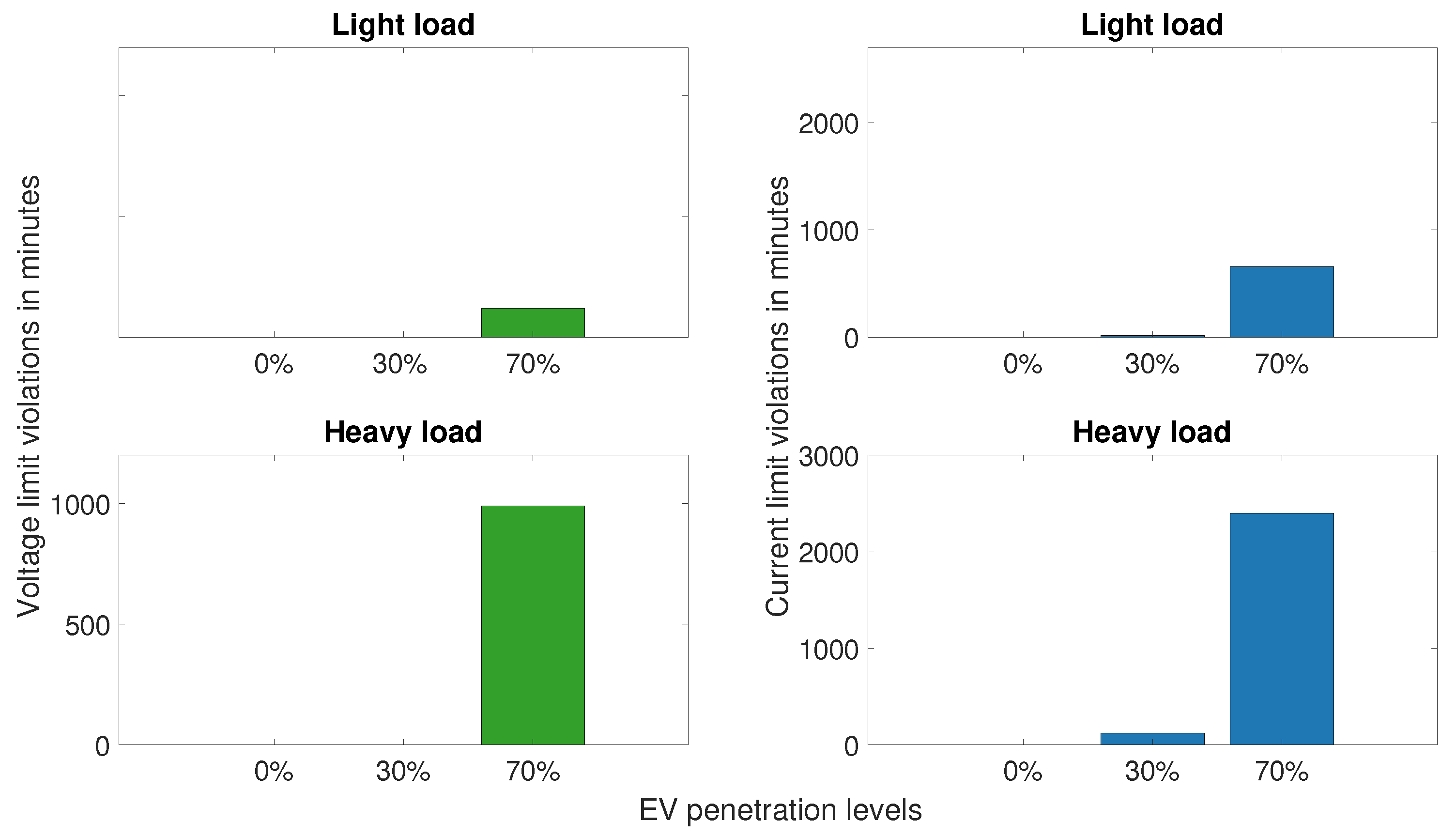
We firstly assess the impact of UC. As already mentioned, we define two baseload cases (light and heavy load) for the simulation. The two load cases were combined with three penetration scenarios to check which constellation has the greatest impact on the investigated low voltage grid. We depict the results in
Figure 3 as a comparison of voltage and current limit violations in minutes, for both light and heavy load cases. The light and heavy load case show no violations when no EVs are integrated. With an EV penetration rate of 30%, we found no voltage violations in both light and heavy load scenarios. The current carrying capacity of the cable is exceeded for 15, 120 min, respectively. As for the heavy load scenario with a 70% EV penetration rate, voltage violations occur for 990 min and current limit violations for 2400 min. This highlights the fact that the impact of EV charging highly depends on the baseload of the considered grid.
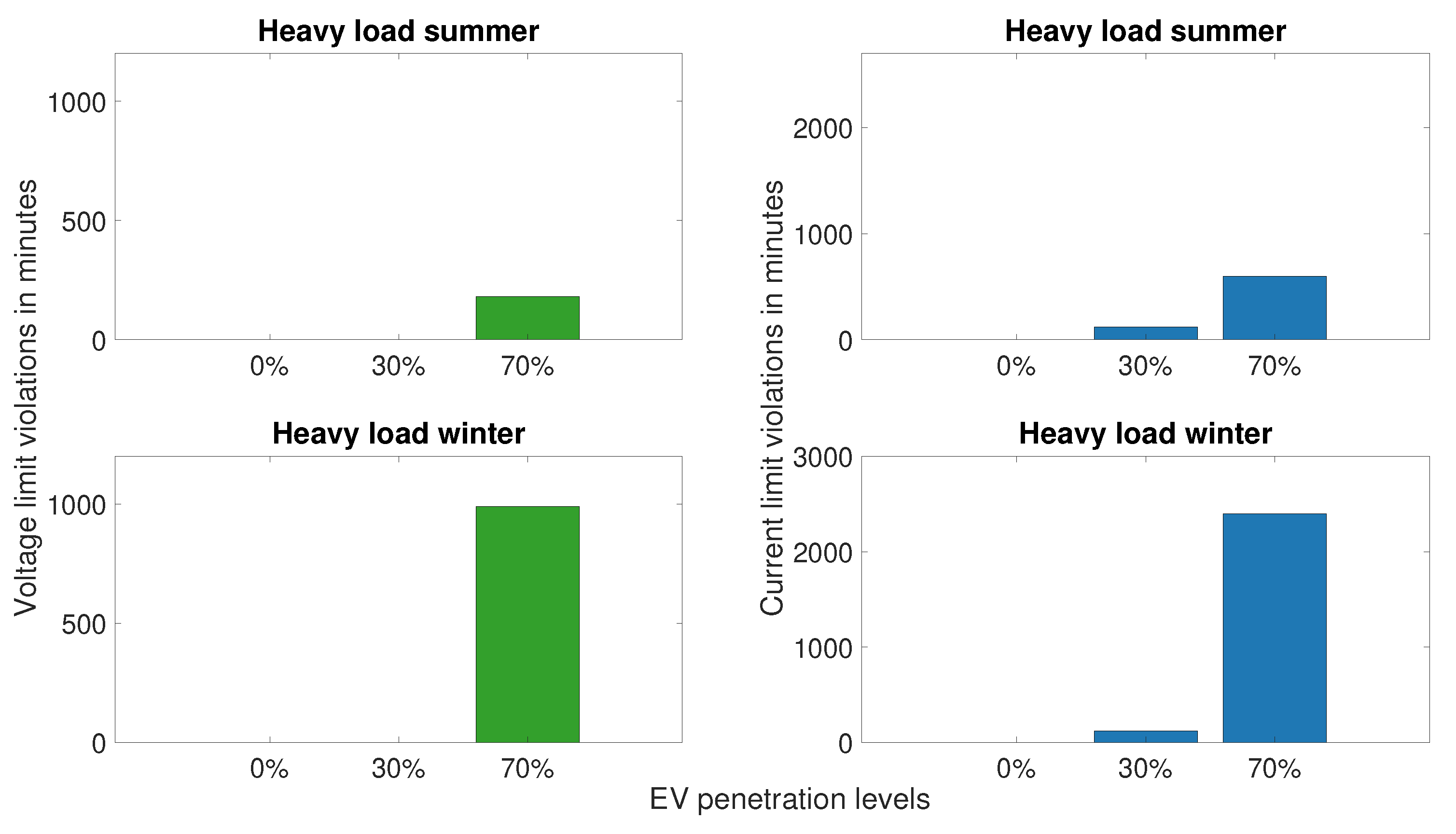
We also analyze the effects of the penetration scenarios for winter and summer to explore seasonal behavior. As the baseload is higher in winter than in summer and EVs have generally a higher energy consumption in colder month, the impact of EV charging is more pronounced in winter. The results are shown in
Figure 4. With a growing number of EVs, frequency and duration of violations increase and as the energy demand and baseload are higher in winter, more violations for both current and voltage limits occur during winter. The figures show that the most critical situations arise for the heavy load case in winter and summer with a 70% EV penetration rate (2050 scenario). This is why these constellations is our main focus for the application and impact studies of our optimization algorithms which can be found in
Section 4.2.
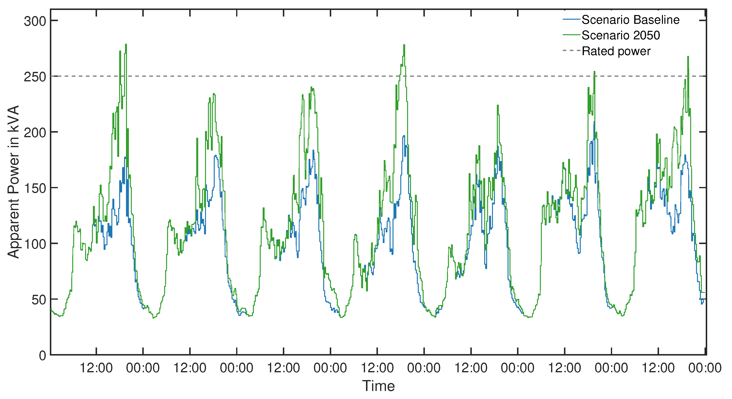
To elaborate on the reasons why we do not use the apparent power at the transformer and the rated power of said transformer as an analysis criterion, we use
Figure 5. It shows that even in a worst-case scenario (winter’s week, heavy load, and 70% EV penetration), the rated power limit is only exceeded for short periods and never reaches 130% of the rated power limit. Furthermore, we observe that the EVs are indeed adding to the evening peaks, and uncoordinated charging, considering our input data, rarely takes place during the night.
The key figures for UC are shown in
Table 2. The overall costs for one week are higher for the week in the summer because of general higher electricity prices in the selected summer week. Due to the higher electricity production from photovoltaic systems in summer, GHG emissions are around 70 kg CO
eq lower. Due to the higher baseload and EV charging demand, the network losses are higher in winter. We also checked electricity prices and GHG emissions for other weeks and received similar results. Therefore, we choose the depicted weeks for their representative character.
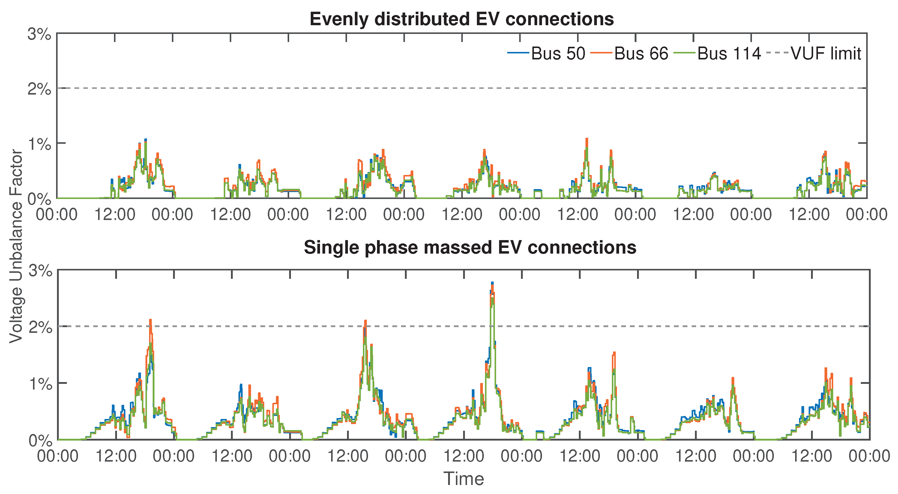
Practical experience has shown that single-phase installations tend to get connected to a specific phase. This was also confirmed with domain experts.
Figure 6 depicts a comparison of the voltage unbalances for two different cases at three different buses. For the first case, the phase connections are evenly distributed, whereas for the second case 70% of all single-phase installations are connected to phase R. Bus 66 is located near the transformer, Bus 50 in the middle, and Bus 114 at the end of the grid. In both cases, a balanced distribution of the households loads can be observed. In the night hours when no electricity is generated by photovoltaic systems, the voltage unbalance factor is 0%. In the case where the connections are evenly distributed among the phases, we can see that the voltage unbalance factor stays at about 1%. In the second case, the accumulation of connections to a single-phase leads to a violation of the limit for voltage unbalance. A peak value of 2.5% is reached. This shows that with an unfavorable phase distribution of EVs, the safe operation threshold for the grid is exceeded.
Another factor of impact is the distribution of EVs to the households in the grid. The further the EVs are connected from the transformer, the higher the voltage drops. Therefore, we analyze the distrubtion of EVs to the households and choose bus 114, which meets this criterion. As a single line connects the transformer to the rest of the grid, bus 1, was selected as benchmark. To study the worst-case scenario, all EVs were connected to households located as far as possible from the transformer, as well as 70% of all mono phase connections to the phase R.
Figure 7 shows a box plot for the phase voltages at bus 114 and currents at bus 1. The unsymmetrical loading of the grid is especially visible for the voltage values for phase R. The minimum values lie at 0.875 pu with a number of outliers between 0.875 and 0.85 pu. The phases S and T show almost the same voltage drop distribution. For phase R, 75% of all values lie above 0.945 pu, while for the phases S and T the figures are slightly higher than 0.95 pu. As for the current values, a massive violation occurs at phase R with maximum values up to 820 A, which is almost double the current carrying capacity of the cable. Similar to the voltages, the currents for phase S and T show a comparably light valuation with maximum values up to 580 A. More than 75% of the values for all phases lie beneath the current limit.
4.2. Coordinated Charging
In this section, the results for week-ahead scheduling are presented with regards to their respective saving potentials and impact on the electrical grid. The simulation was run over a week with 15-min time steps. If not stated otherwise, all results are based on the 2050 scenario for a winter week with heavy load and evenly distributed EVs, as well as PV installations.
4.2.1. Cost Optimized Strategy
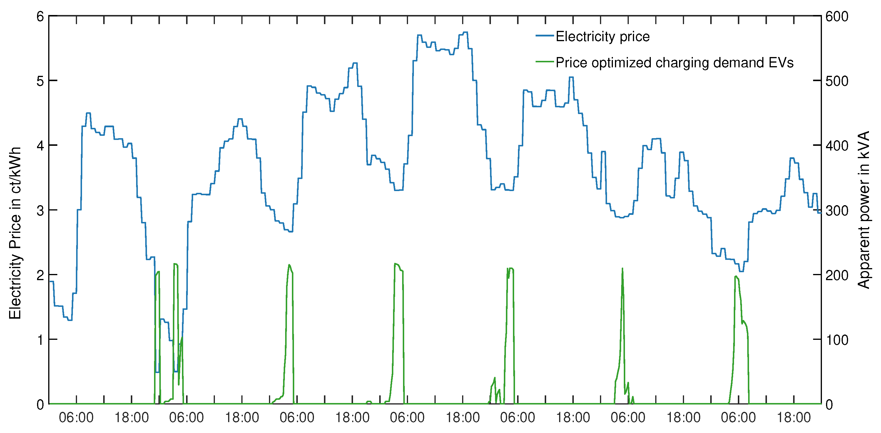
In
Figure 8, the results of the energy cost optimization are depicted for a week in winter. We see that the electricity wholesale prices are low during the night due to low demand. The charging events of the EVs are contained to a number of short time frames with the lowest electricity prices. Because of the transformer constraint, the charging demand of the EVs is limited to a peak of 167 kVA. In Equation (1d), we set the transformer limit LT to 200 kVA as in our specific network the current rating of the cable is exceeded before the apparent power rating of the transformer (250 kVA). A transformer limit of 200 kVA was chosen because it is the maximum apparent power value, at which the current does not exceed the given limit if the network is balanced.
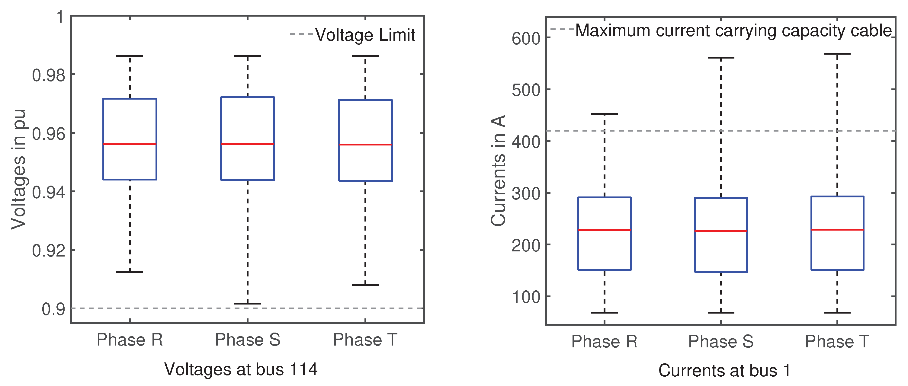
As shown in the right box plot of
Figure 9, this does not work as intended as EV charging is inherently unbalanced and the accumulation of EV charging on a single-phase leads to violation of the current-carrying limit, even when the apparent power limit is adhered. The medians of the phase currents lie at 226 A, and the whiskers are crossing the current-carrying limit. All boxes have the same height indicating that for all three phases, 50% of all values are distributed between 150 A and 290 A. The voltage limit is not exceeded with a median of 0.956 pu and the whiskers reaching from 0.986 pu to 0.902 pu.
The overall energy costs are
€ for the optimization with transformer constraint. The overall saving between UC and cost-optimized charging is
€ or 51.13%. Due to a high coincidence between low GHG emissions and low energy prices, the carbon emissions are almost halved, dropping from 924.54 to 548.89 kg CO
2eq. Network transmission losses are decreasing from 1.332 kVA to 0.895 kVA, due to the lower current peaks and the quadratic relation between current and losses. A summary of the changes in economic key figures and a comparison between the results for the different CC strategies can be also found in
Table 3.
4.2.2. VF Optimized Strategy
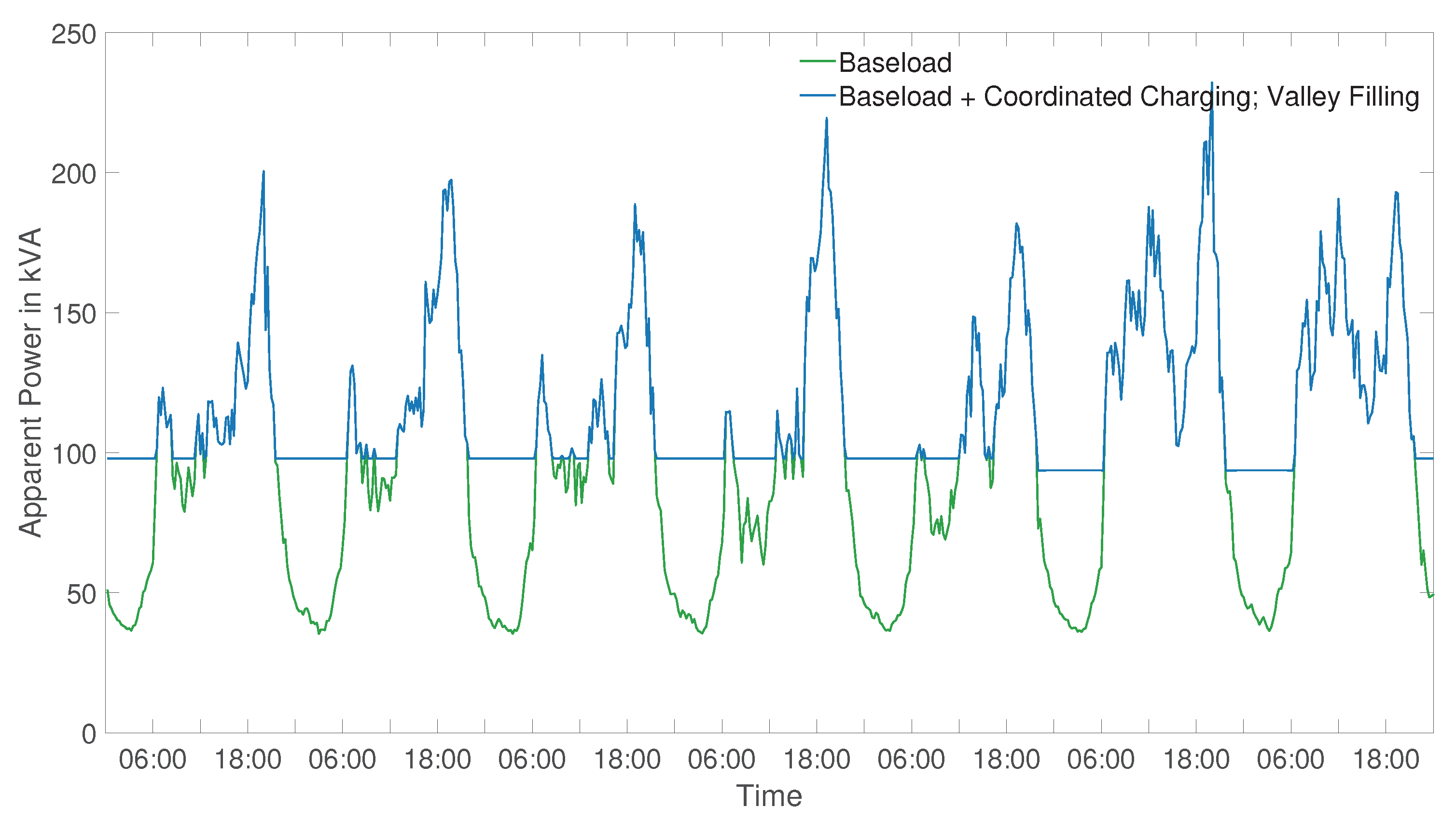
Figure 10 shows the graph of the apparent power in the base case without EVs compared to the VF CC approach. We can see that the valleys in the night are perfectly filled by the charging demands of the EV. Some EVs are charging forenoon so that the small load valley between breakfast and noon is filled, but the majority of EVs are charging between 8:00 p.m. and 8:00 a.m. the next day. Therefore, we can conclude that the parking times of the EVs are sufficient, to allow almost perfect scheduling.
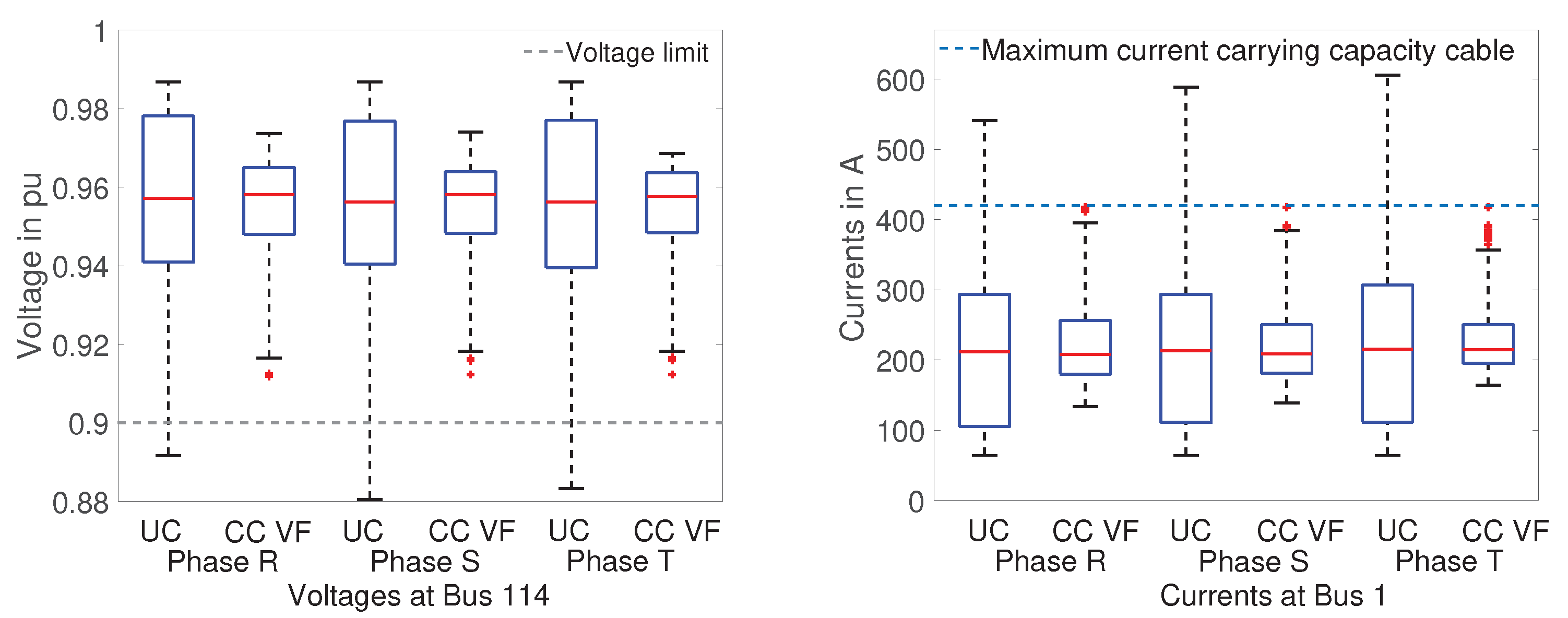
Figure 11 depicts box plots of the voltages and currents for each phase, at two critical buses in the network for the uncoordinated and the coordinated charging VF approach. For the VF approach, we can observe that in the heavy load case the currents at peak times are close to the current carrying capacity limit of the cable. The valley filling optimization allows the medians of the phase currents to drop slightly from around 211 A in the UC case to around 208 A in the CC case. Similar to the behavior of the phase voltages in the UC case, some current values violate the limits, and the distribution is wider, indicated by taller boxes and longer whiskers. The average network losses can be reduced from 1.332 kVA to 0.636 kVA, which makes this strategy the best overall strategy for the DSO. GHG emissions and electricity costs for EV charging are 890.85 kg CO
2eq and
€, respectively. SC is comparably low with 1.13% for the heavy load winter scenario, as the EVs are scheduled to charge predominantly at night.
4.2.3. GHG Emission Optimized Strategy
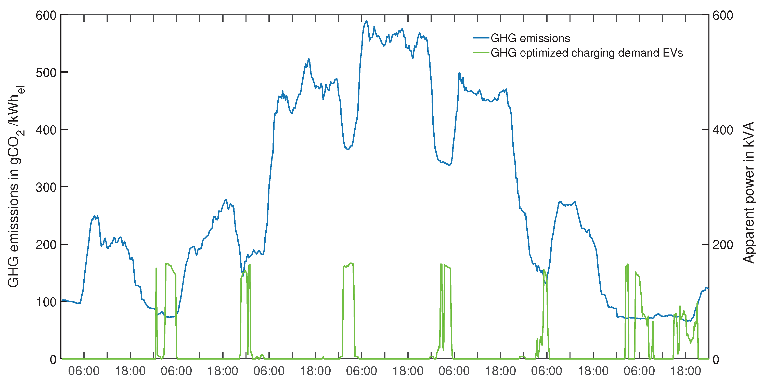
Environmental conscious EV users might want to charge their EVs with electricity that was generated by energy sources with a low carbon footprint. This optimization could be employed by load serving utilities to offer their customers a truly green energy tariff. The GHG-optimized charging demand is shown in
Figure 12. Due to a high feed-in of wind energy plants in the considered week in the winter, GHG emissions of the energy mix are low in the night. Additionally, EVs are generally available at home during this time and can be ideally scheduled. Overall GHG emissions drop from 924.54 kg CO
2eq in the case of uncoordinated charging (2050) to 517.50 kg CO
2eq when GHG-optimized charging is employed. The summed up electricity cost for the charging demand of the EVs lies at
€, which is comparably low due to the deployment of renewable energy sources. As the charging process is shifted into the night hours, a decrease in SC from 4.04% to 0.18% can be observed. Additionally, due to the shift into the night, the ADL drops to 1.105 kVA, which is caused by lower current flows in the network.
In
Figure 13, the distribution of phase voltages and currents is shown. The phase voltages are exhibiting nearly the same median value of around 0.96 pu, furthermore are the inter-quartile ranges almost equal. The whiskers span from 0.986 pu to 0.905 pu, indicating the minimal and maximal voltage drop. No violation in voltage limits occur. In contrast, the current carrying capacity of the cable is exceeded. The medians of the current values are nearly equal for all three phases at around 229 A. Moreover, 75% of all currents are below 300 A, but measurement 25% quantile reach a maximum of 469 A, 535 A, and
A, for phase R, S, and T, respectively. Therefore, the current carrying capacity of the cable is exceeded on multiple occasions, which could lead to an overheating of the cable.
4.3. Discussion of the Results
In
Table 3, a summary of the results for the economic key figures of the considered week in the winter (Scenario 2050) is given. The different optimizations are able to achieve their objectives. The cost optimization lowers the energy cost by more than half and provides the user with the lowest overall energy cost among the other optimizations. Due to the relation between the employment of low carbon technologies and low energy prices, it significantly lowers GHG emissions. The GHG-optimized charging offers only a 5.6% reduction of emissions, at a cost increase of 26.29% in contrast to the cost optimized scenario. This is due to low carbon emission technologies being deployed during a time of high demand and therefore, high electricity prices. This fact can also be observed when the ADL are compared. The cost-optimized charging offers a reduction of 30%, while GHG optimization only offers a 17% reduction in comparison to the UC scenario. As network losses are mainly a quadratic function of current, this underlines the fact, that EVs were scheduled to charge during a time of high load. These circumstances make GHG minimal charging economically infeasible, at least in the week that was studied here. The SC is low for both optimizations as the EV are mainly charged at night, and SC levels are in general low in winter. VF provides the lowest ADL but results in comparatively high energy costs and GHG emissions. As VF is most suitable from a grid perspective and thus a potential strategy for DSOs, our results emphasize the conflict of interest that could occur between operators and aggregators.
5. Outlook and Future Work
In this paper, we developed a simulation model for a European semi-urban low voltage grid. We designed the grid model in MATLAB Simulink and implemented an algorithm for the automatic generation of the grid model. Our model provides the option to modify many input parameters very easily, e.g., the penetration of PV installations or the number of EVs. The resulting output parameters are comprehensive and include among others voltages and currents per phase. Using the model, we analyzed the impact of uncoordinated charging on different output parameters. Subsequently, we developed three different optimization-based coordinated charging strategies. The main impacts we assessed include voltage drops, phase unbalances and electrical grid losses. The interactions of the EV charging processes and a representative distribution grid, presented in this paper, demonstrate the importance of an EV impact study.
For our semi-urban low voltage grid, an EV penetration rate of 30% shows almost no noticeable impact. However, when we take a look in the year 2050 with an EV penetration rate of 70% and a PV penetration rate of 33%, we see some interesting results. No violations of the additional criterion of voltage unbalance can be observed if the fleet is evenly distributed among the phases. Nevertheless, in real-world systems it is impossible to control at which phase an EV will be connected to. Our further analysis of a non evenly distributed fleet among phases showed an excess of the voltage unbalance limit.
The VF approach proved to be the best way to minimize network losses but has the disadvantage of comparably high GHG emissions and electricity costs. The cost optimized strategy is able to minimize the costs for electricity but leads to critical grid situations even with a constraint on the apparent power flow in place. The GHG emissions optimized strategy helps to reduce GHG emissions by around 40%. In contrast to VF, the average electrical distribution losses increase by around 30%.
The above analysis and results include a representative topology and realistic methodology to measure the EV impact on low voltage grids. From the results, it is observed that there are conflicts between different approaches. Decision makers should trade-off the different objectives and outcomes, alleviating electricity costs, grid congestion, and GHG emissions. Regardless of the policy followed, we conclude that analyzing the impact of EVs, particularly as EV battery sizes are increasing, is of paramount importance. This study provides a practical and representative basis for future analysis.
With the grid model created in this work, further research into more advanced optimization algorithms is possible. One future research direction could be the implementation of an algorithm which is directly coupled to the electrical grid model. In this case, more realistic scheduling of EV could be reached by taking shorter optimization horizon into account.


